Study on the large scale dynamo transition

Abstract

Using the magnetohydrodynamic (MHD) description, we develop a nonlinear dynamo model that couples the evolution of the large scale magnetic field with turbulent dynamics of the plasma at small scale by electromotive force (e.m.f.). The nonlinear behavior of the plasma at small scale is described by using a MHD shell model for velocity field and magnetic field fluctuations.The shell model allow to study this problem in a large parameter regime which characterizes the dynamo phenomenon in many natural systems and which is beyond the power of supercomputers at today. Under specific conditions of the plasma turbulent state, the field fluctuations at small scales are able to trigger the dynamo instability. We study this transition considering the stability curve which shows a strong decrease in the critical magnetic Reynolds number for increasing inverse magnetic Prandlt number $\textrm{Pm}^{-1}$ in the range $[10^{-6},1]$ and slows an increase in the range $[1,10^{8}]$. We also obtain hysteretic behavior across the dynamo boundary reveling the subcritical nature of this transition. The system, undergoing this transition, can reach different dynamo regimes, depending on Reynolds numbers of the plasma flow. This shows the critical role that the turbulence plays in the dynamo phenomenon. In particular the model is able to reproduce the dynamical situation in which the large-scale magnetic field jumps between two states which represent the opposite polarities of the magnetic field, reproducing the magnetic reversals as observed in geomagnetic dynamo and in the VKS experiments.

One of the most fascinating and challenging topics in physics and astrophysics is the understanding of the generation and self-sustaining of magnetic fields in planets, stars, galaxies, etc. The most accredited mechanism is the so-called dynamo effect, i.e. the maintaining of a magnetic field against diffusive effects by the motion of electrically conducting fluids. This effect has also been studied in laboratory liquid metal experiments like Riga and VKS experiment experiment and plays a fundamental role in our understanding of many magnetized phenomena which are of interest in many research fields since Faraday’s study.

The dynamo effect occurs because magnetic field lines are generally stretched at small scales by the random motion of the fluid in which they are almost ‘frozen’. The magnetic lines stretching leads to an exponential amplification of the field, until the backreaction (via the Lorentz force) causes the saturation of this growth. The small–scale dynamo is generated when the system reaches energy equipartition at small scales. During the growth of the magnetic energy at small scales, the velocity and magnetic field fluctuations interacts each other, generating an e.m.f. able to produce a large scale magnetic field. The latter increases due to the turbulent fluctuations at small scales until a saturation level is reached. The dynamo quenching occurs because the system attempts to conserve the total magnetic helicity when the magnetic field is growing Brandenburg (2009).

In the present Letter we investigate the dynamo effect driven solely by turbulent fluctuations, in absence of a mean flow ($\alpha^{2}$–dynamo), focusing our study on the dynamical transition towards the regime where the large scale magnetic field starts to be generated. Dynamo transition results from an instability: when, for an assigned value of the Reynolds number $Re\simeq\delta u/k_{0}\nu$, the magnetic Reynolds number $\textrm{Rm}\simeq\delta u/k_{0}\mu$ ($\delta u$ being the r.m.s. of the turbulent velocity, $\nu$ and $\mu$ respectively the kinetic viscosity and the magnetic diffusivity) reaches a critical value $\textrm{Rm}_{c}$, the magnetic field looses its stability from a quasi zero–magnetic field state generating the initial exponential increasing in its values until the dynamo quenches. Generally, the dynamo bifurcation could display at least two different natures: subcritical and supercritical sub-super-critical , in analogy with turbulent transitions. We want to investigate its nature, using a new model, recently built up, with the aim to overcome the limitation in the Reynolds number range covered by both direct numerical simulation (DNS) and by a lot of other theoretical models. In fact, although DNS are playing an important role in our understanding of the dynamo problem (Kagemayama et al., 2008), a realistic parameter regime is still beyond the power of supercomputers at today. Difficulties arise from the very large values of the dimensionless parameters, which characterize this problem in natural systems.

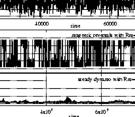
Figure 1: Time evolution of the large scale magnetic field in dimensionless units in different simulations. The system starting from oscillatory behavior, undergoes the transition to reversals regime and finally reaches a steady dynamo for increasing values of the Reynolds numbers.

In 1955, Parker Parker (1955) suggested that the net effect of averaging many small scale turbulent motions would be to produce the large scale electric field ($\alpha$ effect) generating large scale poloidal and toroidal magnetic field. The latter can also be generated by the differential rotation ($\alpha$-$\Omega$ effect). In the same spirit (see also Perrone (2010)), we make a decomposition of the fields in an average part, varying only on the large scale $L$, and a turbulent fluctuating part, varying at small-scales $\sim\ell$, with the assumption $\ell\ll L$ (Biskamp, 1993). Performing this scale separation we obtain, in the induction equation at large scale, a term which describes the action of small scales on the large one consisting in a turbulent e.m.f. that can be written in terms of the Fourier modes of velocity (${\bf{u}}({\bf{k}},t)$) and magnetic field (${\bf{b}}({\bf{k}},t)$) small scale fluctuations as follow:

$${\bf{\epsilon}}=-\sum_{\bf{k}}{\bf{u}}({\bf{k}},t)\times{\bf{b}}^{*}({\bf{k}},t)\ ;$$ (1)

this is a correlation between velocity and magnetic field fluctuations at small scales. Introducing a basis in the spectral space: $\ \ \widehat{e_{1}}({\bf{k}})\ ,\ \ \widehat{e_{2}}({\bf{k}})=\widehat{e_{3}}({\bf{k}})\times\widehat{e_{1}}({\bf{k}})\ ,\ \ \widehat{e_{3}}({\bf{k}})=i{\bf{k}}/|{\bf{k}}|$; and writing expression (1) in a form symmetric with respect to the change of ${\bf{k}}$ in $-{\bf{k}}$ we finally find:

$${\bf{\epsilon}}=-\sum_{\bf k(k_{z}>0)}\widehat{e_{3}}\ [(u_{1}^{*}\ b_{2}-u_{2}\ b_{1}^{*})+(u_{2}^{*}\ b_{1}-u_{1}\ b_{2}^{*})]$$ (2)

where $u_{1}$ and $u_{2}$ ($b_{1}$ and $b_{2}$) are the components of ${\bf{u}}({\bf{k}},t)$ (${\bf{b}}({\bf{k}},t)$), along $\widehat{e_{1}}$ and $\widehat{e_{2}}$.

We describe the dynamics of the system at large scale by integrating the induction equation in local approximation: we approximate the toroidal ($\widehat{e_{\varphi}}$) and the poloidal ($\widehat{e_{p}}$) unit vectors with the cartesian unit vectors, respectively $\widehat{e_{x}}$ and $\widehat{e_{z}}$. Hence the field at large scale are:

$${\bf{u}}_{0}=V(y,z)\ \widehat{e_{x}}\;\;,\;\;\;\;{\bf{b}}_{0}=B_{\phi}(y,t)\widehat{e_{x}}+B_{p}(y,t)\widehat{e_{z}}$$ (3)

where ${B}_{\phi}$ and ${B}_{p}$ are the toroidal and poloidal component of the magnetic field, respectively. We describe the dynamics at small scales by a shell model Frick and Sokoloff (1998), where the wave vectors space, in which one considers the MHD equations, is divided into a finite number N of shells of radius $k_{n}=2^{n}k_{0}$ (with n= 0,1,…,N; and $k_{0}\sim 2\pi/\ell$ is the fundamental wave vector). In each shell is assigned complex scalar variables $u_{n}(t)$ and $b_{n}(t)$, describing the dynamics of velocity and magnetic Fourier modes in the shell of wave vectors between $k_{n}$ and $k_{n+1}$. The nonlinear coupling of neighbor shells is chosen by preserving total energy, cross helicity, and magnetic helicity, and, at variance with the original MHD shell model, avoiding unphysical correlations of phases. We can write the set of self-consistent equations for our dynamo model in which the e.m.f. is in a form consistent with the shell model:

$$\frac{d{B}_{\phi}}{dt}=\frac{i}{L}\sum_{n}({u}_{n}^{*}{b}_{n}-{u}_{n}{b}_{n}^{*})+{B_{p}\frac{V}{L}}-\mu\frac{{B}_{\phi}}{L^{2}}\ ,$$ (4a)

$$\frac{d{B}_{p}}{dt}=\frac{i}{L}\sum_{n}({u}_{n}^{*}{b}_{n}-{u}_{n}{b}_{n}^{*})-\mu\frac{{B}_{p}}{L^{2}}\ ,$$ (4b)

$${\frac{d{u_{n}}}{dt}}=k_{n}({B}_{\phi}+{B}_{p})b_{n}+{\rm i}k_{n}\Big{[}(u_{n+1}^{*}u_{n+2}-b_{n+1}^{*}b_{n+2})+$$

$$-\frac{1}{4}(u_{n-1}^{*}u_{n+1}-b_{n-1}^{*}b_{n+1})+\frac{1}{8}(u_{n-2}u_{n-1}-b_{n-2}b_{n-1})\Big{]}$$

$$\;\;\;\;\;\;\;\;\;\;\;\;\;\;\;-\nu k_{n}^{2}u_{n}+f_{n},$$ (4c)

$${\frac{d{b_{n}}}{dt}}=ik_{n}({B}_{\phi}+{B}_{p})u_{n}+\frac{ik_{n}}{6}\Big{[}(u_{n+1}^{*}b_{n+2}-b_{n+1}^{*}u_{n+2})$$

$$+(u_{n-1}^{*}b_{n+1}-b_{n-1}^{*}u_{n+1})-(u_{n-2}b_{n-1}-b_{n-2}u_{n-1})\Big{]}$$

$$\;\;\;\;\;\;\;\;\;\;\;\;\;\;\;-\mu k_{n}^{2}b_{n};$$ (4d)

where the spatial derivative associated at large scale is estimated dividing by the typical large scale L; $\nu$ is the viscosity and $\mu$ is the diffusivity of the MHD flow; $n$ is the shell number ($n=0,...N$); finally $f_{n}$ is an external forcing term applied on the first shell ($n=0$). This forcing, that drives the fluid flow to become unstable, has the property to preserve the energy flux to small scales. This is the same forcing used in Nigro & Carbone (2010) with correlation time equal to 1. The first terms in the RHS of Eqs. (4c)-(4d) describe the effect of the large scale magnetic field on the small–scale turbulent dynamics. Due to these terms, the turbulence becomes anisotropic because the field fluctuations self organize themselves in coherent structures, channeled along the large scale magnetic field $\bf b_{0}$ as Alfvén waves.

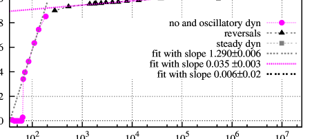
Figure 2: (Color online) Dynamical behavior of $\delta b/\delta u$ for increasing Rm. Starting from no magnetic field state, we check the values of $\delta b/\delta u$ during the running time of the simulation in which we increase Rm for $\nu=10^{-5}$. During this time the system undergoes dynamo transition (magenta circles) reaching oscillatory regime, afterwards the system goes towards reversals regime (black triangles) coming to steady states where the large scale magnetic field saturates (gray squares).

We have obtain the e.m.f. consistently with shell model without linear approximation. The e.m.f. tends to vanish when the system evolves towards a state of strong correlation between velocity and magnetic field, which characterizes the Alfvénic subspaces. This is an attractor of the dynamics of the system dobrowolny80 . We solve the model Eqs. assuming $V=0$, that is equivalent to solve the dynamo problem for Rossby number $\textrm{Ro}=\frac{\delta u}{V}\frac{\delta b}{B_{p}}\gg 1$. Hence ${B}_{p}(t)={B}_{\phi}(t)=\textrm{B}(t)$ and the model describes $\alpha^{2}$ dynamo problem, in which the shear due to the differential rotation at large scale is neglected. Even in the absence of the macroscopic shear, the $\alpha$ effect can give rise to dynamo action. This effect seems to play a decisive role for planetary magnetic fields as geomagnetic field. It can be very strong in the fully convective stars as the late-type stars and it may provide a possible mechanism to explain magnetic activity, along with nonaxisymmetric field as observed in many active stars Meinel & Brandenburg (1990).

The model Eqs. are numerically solved by using a fourth order Runge-Kutta scheme. The results are in dimensionless units: the field fluctuations are measured in Alfvén velocity unit $c_{A}$, the time in eddy-turn-over time ($1/(k_{0}u_{0})$), the lengths are normalized to $1/k_{0}$, and finally the dissipative coefficients are normalized to $c_{A}/k_{0}$.

At the beginning of each simulation, we let the system become turbulent at small scales, i.e. we keep $\textrm{B}=0$ up to $1000$ unit times. During this time the kinetic and the magnetic energy at small scales grow forming a power law spectrum. The system tends to the energy equipartition at small scales, exactly achieved when $\nu=\mu$. After that, when we are sure that the turbulence is fully developed, we introduce a magnetic field seed of amplitude $10^{-10}$ at large scale and we check whether the dynamo effect starts to develop.

Figure 3: The stability curve $\textrm{Rm}_{c}$ vs $\textrm{Pm}^{-1}$ in log scale. The inset in semi–log scale shows the slight increase of $\textrm{Rm}_{c}$ for increasing $\textrm{Pm}^{-1}>1$.

The numerical results reveal a strong sensitivity of the system with respect to the magnetic Reynolds number Rm and a dependence on the hydrodynamic Reynolds number Re. Depending on these parameters, the system evolves towards different scenarios: i) no dynamo; ii) oscillatory dynamo; iii) magnetic reversals; iv) steady dynamo. The transition from oscillatory dynamo to a steady dynamo, going through a reversals regime, is obtained by increasing Re and Rm (Fig. 1), reproducing in this way the same dynamo regimes as observed in the liquid metal experiments experiment .

In order to better characterize the different regimes, we have performed a simulation with a fixed value of the kinematic viscosity but changing the value of the magnetic diffusivity after a time interval sufficiently long with respect to the dynamical evolution times and we have studied how the two parameters $\delta b/\delta u$ and $rms(\textrm{B})/\delta u$ change with the magnetic Reynolds number Rm.

The $\delta u/\delta b$ function illustrated in Fig. 2 for increasing Rm shows a zero order discontinuity corresponding to dynamo transition (the step for $\textrm{Rm}=67$) and a first order discontinuity corresponding to the transition from oscillatory dynamo to reversals regime. The kind of these discontinuities marks the different nature of the transitions, in particular we can argue that the dynamo effect occurs as a plasma instability while the others transitions occur with continuity.

Our model allows us to study the dynamo instability inside a very large values of critical parameters not accessible by DNS yet, but more realistic for the astrophysical objects. We have investigated the dynamo threshold for different Prandlt number, reproducing the stability curve in a very wide range of values, illustrated in Fig. 3, which shows a little dependence of $\textrm{Rm}_{c}$ for $\textrm{Pm}^{-1}>1$; and a strong monotonic increase of $\textrm{Rm}_{c}$ for decreasing $\textrm{Pm}^{-1}<1$. The reason of this strong increase could be related to the need to have small magnetic diffusivity to compensate the large viscosity in order to have small scales field fluctuations large enough, to consistently trigger the e.m.f. at large scale for the dynamo onset. On one hand, this result is consistent with what was obtained by other models in a smaller range of critical parameters: $\textrm{Pm}^{-1}\in[1,100])$ stability-curve , giving us the possibility to be confident on our model, and on the other hand, it extends these results in larger range of values not investigated yet. The model hence reaches values more realistic for the astrophysical objects. For instance, for interstellar or intracluster medium $\textrm{Pm}\gg 1$, in the Sun’s convective zone, $\textrm{Pm}\sim 10^{-7}$ to $\sim 10^{-4}$, in planets $\textrm{Pm}\sim 10^{-5}$ and in protostellar disks $\textrm{Pm}\ll 1$.

The dynamo onset could take place in subcritical or supercritical way. In some models and experiments it is subcritical, as it has showed in some small–scale dynamos, revealing a hysteretic behavior hysteresis .

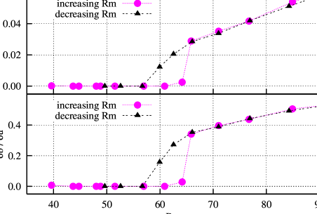
Figure 4: (Color online) Hysteresis cycles of $\textrm{rms}(\textrm{B})/\delta u$ (top panel) and $\delta b/\delta u$ (bottom panel) obtained around the stability margin of the bifurcation for the simulation with $\nu=10^{-5}$ and changing Rm: we increase Rm reaching dynamo onset in which the magnetic field displays oscillations (first phase: magenta circles), afterwards we decrease Rm (second phase: black triangles).

In order to investigate the nature of this instability as described in our model, we have reproduced hysteresis cycles realized as following: for a fixed value of $\nu$, starting from a state of quasi zero–magnetic field characterized by low Rm, we have dynamically increased Rm during the simulation time in order to destabilize the system from the initial state. During the simulation we have checked the time evolution of the order parameters: the ratio between the r.m.s. of B over $\delta u$ and $\delta b$ over $\delta u$. Only after a critical value of Rm, corresponding to the threshold for the dynamo action to set up, we have found the increase of the large scale magnetic field (first phase). Once the dynamo sets in, we have decreased Rm (second phase). In the second phase, order parameters not follow the path inverse to the first phase, realizing a hysteresis loop. We have investigated hysteresis cycles considering a wide range of values of $\nu$ down to $10^{-11}$. For the example reported in Fig. 4 where $\nu=10^{-5}$, starting from a quasi null magnetic field, we have increased Rm up to $\textrm{Rm}_{c}=67$, corresponding to the dynamo threshold, by finding for the order parameter the values shown by the magenta circles in Fig. 4. After the dynamo onset, keep increasing Rm, the system displays magnetic oscillation and subsequently magnetic reversals. Once reached these regimes, we have decreased Rm. The values of the order parameters, representing now by the black triangles, lie on the same curve when the system is in latter regimes, afterwards the order parameters lie on a different curve starting from $\textrm{Rm}_{c}$ to lower values. This shows the hysteretical behavior of the transition and its subcritical nature. We have found also a slight suppression of hydrodynamic turbulence during the transition Cattaneo et al (1996), revealed by the decrease of hydrodynamic Reynolds number $\textrm{Re}\simeq\delta u/k_{0}\nu$. In the example in Fig. 4, Re, starting from a value around $8000$, slightly decreases to $7000$ when the dynamo action is developed. We can argue that the subcritical nature of dynamo bifurcation could come out from the reduction of turbulence due to the magnetic field growing, which ensure the maintain of the dynamo effect for lower Rm values.

We present a dynamo model developed for the large scale magnetic field. The model solves the induction equation in local approximation at large scale, while the turbulent dynamics at small scales is described by a MHD shell model. We point out that there is no prescribed form (like $\alpha$-term) for e.m.f., but it is consistently described by the analytical form of the shell model. Moreover at variance with others dynamo shell models Nigro & Carbone (2010); Benzi & Pinton (2010) which use ad hoc terms to mimic the dynamo instability, this model is able to reproduce different regimes in dynamical way without any ad hoc assumption. An important result of this research is related to the critical role that the turbulence plays in the dynamo phenomenon showing how different regimes are obtained depending on Reynolds numbers of the plasma flow. This property of the model is also confirmed by laboratory experiments inside the Reynolds number accessible to these. One of the strength of our model, due to the use of the shell technique, consists of the capability to describe the dynamo transition and the different regimes where it can act in a very large values of the Reynolds numbers. The study on the dynamo transition shows its subcricital nature supported by hysteresis cycles around the stability margin of the bifurcation. The model reproduces results consistent with other dynamo models in the parameter range accessible to these, therefore showing its reliability. Moreover it makes a step forward in our understanding of the dynamo problem due to its capability to cover a larger range of values not yet accessible by others models and by DNS, but more realistic for a natural dynamo processes. Finally we consider the results here obtained a good stimulus for both DNS and experimental studies on this problem.

References

- (1) A. Gailitis et al., Phys. Rev. Lett. 84, 4365 (2000); A. Gailitis et al., Phys. Rev. Lett. 86, 3024 (2001); R. Monchaux et al., Phys. Rev. Lett. 98, 044502 (2007); F. Ravelet et al., Phys. Rev. Lett. 101, 074502 (2008).
- Brandenburg (2009) A. Brandenburg, Plasma Phys. Control. Fusion 51, 124043 (2009).
- (3) P. Manneville, Dissipative Structures and Weak Turbulence (Academic Press, Boston, 1990); V. Morin, E. Dormy, International Journal of Modern Phys. B, 23, 5467 (2009).
- Kagemayama et al. (2008) A. Kageyama, T. Miyagoshi and T. Sato, Nature letters 454 1106 (2008); J. Li, T. Sato and A. Kageyama, Science reports 295 1887 (2002).
- Parker (1955) E. N. Parker, Astrophys. J. 122, 293-314 (1955).
- Perrone (2010) D. Perrone, G. Nigro and P. Veltri submitted (2010).
- Biskamp (1993) D. Biskamp, Nonlinear Magnetohydrodynamics, Cambridge University Press (1993).
- Frick and Sokoloff (1998) P. Frick and D. Sokoloff, Phys. Rev. E 57 4155 (1998); P. Giuliani and V. Carbone, Europhys. Lett. 43 527 (1998).
- Nigro & Carbone (2010) G. Nigro and V. Carbone, Phys. Rev. E 82 016313 (2010).
- (10) M. Dobrowolny, A. Mangeney, and P. Veltri, Phys. Rev. Lett. 45, 144 (1980).
- Meinel & Brandenburg (1990) R. Meinel and A. Brandenburg, Astron. Astrophys., 238, 369 (1990).
- (12) A.A. Schekochihin et al., Astrophys. J. 625 L115 (2005); A. Brandenburg, Astrophys. J. 550 824 (2001); Y. Ponty et al., Phys. Rev. Lett. 94 164502 (2005); A. Brandenburg, Astrophys. J. 697 1206 (2009).
- (13) G. Sahoo, D. Mitra, R. Pandit, Phys. Rev. E 81 036317 (2010); Y. Ponty et al., Phys. Rev. Lett. 99 224501(2007).
- Cattaneo et al (1996) F. Cattaneo et al., Phys. Rev. Lett. 76 2057(1996).
- Benzi & Pinton (2010) R. Benzi and P.J. Pinton, Phys. Rev. Letters 105 024501(2010).