An optical model for an analogy of Parrondo game and designing Brownian ratchets

Abstract

An optical model of classical photons propagating through array of many beam splitters is developed to give a physical analogy of Parrondo’s game and Parrondo-Harmer-Abbott game. We showed both the two games are reasonable game without so-called game paradox and they are essentially the same. We designed the games with long-term memory on loop lattice and history-entangled game. The strong correlation between nearest two rounds of game can make the combination of two losing game win, lose or oscillate between win and loss. The periodic potential in Brownian ratchet is analogous to a long chain of beam splitters. The coupling between two neighboring potential wells is equivalent to two coupled beam splitters. This correspondence may help us to understand the anomalous motion of exceptional Brownian particles moving in the opposite direction to the majority. We designed the capital wave for a game by introducing correlations into independent capitals instead of sub-games. Playing entangled quantum states in many coupled classical games obey the same rules for manipulating quantum states in many body physics.

I Introduction

It is an old saying from Chinese philosophers 3,000 B.C. that when a thing approaches to its extreme point step by step, it will finally transform into the opposite thingiching . Scientific discoveries stem from different fields to expand this philosophical idea. In engineering mechanics, combing two unstable system in the correct way may produce a stable systemallison . Parrondo devised a game to show the combination of two losing games may lead to an ultimate wining gameparrondo1996 . This game paradox was used to explain the directional motion of molecule motors by combining two random Brownian motion according to Parrondo’s game paradoxharmer . In quantum frustrated spin system, quantum fluctuation or thermal fluctuation which is supposed to destroy ordering results in long-range magnetic orderingchubukov , this is termed as order from disordervillian .

At first sight, Parrondo’s game is counterintuitive. Suppose a player has capital $100$ in beginning. He plays two losing game: game A and game B. If he only plays game A, the capital will drop. If he only plays game B, the capital drops too. If he plays game A many times, the capital drops, he switch to play game B many times, the capital continuous to drop, and then he switch to play game A again, and so on. One would intuitively expect that the player will finally lose, if the player wins instead, the game may be called a paradox. In fact, if there is no any correlation between the nearest two rounds of game, no matter how the player switch between two losing games, the final game will lose, it is indeed a paradox if the game wins instead. But if there exist correlation between the nearest two rounds of losing games or any two rounds of game, the combination of two losing games could be a win, a loss or oscillation between win and loss. It depends how the correlation is planted among different games.

Parrondo’s game introduced the correlation between the nearest two rounds of game. Parrondo, Harmer and Abbott proposed a history-dependent game paradoxparrondo as an improvement of Parrondo’s gameparrondo1996 . Later on, the history-dependent game paradox was extended to couple two history-dependent gameskay . The history-dependent game paradoxparrondo consists of two games: game A and game B. The game A is a biased coin which has probability $p$ to win and probability $1-p$ to lose. The players of game B are four coins whose strategy at each step depends on previous two steps in historyparrondo . Both Parrondo’s game and this history dependent game are mathematical issue which study the relationship between the winning or losing probabilities of two coupled games.

An indivisible classical photon scattered by a beam splitter is a perfect analogy of coin. If one plays a coin 100 times, it faces up 80 times and faces down 20 times, we say the winning probability is $0.8$, and losing probability is $0.2$. Each time the coin faces up, the point increase by $+1$, on the contrary, we has $-1$ point upon input capital. The final gain of this game is $(+80-20=+60)$. Therefore this is winning game. We let a photon collide with the beam splitter 100 times, it passed the beam splitter 80 times and is reflected by the beam splitter for 20 times. The reflection coefficient is $0.2$ and the transmission coefficient is $0.8$. Photon is electromagnetic wave. As we know, there is a $e^{i\pi}$ phase shift whenever a wave is reflected. Thus the reflected photon naturally carries a negative sign $e^{i\pi}=-1$. When two waves meet each other with $\pi$ phase difference, the destructive interference reduce the overlapping intensity to zero. In the language of photon, negative photon will annihilate with positive photon. If we let 100 uncorrelated photons collide with the beam splitter, and put the reflected photon and transmitted photon together, the number of survived photons is $(+80-20=+60)$. The classical photon is not only analogy of a coin, but also a solid physical implementation.

I will use photons passing through beam splitter array to give an almost exact implementation of both Parrondo’s game and the history-dependent game. The difference is Parrondo-Harmer-Abbott game does not have the negative sign $-1$ for the lost coins in their mapping matrix. While I will keep the $e^{i\pi}$ phase shift for every reflected photon. There are other ways to realize similar probability relation, such as special dices, quantum particles passing two slits, an so on. A light beam propagating through a network of mirrors(or more accurately beam splitters) is a very familiar phenomena for most people. This optical system give us a clear picture to show how the probability flow transform from loss to win, and vice verse.

Playing game will produce a time series recording the instantaneous value of output capital. We map every time series into an unique path in spatial degree of freedom. One can combine many losing or winning games by drawing optical diagrams. A real optical system provide a practical way to test those complex graphical design. Parrondo’s game only combines two games. What I demonstrated in this optical model is a diagrammatic method to combine many games(the number is at least larger than three). Every local game may be a loss or win. When many of these games are connected to form a complex network, one has to calculate to see the final output. The correlation between neighboring games play the key role in determining the final output.

The coupling between two neighboring beam splitters provide a direct understanding to the directional motion of Brownian particles in periodic asymmetric potential. The combination of the two losing games in Parrondo’s game paradox was used to explain Brownian ratchetharmer . In fact, what really matters is the strong coupling between neighboring potential wells. Every local potential well behaves like single beam splitter. The backward probability is turned into forward probability through two continuous steps of reflection by two neighboring potential wells. The optical model suggest that Brownian particle in periodic asymmetric potential does not always move in one designed direction, they can oscillate back and forth, or move in the opposite direction to the designed one.

The article is organized as follows:

In section II, we take a classical photon traveling across the array of beam splitters as analogy of Parrondo-Harmer-Abbott game. A different transfer matrix from that of Parrondo-Harmer-Abbott game is derived by considering the phase shift of reflection beams. When both sub-games lost, the final output of this optical game could be a win, a lose or oscillating between a win and a loss.

In section III, Parrondo game is also expressed into my optical analogy. The modular operation in Parrondo game is equivalent to a special beam splitter. The optical diagram has the same structure as that of Parrondo-Harmer-Abbott game.

In section IV, we designed the fractal history tree of a generalized history dependent game with longer memory, and extend it to the loop lattice of many beam splitters. We calculated the numerical eigenvalues of the transfer matrix for typical cases. When all the sub-game lost, the combined game may has oscillating output, or win, or loss.

In section V, a game with entangled history states is designed. For a symmetric state, two entangled winning game give a losing game. For antisymmetric states, the two games liken to lose in order to win the combined game. The final output of combined game oscillates between loss and win if only one of the two can win.

In section VI, it shows the optical analogy of Brownian ratchet and how to play a quantum wave using classical capitals. A general way of combining many quantum sub-games is proposed. It also discussed the relation between quantum many body Hamiltonian and the combined game of many sub-games.

The last section is summary.

II An optical analogy of Parrondo-Harmer-Abbott game

The game A in Parrondo-Harmer-Abbott game paradox is played by a biased coin. The coin has probability $p$ to face up, and the probability of facing down is $1-p$. If it faces up, the capital increase by one, otherwise the capital decrease by one. Suppose we have capital $C$ in the beginning, after many rounds of game A, the winning capital approaches to $C\times(+1)\times{p}$. On the losing side, the gain is $C\times(-1)\times{(1-p)}$. The final gain of the game is $G=C(2p-1)$. Usually the capital is positive, if the capital is negative, we will get a negative value from the winning output, $C\times(+1)\times{p}<0,\;if\;C<0$. While the losing side give a positive value, $C\times(-1)\times{(1-p)}>0,\;if\;C<0$. In my optical analogy, the negative capital is represented by the photon which is reflected for odd times.

I take an optical beam splitter as analogy of a biased coin. A common Beamsplitters is a half-silvered mirror. Only one part of the input beam can pass through the mirror, the other part is reflected. The thickness of the coating aluminum controls the ratio between transmitting light beam and reflecting light beam. If the light beam is weak enough so that there is only one photon arriving at the mirror within certain time interval. If the photon pass through the mirror, the transmitted photon number will increase by one, the transmission probability is $p$. If the photon is reflected, then the total number of photons in the reflected beam will increase by one, the reflection probability is $1-p$. A photon is also electromagnetic wave, every time it is reflected, a phase shift of $\exp[i\pi]$ will be attached to the photon. Therefore the losing photon spontaneously flip a sign. If the time interval between two nearest sequent photons is long enough to erase their correlation, we get a random sequence of game A. In the end, the ratio between the total number of transmitted photons and total number of reflected photons is $p/(1-p)$.

Game A can be equivalently implemented by a random sequence of uncorrelated photons. The photon of game A has no memory of history. We have two equivalent way to play game A with many photons. One way is preparing an identical mirror for each photon, and let the photon pass it only once(Fig. 1). The other way is to let many photons pass one mirror(Fig. 1). In the former way, we sum up the number of transmitted photon and reflected photon after all the mirrors to get the transmission intensity and reflection intensity. In the most ideal case, the value of the intensity of the two beams are the same as measured from the single mirror for many photons. Uncorrelated many photon systems is essentially classical light source.

To inject an ideal classical light source into a beam splitter is equivalent to playing game A independently many rounds. The number of the rounds of game is the number of photons in the light beam. The intensity of the light beam is the capital. The beam splitter is the biased coin. The photons transmitted through the mirror are winners, while the reflected photons are losers. Suppose the intensity of the input light(or in other words, the initial capital) is $I_{0}$. The total gain of those winning games is ${I_{0}}p$, while the loss is counted by the reflected photon, $I_{0}(1-p)$(Fig. 1). To make game A as a losing game, the reflected photons must be more than those transmitted. The transmission probability is less than a half, $(p=1/2-\epsilon,\;\;\epsilon>0)$.

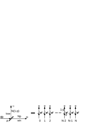
Figure 1: A beam splitter with more reflection than transmission as an implementation of game A in Parrando game paradox.The double-faced box with a dark side and a grey side is the beam splitter. Many uncorrelated photon passing through one beam splitter is equivalent to many single photon passing through many isolated beam splitter.

The game B proposed by Parrondo, Harmer and Abbottparrondo can be interpreted as a single Brownian particle which determines its strategy for the third step based on the winning or losing states two steps earlier. This game can be simulated by computer in a direct way. However it is hard to find ideal correspondence in optical analogy.

We designed an array of beam splitter, and let single classical photon propagate across this array. Here the classical photon is real classical object like small metallic ball, even though I called it photon. Every time the classical photon pass one beam splitter, it is either reflected or transmitted as one, it never split into two halves. We mark the path of transmitted photon by 1 for it is the winning path. The path of reflected photon is labeled by 0. First, we generate the two-step-earlier historical states. The earliest beam is generated by a single beam splitter, it gives one reflection and one transmission. Then we place one beam splitter in each way of the output of the earliest beam splitter to generate the second earlier beams. Each of the two new beam splitters will generate a new pair of transmitted beam and reflected beam. Finally we have four historical states recording the output beams two steps earlier, $\lvert{\textbf{0}_{t-2}\textbf{0}_{t-1}}\rangle$, $\lvert{\textbf{0}_{t-2}\textbf{1}_{t-1}}\rangle$, $\lvert{\textbf{1}_{t-2}\textbf{0}_{t-1}}\rangle$, $\lvert{\textbf{1}_{t-2}\textbf{1}_{t-1}}\rangle$. If the photon is positive in the beginning, the pair of $\lvert{\textbf{0}_{t-2}\textbf{0}_{t-1}}\rangle$ and $\lvert{\textbf{1}_{t-2}\textbf{1}_{t-1}}\rangle$ has positive value for the photon has been reflected even times. While the output of $\lvert{\textbf{0}_{t-2}\textbf{1}_{t-1}}\rangle$ and $\lvert{\textbf{1}_{t-2}\textbf{0}_{t-1}}\rangle$ has negative value since the photon is reflected odd times. In fact, The two-step history game give out a physical understanding to the so-called game paradox. Suppose both the beam splitters at $t-2$ and $t-1$ has a reflection probability $0.8$, the transmission probability is $0.2$. The final gain of path $\lvert{\textbf{0}_{t-2}\textbf{0}_{t-1}}\rangle$ is a positive value, $0.64$. The gain of $\lvert{\textbf{1}_{t-2}\textbf{1}_{t-1}}\rangle$ is $0.04$. The sum of these two positive path, $0.68$, is already larger than $0.5$. Therefore, the three losing games of the beam splitters at $t-2$ and $t-1$ lead to a winning results.

To implement the game B proposed by Parrondo, Harmer and Abbottparrondo , we place the designed beam splitters in game B for each of the four history states. Each of the four states only interact with one special beam splitter $m^{i}_{t}$ at time $t$. Each $m^{i}_{t}$ has a transmission probability of $b_{i}$, and a reflection probability of $(1-b_{i})$. The games rules are summarized as following(Fig. 2),

$$m^{1}_{t}\lvert{\textbf{0}_{t-2}\textbf{0}_{t-1}}\rangle = b_{1}\lvert\textbf{1}_{t}\rangle+e^{i\pi}(1-b_{1})\lvert\textbf{0}_{t}\rangle,$$

$$m^{2}_{t}\lvert{\textbf{0}_{t-2}\textbf{1}_{t-1}}\rangle = b_{2}\lvert\textbf{1}_{t}\rangle+e^{i\pi}(1-b_{2})\lvert\textbf{0}_{t}\rangle,$$

$$m^{3}_{t}\lvert{\textbf{1}_{t-2}\textbf{0}_{t-1}}\rangle = b_{3}\lvert\textbf{1}_{t}\rangle+e^{i\pi}(1-b_{3})\lvert\textbf{0}_{t}\rangle,$$

$$m^{4}_{t}\lvert{\textbf{1}_{t-2}\textbf{1}_{t-1}}\rangle = b_{4}\lvert\textbf{1}_{t}\rangle+e^{i\pi}(1-b_{4})\lvert\textbf{0}_{t}\rangle.$$ (1)

Every history states has an unique destination. For instance, if the photon is reflected by the beam splitters at time $t-2$ and $t-1$, it will meet beam splitter $m^{1}_{t}$. The beam splitters at time $t-2$ and $t-1$ are only used for generating the initial historical states of game B. After the first two-rounds of game B, the newly generated beams out of $m^{i}_{t}$ becomes the history for the next round. Game B can repeat itself on the four designed beam splitters, $m^{i}_{t},\;i=1,2,3,4.$ We denote the four historical states as a vector,

$$\lvert\psi\rangle=[\lvert{\textbf{0}_{t-2}\textbf{0}_{t-1}}\rangle,\lvert{\textbf{0}_{t-2}\textbf{1}_{t-1}}\rangle,\lvert{\textbf{1}_{t-2}\textbf{0}_{t-1}}\rangle,\lvert{\textbf{1}_{t-2}\textbf{1}_{t-1}}\rangle].$$ (2)

The transfer matrix map the historical states one step forward in the direction of time,

$$\lvert\psi_{t-1,t}\rangle = T^{+}\lvert\psi_{t-2,t-1}\rangle.$$ (3)

In this optical analogous system, we can directly read out the transfer matrix $T^{+}$ from Fig. 2,

$$T^{+}=\left[\begin{matrix}e^{i\pi}\mathring{b}_{1}&0&e^{i\pi}\mathring{b}_{3}&0\\ b_{1}&0&b_{3}&0\\ 0&e^{i\pi}\mathring{b}_{2}&0&e^{i\pi}\mathring{b}_{4}\\ 0&b_{2}&0&b_{4}\\ \end{matrix}\right],$$ (4)

where $\mathring{b}_{i}$ is the reflection probability, $\mathring{b}_{i}=1-{b}_{i}$. $T^{+}$ is similar to the matrix given by Parrondo, Harmer and Abbottparrondo , but it is not mathematically equivalent to that matrix. Here we attached a $e^{i\pi}$ phase shifter to every reflection. $T^{+}$ can not be transformed into the matrix in Ref.parrondo through elementary matrix operation. It has different eigenvalue and different eigenstates. We calculated the stationary states $\lvert\psi_{sta}\rangle$ which is invariant under the operation of $T^{+}$, $\lvert\psi_{sta}\rangle=T^{+}\lvert\psi_{sta}\rangle,$ it turns out to be $\lvert\psi_{sta}\rangle=[0,0,0,0].$ While the stationary solution of the matrix in Parrondo-Harmer-Abbott game has complex algebraparrondo .

The transfer operator $T^{+}$ can be physically carried out by properly connecting the output with input. The output of each beam splitter has fixed destination designed by the game rule. We showed the flow chart for implementing the operator $T^{+}$ in the optical network(Fig. 2). The output beam are fused into designed input beams. The photon is trapped in a cyclic optical network. To read out the information of the beam after many rounds, one may disconnect the output from the input. If one use one photon to play game B, one must play it many times to determine the distribution of probability out of each beam splitter. An equivalent way of playing game B is to input a collection of many uncorrelated photons one time, and measure the intensity of output beams.

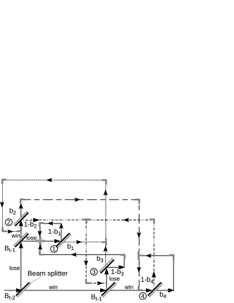
Figure 2: The optical flowchart for implementing the game B. The flow lines with arrow guides the flow of photons. The closed optical loop demonstrate how to realize the transfer matrix for repeating game B.

To get a game paradox in real physical system, we must choose the beam splitters with proper reflection and transmission to lose both game A and game B, and make sure the combination of game A and game B finally wins. The game A is a single beam splitter, if the transmission probability is less than reflection probability, i.e., $p<1/2$, we lose game A. As for game B, Ref. parrondo gave the value of four winning probability to lose the game B in Parrondo-Harmer-Abbott game. However, the matrix in Parrondo-Harmer-Abbott game is not mathematically equivalent to the transfer matrix I used in the optical game B. So their results is not suitable for determining the transmission probability of the four beam splitters here.

I will analyze the optical game B in detail and calculate the distribution of transmission probability for losing this game. First we make a fair history states through $B_{t-2}$ and $B_{t-1}$ in Fig. 2, both of which has transmission probability $p=1/2$. The initial input of $m^{4}_{t}$ is $p_{t-2}p_{t-1}=0.25$. The input of $m^{1}_{t}$ is $(1-p_{t-2})e^{i\pi}(1-p_{t-1})e^{i\pi}=0.25$. The input of $m^{2}_{t}$ and $m^{3}_{t}$ are both $(-0.25)$ due to the phase shifter $e^{i\pi}$. At $m^{1}_{t}$, the photon has probability $b_{1}$ to pass and $1-b_{1}$ to reflect. The transmitted photon will go to $m^{2}_{t+1}$ for it loses at $B_{t-1}$ and wins at $m^{1}_{t}$. The reflected photon at $m^{1}_{t}$ will bent back to $m^{1}_{t+1}$. At $t+1$, the number of photon goes to beam splitter $m^{i}_{t+1}$ are $N_{i,t+1},\;\;(i=1,2,3,4)$,

$$N_{1,t+1} = 0.25e^{i\pi}(1-b_{1})-0.25e^{i\pi}(1-b_{3}),\;\;\;$$

$$N_{2,t+1} = 0.25b_{1}-0.25b_{3},$$

$$N_{3,t+1} = -0.25e^{i\pi}(1-b_{2})+0.25e^{i\pi}(1-b_{4}),\;\;\;$$

$$N_{4,t+1} = -0.25b_{2}+0.25b_{4}.$$ (5)

At time $t+n$, the number of photons to $m^{i}_{t+n}$ is calculated in the same way by operating the transfer matrix $n$ times,

$$\left[\begin{array}[]{l}N_{1,t+n}\\ N_{2,t+n}\\ N_{3,t+n}\\ N_{4,t+n}\end{array}\right]=\left[\begin{array}[]{llll}e^{i\pi}\mathring{b}_{1}&0&e^{i\pi}\mathring{b}_{3}&0\\ b_{1}&0&b_{3}&0\\ 0&e^{i\pi}\mathring{b}_{2}&0&e^{i\pi}\mathring{b}_{4}\\ 0&b_{2}&0&b_{4}\\ \end{array}\right]^{n}\left[\begin{array}[]{l}N_{1,0}\\ N_{2,0}\\ N_{3,0}\\ N_{4,0}\end{array}\right].$$ (18)

$[N_{1,0},N_{2,0},N_{3,0},N_{4,0}]$ is the initial number of photon at $t=0$, here $\vec{N}_{0}=[0.25,-0.25,-0.25,0.25]$. If the photon is reflected in the latest round, we call it a losing path, otherwise, it is winning path. At time $t+n$, the losing paths are $\lvert{\textbf{1}_{t+n-1}\textbf{0}_{t+n}}\rangle$ and $\lvert{\textbf{0}_{t+n-1}\textbf{0}_{t+n}}\rangle$. The winning paths are $\lvert{\textbf{0}_{t+n-1}\textbf{1}_{t+n}}\rangle$ and $\lvert{\textbf{1}_{t+n-1}\textbf{1}_{t+n}}\rangle$. Therefore total number of winning photons are $N_{win}=N_{1,t+n}+N_{4,t+n}$, the losing photons are $N_{lose}=N_{2,t+n}+N_{3,t+n}$. If we want to win the game at $t+n$, then ${\lvert}N_{win}{\lvert}>{\lvert}{N_{lose}}{\lvert}$.

We perform similarity transformation upon both sides of Eq. (18) to diagonalize the transfer matrix without modifying the states vector $\vec{N}$. Each eigenvalue is an algebra equation covered many pages.We denotes them as $[\lambda_{1},\lambda_{2},\lambda_{3},\lambda_{4}]$. The diagonal transfer matrix reads Eq. (18) greatly,

$$\left[\begin{array}[]{l}N_{1,t+n}\\ N_{2,t+n}\\ N_{3,t+n}\\ N_{4,t+n}\end{array}\right]=\left[\begin{array}[]{llll}\lambda^{n}_{1}&0&0&0\\ 0&\lambda^{n}_{2}&0&0\\ 0&0&\lambda^{n}_{3}&0\\ 0&0&0&\lambda^{n}_{4}\\ \end{array}\right]\left[\begin{array}[]{l}N_{1,0}\\ N_{2,0}\\ N_{3,0}\\ N_{4,0}\end{array}\right].$$ (31)

If the distribution of the transmission probability of four beam splitters satisfy the inequality,

$$\lambda^{n}_{1}N_{1,0}+\lambda^{n}_{4}N_{4,0}+\lambda^{n}_{2}N_{2,0}+\lambda^{n}_{3}N_{3,0}>0,$$ (32)

the game wins at time $t+n$. This inequality equation is defined within four dimensional cubic, $\{b_{i}\in[0,1],i=1,2,3,4\}$. We divide this four dimensional cubic into 16 sub-cubic by dividing each $b_{i}$ into two halves, $\{b^{win}_{i}\in(1/2,1],i=1,2,3,4\}$ and $\{b^{lose}_{i}\in[0,1/2),i=1,2,3,4\}$. One way to define a game paradox is the solution of inequity equation (32) exist in the sub-cubic $\{b^{lose}_{i}\in[0,1/2),i=1,2,3,4\}$. Notice that there are four unknown variables but only one inequality equation, the solution space is a three dimensional manifold.

I showed four numerical eigenvalues of the transfer matrix in table 1. $\beta_{k}=\{b_{1},b_{2},b_{3},b_{4}\}$ represents one distribution of the four transmission probability. We calculated four special cases: $\beta_{1}=\{b_{1}=0.2,\;b_{2}=0.2,\;b_{3}=0.2,\;b_{4}=0.2\}$, $\beta_{2}=\{0.8,0.8,0.8,0.8\}$, $\beta_{3}=\{0.2,0.2,0.8,0.8\}$, $\beta_{4}=\{0.8,0.8,0.2,0.2\}$. The corresponding eigenvalue of the transfer matrix is shown in table 1. $\beta_{1}$ represents four losing beam splitters, the corresponding eigenvalue $\lambda_{1}$ is negative, $\lambda_{2}$, $\lambda_{3}$ and $\lambda_{4}$ are almost zero. If we play game B odd times according to $\beta_{1}$, the game loses, while play it even times, the game wins. $\beta_{1}$ is a solution of the inequality equation. $\beta_{2}$ represents four winning beam splitters. It is also one solution of the inequality equation. $\beta_{3}$ and $\beta_{4}$ represents two losing beam splitter and two winning beam splitters. For $\beta_{3}$, $\lambda_{1}$ and $\lambda_{2}$ are imaginary numbers, if we play game even times, the contribution of $\lambda_{1}$ and $\lambda_{2}$ are negative, while $\lambda^{2}_{3}$ and $\lambda^{2}_{4}$ are positive. But the initial input has negative value for $\lambda_{2}$ and $\lambda_{3}$, thus the sum of the four paths are almost zero. The number $0.77$ in the table is the approximation of $0.774597$. There exist very subtle difference between different eigenvalues. The above is just four examples of many solutions. I also checked numerically many other case, there are many solutions within the losing sub-cubic $\{b^{lose}_{i}\in[0,1/2),i=1,2,3,4\}$ which can reach a winning result.

	$\lambda_{1}$	$\vline\lambda_{2}$	$\lambda_{3}$	$\lambda_{4}$
$\beta_{1}$	-0.6	$10^{-19}+i10^{-9}$	$10^{-19}-i10^{-9}$	0
$\beta_{2}$	0.8	$10^{-8}$	-$10^{-8}$	$10^{-17}$
$\beta_{3}$	i0.77	-i0.77	-0.77	0.77
$\beta_{4}$	0.77	-0.77	$10^{-16}$+i0.77	$10^{-16}$-i0.77

Table 1: The four eigenvalues of the transfer matrix for different transmission probability distribution: $\beta_{1}=\{b_{1}=0.2,\;b_{2}=0.2,\;b_{3}=0.2,\;b_{4}=0.2\}$, $\beta_{2}=\{0.8,0.8,0.8,0.8\}$, $\beta_{3}=\{0.2,0.2,0.8,0.8\}$, $\beta_{4}=\{0.8,0.8,0.2,0.2\}$.

In analogy of the combination of two games in Parrondo-Harmer-Abbott gameparrondo , I designed the optical network to combine the optical game A and optical game B here. It is almost the same network for implementing game B(Fig. 2). The beam splitters used for generating historical states for game B are now replaced by the beam splitter of game A. Eight beam splitters are added to play one more round of game B. When the single photon propagates through the array of beam splitters, it shows exactly repeating game A twice followed by two rounds of game B.

First, the photon meet the beam splitter A at time $t-3$(Fig. 3), it has probability $p$ to pass, and probability $(1-p)$ to be reflected. In either case, the output photon will be guided to meet another A-type beam splitter at $t-2$. There will generate four possible states after the two A-type beam splitters at $t-2$. Until now the photon played game A twice to generate the initial historical states for playing game B. At time $t-1$, we place the four beam splitters of game B in each way of the four historical paths. It will generate eight possible paths. Following the game rule between neighboring historical states in game B, we lead each of the eight possible paths into another eight assigned beam splitters at time $t$. So far we played both game A and game B twice.

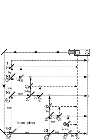
Figure 3: The optical flowchart for playing the combined game in Parrondo-Harmer-Abbott history dependent game. The closed loop repeats the game sequence $A{\rightarrow}A{\rightarrow}B{\rightarrow}B\cdots$.

We input uncorrelated photons one after another into the optical network started with A-type beam splitter at time $t-3$, and counts the total number of photons running out of each B-type beam splitter at time $t$. The total number of transmitted photon is what we win in the combined game. The total number of photons out of the reflection path is the loss. To repeat the cyclic game for $n$ steps by single photon,

$$\overrightarrow{A_{t-3}}\overrightarrow{A_{t-2}}\overrightarrow{B_{t-1}}\overrightarrow{B_{t}}\overrightarrow{A_{t+1}}\overrightarrow{A_{t+2}}\;\cdots\;\cdots\;\overrightarrow{B_{t+n-1}}\overrightarrow{B_{t+n}},$$ (33)

we collect the transmitting path out of the B-type beam splitters at time $t$ into one ultimate path, and fuse all the reflected paths at time $t$ into another ultimate path(Fig. 3). The difference between the two ultimate paths is the net gain. Then we bent the net gain back to the A-type beam splitter at $t-3$. The game, $A\rightarrow{A}\rightarrow{B}\rightarrow{B}$, starts all over again (Fig. 3).

If we do not use single photon to play the game, another equivalent way is to input many uncorrelated photons into beam splitter $A_{-3}$ at the same time. If the transmitted photons out of the eight beam splitters at $t$ is more than those reflected, the game wins. In the language of classical optics, the intensity of transmitted light is stronger than the reflected light. In Fig. 3, we use a positive circle to denote the collection of transmitted light beams, and a negative square to represent the reflected beams.

This optical game is not equivalent to the mathematical game paradox proposed by Parrondo, Harmer and Abbottparrondo . But it can help us to understand those mathematical issues. For physicist, there is no paradox in this optical network. The intensity of reflected light represent exactly the losing probability. The transmitted light measures the winning probability. Even if there are more reflection than transmission at a local beam splitter, as part of the reflected beam can transform into transmitted beam through other beam splitters, it is not paradox if the transmitted beam out of the last round of beam splitters is stronger than the reflected beam.

In fact, one may design much more complicate optical networks for more optical games. We first construct an ultimate optical network that produce stronger transmitted beam than reflected beam. Then we decompose the total network into small networks, and check if the small network generate stronger reflected light than transmitted light. Every beam splitter introduce a variable. For a large network with $m$ beam splitters, the solution of inequality equation of the final gain is distributed in a $m$-dimensional cubic. As the dimension grows, the solution space also expands. One can find many different ways of decomposing the total network, and each sub-network give more reflection than transmission.

III The optical model in analogy of Parrondo’s game

Parrondo’s gameparrondo1996 is the combination of two games. Game A is the same as that in the history-dependent game, it has probability $p$ to win and probability $1-p$ to lose. Game B first check wether the capital is divisible by a number $M$ or not. If the capital can be divided by $M$, it play coin $1$ which has a winning probability $b_{1}$ and a losing probability $1-b_{1}$, otherwise it play coin 2 which has probability $b_{2}$ to win and probability $1-b_{2}$ to loseparrondo1996 .

I will design an optical system to theoretically visualize Parrondo’s game(Fig. 4). First we represent every coin by a beam splitter. The capital is a collection of many classical photons. Game A is realizable by single beam splitter. Game B needs two different beam splitters. The main difficulty of implementing Game B lies in doing the modular algorithm with photons. It is a very complex procedure to check if the number of photon is divisible by $M$ or not. I just use a hexagonal box to represent a fictional machine which can count the number of photons and do the modular computation(Fig. 4). I call this machine a modular beam splitter for it behaves like an effective beam splitter. For example, if $M=5$, an arbitrary number of input photons $N_{input}$ must be one element of the set $\{5k,5k+1,5k+2,5k+3,5k+4\}$. We don’t know wether $N_{input}$ can be divided by 5 or not. The probability for a divisible $N_{input}$ by 5 is $1/5$. $N_{input}$ has a probability $4/5$ of being unable to be divided by $5$. So the $N_{input}$ photons has probability $4/5$ to meet beam splitter $B_{2}$, and has probability $1/5$ to meet $B_{1}$. If we input different number of photons into the modular beam splitter for many times, and denote the sum of these input number as $N_{t}$. The total number of photons collected by $B_{1}$ is $N_{t}/5$. While $4N_{t}/5$ of the total number goes to $B_{2}$. In this sense, the modular beam splitter is equivalent to optical beam splitter. However the modular beam splitter does not add phase shifter on its output beams. An optical beam splitter add a $e^{i\pi}$ on its reflected beam.

We play this optical game B by bending the output of $B_{1}$ and $B_{2}$ back to the initial modular beam splitter, the input capital between the nearest two rounds of game B reads,

$$N_{n+1}=N_{n}\left[\frac{M-1}{M}(2b_{2}-1)+\frac{1}{M}(2b_{1}-1)\right].$$ (34)

Suppose the initial capital is $N_{0}$, then the capital after $k$ rounds of game is,

$$N_{k}=N_{0}\left[\frac{M-1}{M}(2b_{2}-1)+\frac{1}{M}(2b_{1}-1)\right]^{k}.$$ (35)

For the special value of the probability parameter $(b_{1},b_{2})$ and integer $M$ in Ref. harmer , ($M=3$, $b_{2}=1/10$, $b_{1}=3/4$), the capital at the $k$th round of game B is $N_{k}=N_{0}(-11/30)^{k}$. If k is odd number, $N_{k}<0$, the game lost. The game wins for an even number of k. If both $(b_{1},b_{2})$ are larger than $1/2$, the net output capital $N_{k}$ would be constantly positive. For an extreme case of $b_{1}=b_{2}=1$, i.e., $B_{1}$ and $B_{2}$ has zero probability to lose, then $N_{k}=N_{0}[+1]^{k}$. For another extreme case, $b_{1}=b_{2}=0$, $N_{k}=N_{0}[-1]^{k}$ which is positive for $k$ is even. This is because if we input a $(-1)$ into a completely losing game, the output would be $+1$. In fact, a losing game B has two branches of output. If the computer simulation assumes the input capital can only take positive value, the positive branches out of negative input will be eliminated. Only the negative branches is left. Then one will see the capital decreases monotonically. The simulation result of game B as showed in Parrondo’s game is only the negative branch.

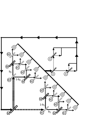
Figure 4: The optical flowchart for implementing Parrondo’s game. The hexagon with $M$ represents the modular beam splitter. The circles with numbers represents the label of beam splitter. Small grey window are the symbol of photon detector.

Parrondo’s gameparrondo1996 is a winning game by periodically repeating game A twice followed by two rounds of game B. Fig. 4 shows the optical flowchart for playing the cyclic game of $B\rightarrow{B}\rightarrow{A}\rightarrow{A}\rightarrow{B}\rightarrow{B}\cdots$. The output of game A is brought back to the input of game B, it forms a closed loop. The game may start from any point in the optical loop. Every transmitted beam out of one modular beam splitter carries a number $1/M$. The weight of the reflected beam from modular beam splitter is $(M-1)/M$. The reflected beam out of $B_{1}$ and $B_{2}$ is attached by an additional phase shifter $e^{i\pi}$ upon their corresponding reflection probability, i.e., $e^{i\pi}(1-b_{j})$. Playing two rounds of game B from single modular beam splitter give out 16 different output path. The final output of each path is calculated by multiplying the weight numbers on all the bonds along this path until it reaches the photon collector(the small grey window in Fig. 4). The input for beam splitter A at the third round is the sum of all the 16 paths. Beam splitter A has reflection probability $p$ and transmission probability $(1-p)e^{i\pi}$. After two rounds of game A, the output flows back to the initial modular beam splitter of game B, then the combined game starts over again.

We can play this game many times using single classical photon, it will give the same results as we play it once using many uncorrelated photon. The game procedure is almost the same as that in the historical game. The main difference is the modular beam splitter. Mathematically there is no difference between dividing $N$ by $M$ and dividing $1$ by $M/N$. All the analyze about reflection and transmission probability holds for single photon. If we do not divide the single photon into many pieces, it is either reflected or transmitted at modular beam splitter. The reflection probability is $(M-1)/M$, and transmission probability is $1/M$. The modular beam splitter does not results in $e^{i\pi}$ phase shift on its reflection.

Generally speaking, Parrondo’s game and Parrondo-Harmer-Abbott history dependent game are the same in my optical analogy, except the transfer matrix in my optical model is not mathematically equivalent to that in their mathematical game. From a physicist’s point of view, both game are reasonable without paradox.

IV Combination of games with long-term memory

We can extend the memory of the game B to $n$-steps of history, $n\geq 3$. Every strategy for the next step depends on the historical states $n$-steps earlier. So we need at least $n$ beam splitters. Every beam coming out of one beam splitter at every step can be clearly marked by reflection beam or transmitted beam. We can use new beam splitter to divide every old beam into two beams—a transmitted beam and a reflected beam. As long as there is no overlap between any newly generated beams, we construct a fractal tree of beam splitters. I will show one extended game with 3-steps of historical memory in the following(Fig. 5).

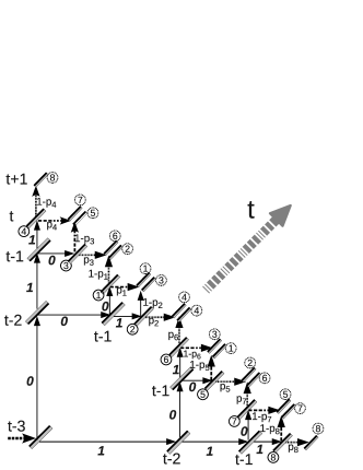
Figure 5: The fractal tree array of beam splitters the game with 3-step memory. The $0$ and $1$ on each bond are label of losing state and winning state. $t-3$ is the origin point. As $t$ goes to infinity, the fractal tree expand larger. The diagram here is the cutoff picture until $t+1$.

Whenever a photon reach a beam splitter, it is either transmitted or reflected. There are eight possible states if the photon pass through three beam splitters one by one. Repeating single photon propagation many times is equivalent to propagate many uncorrelated photons once. A classical Light beams is a collection of many uncorrelated photons. We count the winners by measuring the number of passed photons. The losers are numerated by reflected photons. Every path from the beam splitter at $t-3$ to a beam splitter at $t-1$ ends up with an unique beam splitter marked by binary code sequence(Fig. 5),

$$1_{t} := \lvert{\textbf{0}_{t-3}\textbf{0}_{t-2}\textbf{0}_{t-1}}\rangle,\;\;\;2_{t}:=\lvert{\textbf{0}_{t-3}\textbf{0}_{t-2}\textbf{1}_{t-1}}\rangle,$$

$$3_{t} := \lvert{\textbf{0}_{t-3}\textbf{1}_{t-2}\textbf{0}_{t-1}}\rangle,\;\;\;4_{t}:=\lvert{\textbf{0}_{t-3}\textbf{1}_{t-2}\textbf{1}_{t-1}}\rangle,$$

$$5_{t} := \lvert{\textbf{1}_{t-3}\textbf{0}_{t-2}\textbf{0}_{t-1}}\rangle,\;\;\;6_{t}:=\lvert{\textbf{1}_{t-3}\textbf{0}_{t-2}\textbf{1}_{t-1}}\rangle,$$

$$7_{t} := \lvert{\textbf{1}_{t-3}\textbf{1}_{t-2}\textbf{0}_{t-1}}\rangle,\;\;\;8_{t}:=\lvert{\textbf{1}_{t-3}\textbf{1}_{t-2}\textbf{1}_{t-1}}\rangle.$$ (36)

We introduce a beam splitter operator, $m^{j}_{t}$, to express the action of the beam splitter ${j}_{t}$ at $t$. Beam splitter ${j}_{t}$ let $p_{j}$ of the beam pass, and reflect $1-p_{j}$ of the beam,

$$m^{j}_{t}\lvert{\textbf{s}_{t-3}\textbf{s}_{t-2}\textbf{s}_{t-1}}\rangle=p_{j}\lvert\textbf{1}_{t}\rangle+e^{i\pi}(1-p_{j})\lvert\textbf{0}_{t}\rangle,$$

$$j=\textbf{s}_{t-3}\cdot 2^{2}+\textbf{s}_{t-2}\cdot 2^{1}+\textbf{s}_{t-1}\cdot 2^{0}+1.$$ (37)

Here $j$ corresponds to the number enclosed by a small circle in Fig. 5. Since every beam splitter corresponds to an unique 3-step historical states. For simplicity, we use the sequence of beam splitters at any time $t$ to express the corresponding 3-step historical states before $t$,

$$\psi_{t}=\left[\;1_{t},\;2_{t},\;3_{t},\;4_{t},\;5_{t},\;6_{t},\;7_{t},\;8_{t}\;\right]^{T}.$$ (38)

To replay this 3-step history-dependent game, the beam coming out of every beam splitter at time $t$ must be guided back into the correct beam splitter at $t+1$. The mapping operator from state $\psi_{t}$ to state $\psi_{t+1}$ is

$$T_{{}_{3}}^{+}=\left[\begin{matrix}p_{1}&0&0&0&\mathring{p}_{5}&0&0&0\\ \mathring{p}_{1}&0&0&0&p_{5}&0&0&0\\ 0&\mathring{p}_{2}&0&0&0&\mathring{p}_{6}&0&0\\ 0&p_{2}&0&0&0&p_{6}&0&0\\ 0&0&\mathring{p}_{3}&0&0&0&\mathring{p}_{7}&0\\ 0&0&p_{3}&0&0&0&p_{7}&0\\ 0&0&0&p_{4}&0&0&0&\mathring{p}_{8}\\ 0&0&0&\mathring{p}_{4}&0&0&0&p_{8}\\ \end{matrix}\right],$$ (39)

where $\mathring{p}_{i}$ is the reflection probability attached by a phase shifter, $\mathring{p}_{i}=e^{i\pi}(1-{p}_{i})$. $T_{{}_{3}}^{+}$ is the transfer matrix between the nearest neighboring time point. The states after $n$ rounds of game is reached by operating $T_{{}_{3}}^{+}$ on the initial states $n$ times,

$$\lvert{\textbf{s}_{t+n-3}\textbf{s}_{t+n-2}\textbf{s}_{t+n-1}}\rangle=(T_{{}_{3}}^{+})^{n}\lvert{\textbf{s}_{t-3}\textbf{s}_{t-2}\textbf{s}_{t-1}}\rangle.$$ (40)

$\lvert{\textbf{s}_{t-3}\textbf{s}_{t-2}\textbf{s}_{t-1}}\rangle$ represents the initial input generated by three historical beam splitters. Following the fractal-tree in Fig. 5, every path must pass three beam splitters, $\{m_{t-3},m_{t-2},m_{t-1}\}$(here we use time index to label the same type of beam splitter for simplicity), to reach the beam splitter at time $t$. There are one $m_{t-3}$ beam splitter, two $m_{t-2}$ and four $m_{t-1}$ beam splitters. The initial intensity of the beam can be read out by direct inspection of Fig. 5,

$$P_{1} = {\mathring{p}_{{}_{t-3}}\mathring{p}_{{}_{t-2}}\mathring{p}_{{}_{t-1}}},\;\;\;P_{2}=\mathring{p}_{{}_{t-3}}\mathring{p}_{{}_{t-2}}p_{{}_{t-1}},$$

$$P_{3} = {\mathring{p}_{{}_{t-3}}p_{{}_{t-2}}\mathring{p}_{{}_{t-1}}},\;\;\;P_{4}={\mathring{p}_{{}_{t-3}}p_{{}_{t-2}}p_{{}_{t-1}}},$$

$$P_{5} = {p_{{}_{t-3}}\mathring{p}_{{}_{t-2}\textperiodcentered}\mathring{p}_{{}_{t-1}}},\;\;\;P_{6}={p_{{}_{t-3}}\mathring{p}_{{}_{t-2}}p_{{}_{t-1}}},$$

$$P_{7} = {p_{{}_{t-3}}p_{{}_{t-2}}\mathring{p}_{{}_{t-1}}},\;\;\;P_{8}={p_{{}_{t-3}}p_{{}_{t-2}}p_{{}_{t-1}}}.$$ (41)

To play a fair game, the initial capital of eight paths, i.e., the initial number of photons in eight paths, must be the same. Thus we assign the same transmission probability to the three historical beam splitter, i.e., $(P_{t-3}=P_{t-2}=P_{t-1}=1/2)$.

If we investigate the states of game after finite number of rounds, it is convenient to diagonalize the transfer matrix $T_{{}_{3}}^{+}$ by performing similarity transformation upon Eq. (40). Then $(T_{{}_{3}}^{+})^{n}$ is expressed by the eight eigenvalues $\lambda^{n}_{i},(i=1,2,3,\cdots,8)$,

$$(T_{{}_{3}}^{+})^{n}=Diag[\lambda^{n}_{1},\lambda^{n}_{2},\lambda^{n}_{3},\lambda^{n}_{4},\lambda^{n}_{5},\lambda^{n}_{6},\lambda^{n}_{7},\lambda^{n}_{8}].$$ (42)

I calculated some numerical value of these eigenvalues for five special cases(2): (1) $\beta_{1}$, eight beam splitters all lose; (2) $\beta_{2}$, eight beam splitters all win; (3) $\beta_{3}$, four beam splitters lose, the other four win; (4) $\beta_{4}$, six beam splitters lose, the other two win; (5) $\beta_{5}$, two beam splitters lose, the other six win. The corresponding eigenvalue are shown in table 3. The zeroes in the box are approximation of $10^{-10}\sim 10^{-19}$. The eigenvalue for the five special cases all includes complex number, and neighboring complex eigenvalue are conjugate. $\lambda_{7}$ and $\lambda_{8}$ are approximately zero. We study the all-losing case $\beta_{1}$ as an example. The imaginary part of are $\lambda_{1}$ and $\lambda_{1}$ are $88$ times larger than their corresponding real part. We take their real part as zero. Then we play the game 2 times with $\beta_{1}$, the total gain is calculated by $G=\sum^{8}_{i=1}P_{i}\lambda^{2}_{i}=0.05355$, so the final game wins even if all the eight beam splitters loses.

	$p_{1}$	$p_{2}$	$p_{3}$	$p_{4}$	$p_{5}$	$p_{6}$	$p_{7}$	$p_{8}$
$\beta_{1}$	0.2	0.2	0.2	0.2	0.2	0.2	0.2	0.2
$\beta_{2}$	0.8	0.8	0.8	0.8	0.8	0.8	0.8	0.8
$\beta_{3}$	0.2	0.2	0.2	0.2	0.8	0.8	0.8	0.8
$\beta_{4}$	0.2	0.2	0.2	0.2	0.2	0.2	0.8	0.8
$\beta_{5}$	0.8	0.8	0.8	0.8	0.8	0.8	0.2	0.2

Table 2: The five special distribution of the eight beam splitter’s transmission probability.

	$\lambda_{1}$	$\vline\lambda_{2}$	$\lambda_{3}$	$\lambda_{4}$	$\lambda_{5}$	$\lambda_{6}$	$\lambda_{7}$	$\lambda_{8}$
$\beta_{1}$	-0.01	-0.01,	0.74	-0.6	0.57	-0.29	0	0
Im	i 0.88	-i0.88	0	0	0	0	0	0
$\beta_{2}$	-0.42	-0.42	0.83	0.83	0.6	0.19	0	0
Im	i 0.76	-i0.76	i 0.02	-i 0.02	0	0	0	0
$\beta_{3}$	0.94	0.86	-0.33	0.33	-0.07	-0.07	0	0
Im	0	0	i 0.71	-i 0.71	i0.33	-i0.33	0	0
$\beta_{4}$	0.9	-0.02	-0.02	0.76	-0.63	0	0	0
Im	0	-i0.85	i 0.85	0	0	0	0	0
$\beta_{5}$	-0.48	-0.48	0.59	0.59	0.77	0	0	0
Im	i0.66	-i0.66	i 0.5	0	0	0	0	0

Table 3: The eight corresponding eigenvalues with respect to the transmission probability distribution in table 2. The zeroes in small boxes are approximation of $10^{-10}\sim 10^{-19}$. $Im$ indicate the imaginary part of the eigenvalue.

A more geometric way of visualizing this game is to draw a fractal tree of history. Every bond on the tree has a number representing reflection or transmission. We follow each path from the origin point to the end, and multiply all the numbers on the bond along this path, then we get the gain of this path. The sum of all different paths give the total gain. For example, there are many future paths starting with $4_{t}$ at time $t$. These future paths are given by the transfer matrix $T_{{}_{3}}^{+}$. In Fig. 6, we showed the fractal tree of the paths started from $4_{t}$ until $t+4$. Any path is marked by an unique binary code sequence. Every three nearest neighboring binary code indicates one historical states. For instance, the binary sequence

$$\textbf{0}_{t-3}\textbf{1}_{t-2}\textbf{1}_{t-1}\textbf{1}_{t}\textbf{0}_{t+1}\textbf{0}_{t+2}\textbf{1}_{t+3}$$ (43)

is equivalent to a sequences of 3-step states,

$$\lvert{\textbf{0}_{t-3},\textbf{1}_{t-2},\textbf{1}_{t-1}}\rangle\rightarrow\lvert{\textbf{1}_{t-2},\textbf{1}_{t-1},\textbf{1}_{t}}\rangle\rightarrow\lvert{\textbf{1}_{t-1},\textbf{1}_{t},\textbf{0}_{t+1}}\rangle$$

$$\rightarrow\lvert{\textbf{1}_{t},\textbf{0}_{t+1},\textbf{0}_{t+2}}\rangle\rightarrow\lvert{\textbf{0}_{t+1},\textbf{0}_{t+2},\textbf{1}_{t+3}}\rangle.$$ (44)

In mind of the unique decimal labeling of the beam splitter after the eight historical states, Eq. (IV), we get the sequence of beam splitters with different transmission and reflection,

$$4_{t}\rightarrow 8_{t+1}\rightarrow 7_{t+2}\rightarrow 5_{t+3}\rightarrow 2_{t+4}.$$ (45)

Every sequence like the above corresponds to an unique path in the fractal-tree network(Fig. 6). This path is labeled by $57$ (Fig. 6) which is the decimal mapping of the sequence of binary code Eq. (43),

$$0\cdot 2^{6}+1\cdot 2^{5}+1\cdot 2^{4}+1\cdot 2^{3}+0\cdot 2^{2}+0\cdot 2^{1}+1\cdot 2^{0}.$$ (46)

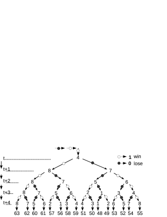
Figure 6: The decimal labeling of all the paths starting from beam splitter 4 until time $t+4$. The small black disc indicates the reflection beam. The small white disc represent the transmission beam. The numbers within $1\sim 8$ after each black or white disc are the label of the beam splitter in game B.

For a given time $t^{\prime}$, the path ended up with $\textbf{1}_{t^{\prime}}$ is winning path. The paths ended up with $\textbf{0}_{t^{\prime}}$ are losing paths. The gain(loss) of winning(losing) path is calculated by the scalar product of the probability at every beam splitter along the path. We calculate the profit of the path sequence Eq. (43) until $t+3$ as an example. We denote the number of photons of at beam splitter $4_{t}$ at time $t$ as $N_{0}$. $N_{0}$ is the ultimate result of the historical path before $t$. Following the path $\textbf{1}_{t}\textbf{0}_{t+1}\textbf{0}_{t+2}\textbf{1}_{t+3}$, $N_{0}{p}_{4}$ of the $N_{0}$ photons will pass beam splitter $4_{t}$. So the gain of this path at time $t$ is $G_{t}=N_{0}{p}_{4}$. At $t+1$, the photons will be reflected by the beam splitter $8_{t+1}$. The number of reflected photons at $t+1$ is $G_{t+1}=G_{t}\mathring{p}_{8}=N_{0}{p}_{4}\mathring{p}_{8}$, where $\mathring{p}_{8}=1-{p}_{8}$ is the reflection probability of $8_{t+1}$. Following the same calculation, the photons will be reflected at $7_{t+2}$ and transmitted through $5_{t+3}$. The final gain of the path $4_{t}8_{t+1}7_{t+2}5_{t+3}$ is

$$G^{(57)}_{t+3}=N_{0}{p}_{4}\mathring{p}_{8}\mathring{p}_{7}{p}_{5}.$$ (47)

This is only the gain of path $57$ until time $t+3$. There are $2^{7}=128$ independent paths at $t+3$, part of which is shown in Fig. 6. To find out wether the total game is winning or losing until time $t+3$, we must calculate the profit of all the paths, and compare the ultimate number of transmitted photon and the number of reflected photons. If the transmitted photon is more than the reflected ones, the game wins, otherwise the game loses.

The total number of output paths grows following $2^{t}$ as time goes on. If we investigate the behavior of the game in the long run, it is better to use differential equations with continuous time. Every beam splitter at time $t$ corresponds to an unique three-beam splitter sequence in the latest history. Thus if one knows the label of beam splitter, one can deduce the information about winning or losing in the latest three steps of game in history. For instance, if the label of four beam splitters at time $t$ are $\left\{\;{1},\;{3},\;{5},\;{7}\right\},$ the game along the four paths at time $t-1$ is losing. For the paths ended up with beam splitters $\left\{\;{2},\;{4},\;{6},\;{8}\right\}$ at time $t$, the game at time $t-1$ is winning. We summaries the eight beam splitters into a vector in Eq. (38). The transfer operator $T^{+}_{{}_{3}}$ maps a vector $\psi_{t}$ to a new vector $\psi_{s}(t+1)$ at $t+1$. The new vector of eight beam splitters bear the same meaning as that at time $t$, while the time index increased one step further. Within a longer period, we take the time interval as continuous variable so that the difference between neighboring states in history can be denoted as a derivative, $\psi_{t+1}-\psi_{t}={\partial}_{t}\psi_{t}$. Then we map the equation of transfer operator into a differential equation,

$$\frac{\partial}{\partial{t}}\psi_{t} = [{T}_{{}_{3}}^{+}-I]\psi_{t}.$$ (48)

where $[{T}_{{}_{3}}^{+}-I]$ play the role of Hamiltonian. $I$ is the identity matrix. A similarity transformation performed upon both sides of this differential equation can diagonalize the Hamiltonian operator by keeping the equation invariant. Properly choosing reflection and transmission probability of the eight beam splitter, one can get an invariant vector which keep the same value all the time. This static solution is the eigenfunction of equation ${T}_{{}_{3}}^{+}\psi_{t}=\psi_{t}$,

We can design similar flowchart to implement the eight dimensional transfer operator as that for the two-step optical game B. The transfer operator redistribute the beams among different beam splitters following the dynamic equation (48). The beams passing through some beam splitter may get stronger, while others may become weaker. The time dependent distribution is the solution of dynamic equation (48). Exactly diagonalizing the matrix $[T_{{}_{3}}^{+}-I]$, we derived the eigenvalues of the eight beam splitters, $\left\{\;E_{j},\;\;j=1,2,3,\cdots,8\;\right\}.$ Each eigenvalue is a heavy algebra equation of the eight unknown transmission probability. The solution of the dynamic equation Eq. (48) has the following form,

$$j(t)=P_{j}\exp[{E_{j}t}],\;\;\;j=1,2,3,..,8.$$ (49)

$P_{j}$ is the initial intensity of light beams at time $t=0$.

We decompose the eigenvalues into real part and imaginary part, $E_{j}=Re_{j}+i\;Im_{j}$. The real part determines wether the solution diverges or decay to zero as time goes to infinity. The imaginary part governs the oscillation of the probability of finding certain beam splitter at time $t$. The fractal tree game in Fig. 5 shows $\{{1}(t+1),{3}(t+1),{5}(t+1),{7}(t+1)\}$ collect winning beams at time $t+1$, while $\{{2}(t+1),{4}(t+1),{6}(t+1),{8}(t+1)\}$ absorb the losing beams. Thus the total gain of the game at time $t$ is the sum of four winning paths— $\{{1},{3},{5},{7}\}$,

$$G(t) = \sum_{j}P_{j}\exp[{E_{j}t}],\;\;\;j=1,3,5,7.$$ (50)

The total loss until time $t$ is

$$L(t) = \sum_{k}P_{k}\exp[{E_{k}t}],\;\;\;k=2,4,6,8.$$ (51)

For a winning game, the gain is lager than the loss, ${\lvert}G(t)\lvert>{\lvert}L(t)\lvert$. For a losing game, ${\lvert}G(t)\lvert<{\lvert}L(t)\lvert$. The inequality equation only provide one constraint on the eight unknown variables, i.e., $G(t):=G(t,p_{1},p_{2},p_{3},p_{4},p_{5},p_{6},p_{7},p_{8})$. Thus there are many different ways to choose proper transmission probability for each of the eight beam splitters. For example, we introduce some equations by hand,

$$Re[{E_{j}}] \geq 0,\;\;\;Im[{E_{j}}]=0,\;\;\;\;j=1,3,5,7,$$

$$Re[{E_{k}}] \leq 0,\;\;\;Im[{E_{k}}]=0,\;\;\;\;k=2,4,6,8.$$ (52)

These equations makes the winning beams grow stronger, the losing beams gets weaker. The zero imaginary part eliminated the oscillation.

The above procedure of designing optical network for game paradox has a straight extension to the $n$-step history-dependent game. However only classical game on network can be analyzed by the same strategy of analyzing the three-step history-dependent game paradox. By classical game, I mean every path has a definite state of wining or losing. If there exist closed path in network, two beams are allowed to inject into the same beam splitter from the opposite surface of the mirror, then the transmitted beams from one side may fuse into the reflected beam from the other side. In that case, we have to draw a double line—one winning line and one losing line—to label the path.

However, the beam splitter in the loop network does not have unique transmission probability which can be determined self-consistently by the same historical mapping rule. For example, if we construct a closed square by placing a single beam splitter at $t+1$ to meet the other three beam splitters ${3}_{t}\rightarrow{m}_{t-1}\rightarrow{4}_{t}$ in Fig. 5, it can not simultaneously satisfy the mapping rule of the vertical path and the horizontal path. The vertical path leads to ${5}_{t}$, the horizontal path leads to ${7}_{t}$. One way to keep the historical mapping rule is popping into the third spatial dimension: place ${5}_{t}$ on top of ${7}_{t}$ at the same lattice site of two dimensions.

In fact, we can design more general game paradox by abandoning the historical mapping rule. First, we construct a network of beam splitters, and define its output channel and input channel. Second, the winning capital is the sum of all the transmitted beams. The losing is the sum of all reflected channels. Finally, we find the proper transmission probability of each beam splitter so that the total winning capital is larger than the losing channel. A special exemplar design is shown in Fig. 7 (a) which includes only four beam splitters. Each beam splitter $j$ has the probability $b_{j}$ to win and probability $1-b_{j}$ to lose, $j=0,1,2,3$. We start from game $0$, every time the games loses, we switch to next game, $0\rightarrow 1\rightarrow 2\rightarrow 3\rightarrow 0\cdots$. The winning beam are collected by the output rhombus. Even if each beam splitter has very small transmission probability, $(b_{j}=\epsilon_{j}\ll 1,\;\;\;j=0,1,2,3,)$ after a enough long time, all the photons will be collected by the output. This is winning game in the end.

$\begin{array}[]{c@{\hspace{0.25in}}c}\vspace{-0.1cm}\includegraphics[width=95.39693pt]{star.eps}\hfil\hskip 18.06749pt&\includegraphics[width=95.39693pt]{tra4.eps}\\ \mbox{(a)}\hfil\hskip 18.06749pt&\mbox{(b)}\\ \end{array}$

Figure 7: (a) A loops game with four beam splitters. All reflection beams are transfer into transmission beam. (b) The loop game on square lattice. Each bond is the overlap of many transmission and reflection.

The history tree for playing many rounds of the square game with four beam splitters in Fig. 7 (a) also have a fractal structure. As long as we can distinguish the reflected beam with the transmitted at each round of game, every path in history has an unique label. Whenever the beam flows into a beam splitter at some lattice site at certain time, the beam splitter must make another copy of itself and split into two different paths to separate the overlapped reflection beam and transmission beam. The history tree of the game becomes a huge fractal network, especially when we extend this square game into a square lattice of many beam splitters.

In mind of the fact we are dealing with the beam of probability flow instead of physical beams so far, we can design a game of real light beam on square lattice of many beam splitters like Fig. 7 (b). In that case, we can not distinguish reflection beam from transmission beam passing through each bond. Firstly, one has to define the output beam splitter and input beam splitter along the boundary. The we inject $N$ photons into the input beam splitter, and collect the output photon. If the output number of photons is larger than $N/2$, the game is winning, otherwise, the game is lost. The lattice structure enclosed by the boundary may be very complex. To create a physical game paradox, we cut the whole network into two or more sub-networks in a proper way so that there are less transmitted photons than reflected photons through each sub-network. But as a whole network, the transmitted photon is more than those reflected ones.

V History-entangled game

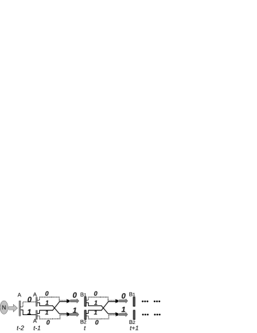
Figure 8: The history-entangled game with two beam splitter in game B. The grey bar represents beam splitters. Three A-type beam splitters are used for generating initial historical states.

If the game ask the player to choose its strategy for the next step according to historical record, but the player lost some historical information. In this case, the player will select all possible historical states to determine its strategy. The final output the game not only depends on historical states, but also depends how the player organize those states. I call this kind of game a history-entangled game.

I take a Brownian particle with incomplete memory as player. The particle first travel across three identical A-type beam splitter to generate four initial history states(Fig. 8). The transmission probability of $A$-type beam splitter is $p_{{}_{A}}$. Its reflection probability is $(1-p_{{}_{A}})$. If we have capital $N$ in the beginning, then the output capital of the four beams after A-beam splitters are(Fig. 8)

$$C_{00} = N(1-p_{{}_{A}})^{2},\;\;\;\;C_{11}=Np_{{}_{A}}^{2},$$

$$C_{01} = C_{10}=N(p^{2}_{{}_{A}}-p_{{}_{A}}).$$ (53)

To make a fair game without dependence on initial condition, we choose exactly $p_{{}_{A}}=1/2$ for symmetric states, then $C_{00}=C_{11}=0.25$, $C_{01}=C_{01}=-0.25$.

When the particle meet beam splitter $B_{1}$ and $B_{2}$ at the third step, it only remembers wether the past two rounds of game has the same result or different result. For instance, if it remembers that it won only once during the latest two rounds of game, but it does not remember in which round it wins. If it wins or loses two rounds, the only memory kept in its mind is the results of the two rounds are the same. The strategy of the particle is to put the output of $\lvert{\textbf{0}_{t-2}\textbf{0}_{t-1}}\rangle$ and $\lvert{\textbf{1}_{t-2}\textbf{1}_{t-1}}\rangle$ together, and submit them to $B_{1}$ beam splitter. The output of $\lvert{\textbf{0}_{t-2}\textbf{1}_{t-1}}\rangle$ and $\lvert{\textbf{1}_{t-2}\textbf{0}_{t-1}}\rangle$ are combined into $B_{2}$ beam splitter(Fig. 8).

There are two different ways to mix two historical states. One way is adding them up so that switching the two beams arrives at the same state. We called it symmetric state,

$$\lvert{\phi_{1,t}}\rangle = \lvert{\textbf{0}_{t-2}\textbf{0}_{t-1}}\rangle+\lvert{\textbf{1}_{t-2}\textbf{1}_{t-1}}\rangle,$$

$$\lvert{\phi_{2,t}}\rangle = \lvert{\textbf{0}_{t-2}\textbf{1}_{t-1}}\rangle+\lvert{\textbf{1}_{t-2}\textbf{0}_{t-1}}\rangle.$$ (54)

The other way is subtracting one beam from another beam. If we switch the position of the two states, it will generate a $(-1)$ sign on the original state. We call it antisymmetric state,

$$\lvert{\psi_{1,t}}\rangle = \lvert{\textbf{0}_{t-2}\textbf{0}_{t-1}}\rangle-\lvert{\textbf{1}_{t-2}\textbf{1}_{t-1}}\rangle,$$

$$\lvert{\psi_{2,t}}\rangle = \lvert{\textbf{0}_{t-2}\textbf{1}_{t-1}}\rangle-\lvert{\textbf{1}_{t-2}\textbf{0}_{t-1}}\rangle.$$ (55)

Both the symmetric state and antisymmetric state are similar to the well known Bell state in quantum mechanics. However I just use Dirac bracket to denote state for convenience, there is no quantum state here. The symmetric states is comprehensible from the point view of single Brownian particle. It is also convenient for computer simulation. Since both $\lvert{\textbf{0}_{t-2}\textbf{0}_{t-1}}\rangle$ and $\lvert{\textbf{1}_{t-2}\textbf{1}_{t-1}}\rangle$ will meet $B_{1}$, it is natural to add up their probability. The anti-symmetric states can be simulated by computer, but it is hard to explain physically by probability theory of conventional Brownian particle. We keep the antisymmetric state as a choice of particle’s strategy.

We first study the long term behavior of the symmetric state in by repeating game B. $B_{1}$ take $\lvert{\phi_{1,t}}\rangle$, let $b_{1}$ of the input pass and reflect $(1-b_{1})$. $\lvert{\phi_{2,t}}\rangle$ will meet beam splitter $B_{2}$. There also generate a pair of transmission and reflection at $B_{2}$. When the four output of $B_{1}$ and $B_{2}$ at $t$ go to the next round game at another pair of $B_{1}$ and $B_{2}$ at $t+1$, the particle began to take the output at $t$ as historical states to reorganize the latest 2-step history following the same game rule. It view $\lvert{\phi_{1,t}}\rangle$ as a losing state $\lvert{\textbf{0}_{t}}\rangle$, and $\lvert{\phi_{2,t}}\rangle$ is winning state $\lvert{\textbf{1}_{t}}\rangle$(Fig. 8). Repeating the pair of $B_{1}$ and $B_{2}$ will generate a sequence of the pair of states,

$$\lvert\phi_{t}\rangle=[\lvert{\phi_{1,t}}\rangle,\lvert{\phi_{2,t}}\rangle]^{T}.$$ (56)

The transfer matrix mapping every state vector $\lvert\phi_{t}\rangle$ one step forward into $\lvert\phi_{t+1}\rangle$ is

$$T_{\phi}^{+}=\left[\begin{matrix}e^{i\pi}(1-{b}_{1})&b_{2}\\ b_{1}&e^{i\pi}(1-{b}_{2})\\ \end{matrix}\right].$$ (57)

If game B is played so many times that the lifetime of the whole game is almost infinite comparing with single round of game, we take state function as a continuous distribution, and write the difference equation as the derivative of $\lvert{\phi}_{t}\rangle$ with respect to time, $\lvert\phi_{t+1}\rangle-\lvert\phi_{t}\rangle={\partial}_{t}\lvert\phi_{t}\rangle$. Then the discrete equation, $\lvert{\phi}_{t+1}\rangle=T^{+}\lvert{\phi}_{t}\rangle,$ is equivalently mapped into the differential equation, ${\partial_{t}}\lvert{\phi}\rangle=[T_{\phi}^{+}-I]\lvert{\phi}\rangle.$ As the probability element in the transfer matrix have no dependence on time, we can diagonalize the composite matrix $[T_{\phi}^{+}-I]$ directly to determine the long term behavior of the states. The two eigenvalues of the composite matrix are $E_{1}=-2,E_{2}=-2+b_{1}+b_{2}$, so the solution of this differential equation is.

$$\lvert{\phi_{1}}\rangle=P_{0}\exp[{-2t}],\;\;\lvert{\phi_{2}}\rangle=P_{0}\exp[{(-2+b_{1}+b_{2})t}].$$ (58)

$P_{0}$ is the initial capital at time $t=0$. The total gain at time $t$ is

$$G(t)=P_{0}(2b_{1}-1)e^{-2t}-P_{0}(2b_{2}-1)e^{(-2+b_{1}+b_{2})t},$$ (59)

Here the absolute value of initial input capital is $P_{0}=0.25$. The initial input is determined by $C_{00}=C_{11}=0.25$ and $C_{01}=C_{01}=-0.25$. The total gain $G(t)$ at time $t=6$ is plotted in Fig. 9 (a). As time goes to infinity, the total gain approaches to zero, $\lim_{t\rightarrow\infty}G(t)=0$. When both game $B_{1}$ and $B_{2}$ wins, the combined game loses. The gain function in Fig. 9 (a) drops to negative in the region $b_{2}>1/2,\;b_{1}>1/2$. When $b_{2}<1/2$, the total gain is positive and increasing as $b_{1}$ increases from $0$ to $1$. Thus if $B_{1}$ and $B_{2}$ loses, the game can still win. If beam splitter $B_{1}$ wins at $b_{1}=1$, while $b_{2}$ increase from $0$ to $0.32$, the gain is positive and reaches its maximal point at $b_{2}=0.32$. As $b_{2}$ continuous to increase, the gain drops to zero and finally becomes negative.

$\begin{array}[]{c@{\hspace{0.15in}}c}\vspace{-0.1cm}\includegraphics[width=99.73074pt]{gboson.eps}\hfil\hskip 10.84006pt&\includegraphics[width=99.73074pt]{gfermi.eps}\\ \mbox{(a)}\hfil\hskip 10.84006pt&\mbox{(b)}\\ \end{array}$

Figure 9: (a) The final gain of symmetric states at t=6. Here we chose $P_{0}=1$ in the computation for convenience. (b) The final gain of antisymmetric states at time t=10.

The output of antisymmetric states is much more complex than the output of the symmetric states. If two Brownian particle has no correlation, playing the two rounds of game twice using one Brownian particle is equivalent to playing the two rounds of game only once using two separate Brownian particle. This indeed is true for the symmetric states. But to play the antisymmetric states, there must exist a correlation between the two Brownian particles. Suppose two Brownian particle meet beam splitters $A_{t-2}$ and $A_{t-1}$, one wins twice, the other lose twice. When they get into $B_{1}$, either the double winning particle or the double losing one must flip a sign to its capital. One particle must check the sign of the other one to determine its own sign. If play the antisymmetric state using single Brownian particle, there exist a historical correlation between the two-winning-step at one time and the two-losing-step at another time. If the single Brownian particle wins twice, when it meets $B_{1}$, it can not decide its own sign. So it has to search the history record for the nearest two-losing-step to check its sign. The computer can flip a sign of a number in an easy way. In physics, it is a complex design to add a $\exp[i\pi]$ phase shift on a real photon, besides this phase shift can only be added after it transmitted through two nearest neighboring beam splitters. One may use optical medium to delay the photon. However, if we play many rounds of game, the number of optical medium will exponentially increase to infinity.

The long term behavior of the antisymmetric state is significantly different from symmetric states. The game rule of beam splitter $B_{1}$ and $B_{2}$ for antisymmetric states is the same as that for symmetric states,

$$B_{1}\lvert{\psi}\rangle = b_{1}\lvert\textbf{1}_{t}\rangle+e^{i\pi}(1-b_{1})\lvert\textbf{0}_{t}\rangle,$$

$$B_{2}\lvert{\psi}\rangle = b_{2}\lvert\textbf{1}_{t}\rangle+e^{i\pi}(1-b_{2})\lvert\textbf{0}_{t}\rangle.$$ (60)

The equation of motion for the antisymmetric state vector, $\lvert{\psi}\rangle:=[\;\lvert{\psi_{1}}\rangle,\;\lvert{\psi_{2}}\rangle\;]^{T},$ is ${\partial_{t}}\lvert{\psi}\rangle=[T_{\psi}^{+}-I]\lvert{\psi}\rangle.$ The transfer matrix between two nearest neighboring historical states is

$$T_{\psi}^{+}=\left[\begin{matrix}e^{i\pi}(1-{b}_{1})&-b_{2}&\\ b_{1}&-e^{i\pi}(1-{b}_{2})&\\ \end{matrix}\right].$$ (61)

$[T_{\psi}^{+}-I]$ may be view as an effective Hamiltonian which has two eigenvalues,

$$E_{-} = \frac{1}{2}(-2-b_{2}+b_{1}-\sqrt{\Delta}),$$

$$E_{+} = \frac{1}{2}(-2-b_{2}+b_{1}+\sqrt{\Delta}).$$ (62)

where $\Delta=(2+b_{2}-b_{1})^{2}-8b_{2}$ is the gap between two levels. Both the two eigenvalues are negative(Fig. 10). So the two antisymmetric states will converge to zero when time goes to infinity. This a draw game in the long run. But its output in finite time domain could be winning, losing, or oscillating. We analyze the final gain,

$$G(t)=(2b_{1}-1)\lvert{\psi_{1}}\rangle-(2b_{2}-1)\lvert{\psi_{2}}\rangle,$$ (63)

from the time-dependent solution of the two antisymmetric states,

$$\lvert{\psi_{1}}\rangle = P_{0}\exp[\frac{1}{2}(-2-b_{2}+b_{1}-\sqrt{\Delta})t],$$

$$\lvert{\psi_{2}}\rangle = P_{0}\exp[\frac{1}{2}(-2-b_{2}+b_{1}+\sqrt{\Delta})t].$$ (64)

The gain function $G(t)$ has three different branches according to the gap $\Delta$.

(1) If $b_{2}=2-2\sqrt{2}\sqrt{b_{1}}+b_{1},$ then $\Delta=0$, two states become degenerated. In the degenerated states, if $b_{1}>b_{2},$ the game wins, otherwise the game loses. Notice that the results only depends on relative ratio between $b_{1}$ and $b_{2}$, even both $b_{1}$ and $b_{2}$ loses, i.e., $b_{1}<1/2$ and $b_{2}<1/2$, the game can still be winning as long as $b_{1}>b_{2}$. On the other hand, if both $b_{1}>1/2$ and $b_{2}>1/2$, the game can also loses if $b_{1}<b_{2}$. There also exist others case, such as one of the two game loses, the total game loses or wins.

(2) If $b_{2}<2-2\sqrt{2}\sqrt{b_{1}}+b_{1},$ the gap is positive $\Delta>0$. The game $b_{2}$ has to lose to make a winning combined game. In the winning region, when $b_{1}$ increases from $0$ to $1$, the gain decreases(Fig. 9). Thus $b_{1}$ also inclined to lose to win the combined game.

(3) If $b_{2}>2-2\sqrt{2}\sqrt{b_{1}}+b_{1},$ the gap is negative, $\Delta<0$. In this region, the two game can not lose simultaneously. When $b_{1}$ loses, $b_{2}$ is always larger than $1/2$. If $b_{2}$ lose, $b_{1}$ slide into the winning region. There is only one point of draw game, $b_{1}=b_{2}=1/2$. However, this region allows the two game to win simultaneously, while the final gain of the combined game does not always win. $G(t)$ oscillates between winning and losing(Fig. 10 (b)). Although the gain is not real number but a imaginary number, in some sense, we still call this a game paradox since combining two winning game give a losing result.

$\begin{array}[]{c@{\hspace{0.15in}}c}\vspace{-0.1cm}\includegraphics[width=95.39693pt]{eigen.eps}\hfil\hskip 10.84006pt&\includegraphics[width=104.07117pt]{oscillator.eps}\\ \mbox{(a)}\hfil\hskip 10.84006pt&\mbox{(b)}\\ \end{array}$

Figure 10: (a) The two eigenvalues of the transfer matrix for antisymmetric states,$E_{-}$ and $E_{+}$. They are both negative. (b) The final gain of antisymmetric states at t=17 within the oscillating region.

The different behavior of the final gain between symmetric states and antisymmetric states implies antisymmetric states is much more efficient to win the global game by losing every local games. For a history dependent game with long term memory, similar antisymmetric state can be constructed following the same strategy. The dimension of probability variables will grows higher. There is much freedom for one to design various different game paradox.

VI Optical game as analogy of Brownian ratchets and many body physics

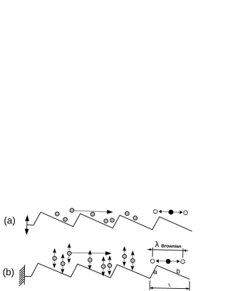
Figure 11: (a) The periodic potential is turned on and off. (b) The periodic potential is constantly presented. While the Brownian particles as a whole is in and out of the potential periodically or randomly.

A classical Brownian particle trapped in a periodic potential shows random motion, no matter the local potential well is symmetric or asymmetric. If the periodic potential with asymmetric local potential is turned on and off periodically, (Fig. 11 (a)), the Brownian particle would move in one directionrousselet . An equivalent way to see this phenomena is to fix the periodic potential but let all the Brownian particles together approach to the potential and leave there quickly(Fig. 11 (b)). This point of view describes the same thing by placing the static observer of reference coordinates on the potential well. Thus Brownian particles move to the right too.

Every asymmetric potential well is analogous to a beam splitter. When the particle hit the potential well, it tends to stay in a lower potential point. If it collides with bond $b$ in Fig. 11 (b), moving to the right is the dominant motion. When it hits bond $a$, it moves to the left(Fig. 11 (b)). Switching the potential on and off in a periodic way in fact is equivalent to generate a standing wave of Brownian particles upon a static potential. In one dimension, Brownian particle has spontaneous random motion along the length of the periodic potential. If we ignore the collision between different Brownian particles, one Brownian particle represents one propagating wave. As a rough phenomenological description, if a Brownian particle can cover an average distance $\lambda_{Brownian}$ during one period of oscillation, $\Delta{T}$, we define $\lambda_{Brownian}$ as random wavelength. In one dimension, $\lambda_{Brownian}$ is along the length of potential. The one domensional periodic potential is composed of many identical local potential wells which has unit length $L$(Fig. 11 (b)).

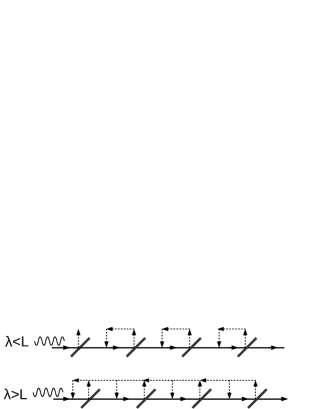
Figure 12: (a) The Brownian wave length within one period is smaller than the length of one local potential well. (b) The Brownian wave length is larger than the length of an unit of potential well.

If the random wave length $\lambda_{Brownian}$ is smaller than $L$, the propagating wave only collide with one beam splitter, or one potential well(Fig. 12). The transmission probability is $p=b/(a+b)$, while the reflection probability is $1-p=a/(a+b)$. Here the definition of transmission and reflection depends on the direction of input wave, one may switch $a$ and $b$ for different cases. If the random wave length $\lambda_{Brownian}$ is larger than $L$, the propagating wave will cover two potential wells at the same time. In that case, the wave will pass two beam splitters within one period. We must sum up all possible path within two-steps, it has been shown in my optical model of Parrondo-Harmer-Abbott game. But here the case is simpler for all the beam splitters are identical. If the random wave length $\lambda_{Brownian}$ is so large that it covers many potential wells at the same time, we must take into account of three or more beam splitters at one time. This case meet the history dependent game with long term memory.

The two or more steps of collision between neighboring potential wells can be mapped into a limited number of elementary optical diagrams. I showed the optical diagram of two steps of collision in Fig. 13. The transmission is in the same direction as the incoming velocity. While the reflection is in the opposite direction. Every reflection bond is labeled by a number, $-(1-p)=e^{i\pi}(1-p)$. If Brownian particle pass two potential wells continuously, we label it as state $\lvert\textbf{11}\rangle$. The final output particle moves in the same direction as the input velocity. The state $\lvert\textbf{10}\rangle$ denotes that the Brownian particle first pass one potential well and then is reflected by the next potential well. The final output velocity of state $\lvert\textbf{10}\rangle$ is in the opposite direction of the input velocity. So does the state $\lvert\textbf{01}\rangle$. For the state $\lvert\textbf{00}\rangle$, the Brownian particle is firstly reflected into the opposite direction at the first potential well, then it is reflected back to the original direction by the second potential well. The final velocity is in the same direction as input velocity. With this correspondence between optical diagram and collision within two neighboring potential wells, one can calculate the final output velocity of Brownian particles in flashing ratchet. Adding up the probability of $\lvert\textbf{00}\rangle$ and $\lvert\textbf{11}\rangle$ gives the positive velocity,

$$V^{+}=P(\lvert\textbf{00}\rangle)+P(\lvert\textbf{11}\rangle).$$ (65)

The negative velocity is determined by $\lvert\textbf{00}\rangle$ and $\lvert\textbf{11}\rangle$,

$$V^{-}=P(\lvert\textbf{01}\rangle)+P(\lvert\textbf{10}\rangle).$$ (66)

If $\lvert V^{+}\rvert>\lvert V^{-}\rvert$, the particle moves in the same direction as its original velocity. On the contrary case, the particle move in the opposite direction. If $\lvert V^{+}\rvert=\lvert V^{-}\rvert$, the particle is trapped in a local potential well and moves around randomly. If the length of unit potential well is much smaller than the phenomenological random wavelength, we must include the three-steps of collision or even more steps. The strategy is the same as I showed above.

Figure 13: The four elementary optical diagrams for a particle propagating through two beam splitters. The right hand side is the corresponding behavior of a Brownian particle colliding with two neighboring potential wells.

If Brownian particles do not collide with each other, the physics of single particle is an ideal meanfield approximation of many particle system. In fact, the random wave length $\lambda_{Brownian}$ is only well defined for a crowd of many Brownian particle. When many Brownian particles are trapped in a periodic potential, the collision between different particles are modulated to form quasi-regular density wave. When this density wave propagates across the periodic potential, it is either reflected or transmitted. Modeling many colliding Brownian particles as density wave is convenient for describing and calculating Brownian rachet in two dimensional periodic potential(Fig. 14 (a)). In two dimensional periodic potential, a Brownian particle can circumvent potential wells instead of being blocked there. If the Brownian particle can randomly fluctuate around a circle, such as sperm or bacteria, the angular velocity is equivalent to an effective magnetic field. In quantum Hall effect of electrons in magnetic field, a series of plateaus appear in the Hall resistance measurement. This give us a hint that the two dimensional flashing rachet for circling Brownian particle maybe has significant different phenomena from one dimension.

$\begin{array}[]{c@{\hspace{0.2in}}c}\vspace{0.1cm}\includegraphics[width=86.72267pt]{twoD.eps}\hfil\hskip 14.45377pt&\includegraphics[width=108.405pt]{convert.eps}\\ \mbox{(a)}\hfil\hskip 14.45377pt&\mbox{(b)}\\ \end{array}$

Figure 14: (a) The asymmetric potential well for Brownian rachet periodically distributed in two dimensions. (b) Elementary flipper and its combination. Each box represents a flipper which corresponds to one losing game. A losing game is operated by odd number of elementary flipper. A winning game can be performed by even number of flipper.

When the local density of Brownian particle oscillates periodically under the modulation of external potential, it may be called as density wave. It is hard to control exactly the local density, but in a game, a player can determine the amount of his capital for each round of game. If we play the capital in a proper way, it will generate a good correspondence between Brownian density wave and capital wave of game.

First, we decompose the input capital as the integration of a pair of conjugated complex function, $N=\int{\psi^{\ast}\psi}=\langle\psi\lvert\psi\rangle$, $\psi_{t}$ is a wave function whose amplitude is the square root of the total capital,

$$\psi=\psi_{a}(t)+i\psi_{b}(t)=\sqrt{N_{t}}\exp[{i\Omega{(t)}}],$$ (67)

The angular velocity $\Omega(t)=\arctan[{\psi_{b}(t)/\psi_{a}(t)}]$ is a complicate function of time. The capital now has internal degree of freedom. Suppose we input capital $1000$ points within time interval $T$. But they do not join the game one after another in constant speed or once and for all. We divide those time interval into $n$ pieces, $T=[0,T_{1})\cup[T_{1},T_{2})\cup[T_{2},T_{3})\cdots\cup[T_{n-1},T_{n}]$. The input capital in each step is $N_{T_{i}}$ which is oscillating within $T$, and $\sum_{i}N_{T_{i}}=1000$. For example, we input an cosin wave, $N=\cos[\Omega{(t)}],\;t\in{T}$. Then $N_{T_{i}}=\int^{T_{i}}_{T_{i-1}}\cos[\Omega{(t)}].$ The discrete capitals within $T$ now are not unrelated numbers, they organized into waves. This give us the real part of the capital wave $Re[\psi]=\sqrt{N}\cos[\Omega{(t)}]$. The imaginary wave of the capital is the delayed or advanced real wave by a phase of $\pi/2$, $Im[\psi]=\sqrt{N}\cos[\Omega{(t)}\pm\pi/2]$. The total input capital is

$$N=Re[\psi]^{2}+Im[\psi]^{2}.$$ (68)

When a beam splitter received the capital $Re[\psi]^{2}$ and $Im[\psi]^{2}$, it take them as independent beams and redistribute them separately. Both the real wave and delayed real wave(or imaginary wave) generate a transmission wave and reflection wave, we sum the transmission up and denote it as $\psi_{\textbf{1}}$. The sum of refection is $\psi_{\textbf{0}}$. The total capital wave if the sum of the two waves, $\psi=\psi_{\textbf{1}}+\psi_{\textbf{0}}$. We use Dirac bracket to express the winning wave as $\lvert{\textbf{1}}\rangle\rightarrow\psi_{\textbf{1}}$, the losing wave is $\lvert{\textbf{0}}\rangle\rightarrow\psi_{\textbf{0}}$, $\lvert{\psi}\rangle=\lvert{\textbf{1}}\rangle+\lvert{\textbf{0}}\rangle.$ Then the absolute value of total capital reads

$$N=\langle{\textbf{1}}\lvert{\textbf{1}}\rangle+\langle{\textbf{0}}\lvert{\textbf{0}}\rangle.$$ (69)

We have assumed there is no overlap between reflection and transmission, thus $\langle{\textbf{0}}\lvert{\textbf{1}}\rangle=\langle{\textbf{1}}\lvert{\textbf{0}}\rangle=0$. $\langle{\textbf{1}}\lvert{\textbf{1}}\rangle=\rho_{11}$ is transmission probability determined by the beam splitter. $\langle{\textbf{0}}\lvert{\textbf{0}}\rangle=\rho_{00}$ is the reflection probability.

If the input angle between capital wave and beam splitter is so small that reflection overlaps transmission, the transformation between reflection and transmission is not zero, i.e., $\langle{\textbf{0}}\lvert{\textbf{1}}\rangle\neq\langle{\textbf{1}}\lvert{\textbf{0}}\rangle\neq 0$. In that case, the total transmission is $N_{\textbf{1}}=\langle{\textbf{1}}\lvert{\textbf{1}}\rangle+\langle{\textbf{1}}\lvert{\textbf{0}}\rangle$. The total reflection is $N_{\textbf{0}}=\langle{\textbf{0}}\lvert{\textbf{0}}\rangle+\langle{\textbf{0}}\lvert{\textbf{1}}\rangle$. The reflected capital must carry a phase factor $e^{i\pi}$,

$$N_{\textbf{0}}=e^{i\pi}[\langle{\textbf{0}}\lvert{\textbf{0}}\rangle+\langle{\textbf{0}}\lvert{\textbf{1}}\rangle].$$ (70)

A winning game requires more transmitted capitals than the reflected ones. The final gain of the game, $G(t)$, is

$$G(t)=N_{\textbf{1}}+N_{\textbf{0}}>0.$$ (71)

In the meantime, the sum of the two absolute values are the total number, $N={\lvert}N_{\textbf{1}}{\lvert}+{\lvert}N_{\textbf{0}}{\lvert}$. We can define normalized transmission $p={\lvert}N_{\textbf{1}}{\lvert}/N$ and normalized reflection $1-p={\lvert}N_{\textbf{2}}{\lvert}/N$ to get rid of the dependence on the absolute value of input. If the gain $G(t)<0$, the game loses.

Any game has an input and output. The output is either win or loss. If we input a positive capital, a positive output corresponds to the win, a negative output corresponds to the lose. If we add a negative sign on the input, the output will flip a sign correspondingly. If the game either transform the positive input capital into a negative output or transform the negative input into positive output, this is always a losing game, we call the game a flipper. A flipper check the sign of input and sent out an output with opposite sign. The simplest flipper is a mirror with total reflection.

Single game consisting of odd number of flipper is losing game, while the combination of even number of flipper is a winning game. For example, we take a sequence of flippers, $\{A,B,C,D,\cdots\}$ (Fig. 14 (b)). The flipper A maps the input capital $C_{in}$ to $C_{out}$ under the constraint $C_{in}{\times}C_{out}=-1$, so do the flippers $\{B,C,D,\cdots\}$. Different flipper produce different ratio between output capital and input capital, we denote this ratio $C_{out}/C_{in}$ as amplification, $F_{\alpha}=C^{\alpha}_{out}/C^{\alpha}_{in}$, here $\{\alpha=A,B,C,\cdots\}$ is the label of the flipper. The amplification of a flipper is always negative, $F_{\alpha}<0$. If we play flipper A, it always lose, any positive capital turns out to be negative. But flipper A also transform negative capital into positive capital. If we play two flipper $A$, the output of the first A is the input of the second A, then the positive input capital at the first A will give out a positive output at the second A. The amplification of the double A game is $F_{AA}=F_{A}F_{A}>0$, $F_{A}<0$. If we play a sequence of flipper $\{A,B,C\}$, the final amplification is $F_{ABC}=F_{A}F_{B}F_{C}<0$. For the most general case, the product of a sequence of flipper, $\{\alpha{i},i=1,2,3,\cdots\}$, the final amplification is

$$F=\prod_{{i}=1}^{n}F_{\alpha{i}}.$$ (72)

If $n=2k+1$, $F<0$, it is losing game. If $n=2k$, $F>0$, it is winning game.

The input and output of any flipper must be classical variables. The player is actually a classical observer. The player make decisions following classic logic. A flipper may have complex internal game process dealing with complex quantum states. When we try to check the output of a flipper to see it wins or loses, we must measure the weight of those states, all the results will be summarized into a classical number. Therefore the inter-junction between independent flippers is always classical operation, no quantum states could survival. Quantum states may be used to design the internal gaming process within a flipper. If two independent flipper are perfectly organized into one combined flipper, then the old interface between single flippers disappeared. The quantum states can flow through those old classical channels. If we cut the united flipper into two parts without measuring the cutting edge, the quantum states are still waiting on the interface. But we can not determine wether each part wins or lose. They will collapse into classical numbers if we perform measurement.

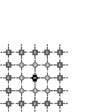
Figure 15: The dark star in the center is where the game begins, input capital is injected there. The box with label 1 represents the direct product of odd number of elementary flippers. The box labeled by 2 represents the direct combination of even number of flippers. The cups attached to the wall represent quantum state collector.

Strictly speaking, there is no quantum game paradox as long as we want a definite output state of either winning or losing for each sub-flipper. Quantum states can be used to design the internal structure of single flipper. For example, we choose electron with spin as player. The winning state is more spin-up than spin down, the losing state is the opposite case. The input electrons may be all spin-ups. Then we design various complex scattering process within the flipper, such as two slits, many slits, magnetic field, electric field, other fixed nuclear spin, and so on. On the output side, we measure the state of all output electron. If the total number of spin-ups is more than those spin down, the game wins, this is not successful flipper. This design must be abandoned and start a new design until we get more spin-down than spin-up. Once we get a flipper with quantum internal structure, and make a good interface between the output of one flipper and the input another flipper, one can play the game paradox using many copies of the same flipper. From a global point of view, this is a classical game. If we go inside every flipper, it is a quantum processor.

A single flipper does not results in so-called game paradox. It is only when we combine many flippers in a complex way, the player can not read out the final output at first sight, the total game will produce seemly strange results. To find out the output of flipper network has a lot of things in common with many body physics. Especially when the flipper are quantum processors, we are essentially manipulating various entangled quantum states from local flipper to reach a global winning output. I showed an example of combinate game on $5\times 5$ square lattice(Fig. 15). This game is the combination of 25 sub-games. There are 14 losing games, and 11 winning games. The winning game are performed by the winning processor which is produced by even number of elementary flippers. They are represented by the boxes labeled by 2. The processor produced by odd number of elementary flipper are in charge of the losing games, they are labeled by 1(Fig. 15). The game starts from the dark star in the center. The dark star is a losing processor, it gives out four outputs. At the next step, the four outputs flow into a ring of eight processors. Three of them wins(the disc with label 2 in Fig. 15) The other five would lose(the disc with label 1 in Fig. 15). The $12$ outputs of this ring provide the input for the last round of game. There are $16$ processors in the last round, $8$ lose and 8 win. The output result at the first round of game can be read out by performing measurement on each of the 12 output. The output states from winning processors are projected to final winning state $\langle\textbf{1}\lvert$, this give the positive gain. While the output of those losing processors counts the negative gain. The total gain is the sum of all the outputs of this round,

$$G(t)=\sum_{i,j,\alpha}\left[\langle\textbf{1}_{d}\lvert\psi_{{}_{d(i,j)}}^{\alpha}\rangle-\langle\textbf{0}_{d}\lvert\psi_{{}_{d(i,j)}}^{\alpha}\rangle\right],$$ (73)

the indexes $i,j$ runs over all the eight processors represented by disc in Fig. 15. If $G(t)>0$, the game wins, otherwise the games loses. For a game combined $n\times{n}$ subgames, the total number of output at the last round of game is $n^{2}+4$. If every sub-game is different from another, the dimension of probability variables is $n^{2}$. However we have only one equation to solve, $G(t)>0$. Even if all the sub-games are losing, the solution space is a $n^{2}$ dimensional cubic, each edge of the cubic has a length of $[0,1/2)$. To solve one inequality equation of $n^{2}$ unknown variables is a trivial problem. But if all the subgames labeled by 1 are the same, so does the game with label 2. We have only two variables which are distributed on the whole lattice, it is an interesting question to ask wether the combined game wins or loses.

To find out the final output of flipper network has a lot of things in common with many body physics. Especially when the flipper are quantum processors, we are essentially manipulating various entangled quantum states from local flipper to reach a global winning output. Many coupled identical flippers on a regular lattice can be theoretically summarized into a many body Hamiltonian system. Each flipper represents one losing game, this many body system represent a complex game of many coupled losing sub-games. We interested in the existence of a winning combined game out of many losing games, or the opposite case. Although this is no longer a paradox due to the strong coupling between neighboring losing games, it is still an interesting question. I will take many Ising spins on square lattice as an example to show how to model a quantum many body system into a combined game of many losing sub-games. We use Pauli matrix $\sigma^{x}_{i}$ to express a flipper. Each flipper occupied one lattice site. The nearest neighboring flippers couple with each other to work together. The output of the flipper pair $\sigma^{x}_{i}\sigma^{x}_{j}$ for the input state $\lvert{s_{i}s_{j}}\rangle$ is

$$h_{ij}=\langle{s_{i}s_{j}}\rvert\sigma^{x}_{i}\sigma^{x}_{j}\lvert{s_{i}s_{j}}\rangle,$$ (74)

$s_{i}=\pm 1$ is Ising spin. The output operator of the combined game on the whole lattice is Hamiltonian

$$H=\sum_{<ij>}J_{ij}\sigma^{x}_{i}\sigma^{x}_{j},$$ (75)

where $<ij>$ denotes the nearest neighboring lattice sites. $J_{ij}$ is the coupling strength. The input capital is the difference between the total number of spin $+1$ and the total number of spin down $-1$ in any given initial state

$$\lvert{\psi_{input}}\rangle=\lvert{s_{1}s_{2}s_{3}\cdots s_{n}}\rangle.$$ (76)

For instance, $\lvert{\psi_{input}}\rangle=\lvert{1,-1,1,\cdots,-1,-1,1,}\rangle$. The game rule is to minimize the total energy to reach a ground state. Playing one round of game is performed by operating the Hamiltonian on the initial configuration once. The output state after $k$ rounds of game is

$$\lvert{\psi^{k}_{output}}\rangle=H^{k}\lvert{\psi_{input}}\rangle.$$ (77)

The spin configuration at each round of game must make sure that the total energy $E=\langle{\psi}\rvert{H}\lvert{\psi}\rangle$ decreases comparing with last round of game. We take $s_{i}=+1$ as the positive capital for the game, if it becomes $-1$ in the end, the game lost. The total game covers many sub-games. If we input less $\{s_{i}=+1\}$, but end up with more $\{s_{i}=+1\}$ than our input, the games wins. The Hamiltonian Eq. (75) is equivalent to the familiar Ising Hamiltonian $H=\sum_{<ij>}J_{ij}\sigma^{z}_{i}\sigma^{z}_{j}$. Theoretical physicist always search for the stable spin configurations of ground state starting from an arbitrary initial configuration, especially in quantum monte Carlo simulations. The so-called game paradox appears almost everywhere in many different quantum models. In mind of the great interest on time series in stochastic dynamics, what quantum Monte Carlo simulation has abandoned during the process of finding ground states maybe can help people to design winning games by combining a large number of lost sub-games. On the other hand, the so-called game paradox remind us that designing different non-equilibrium game process maybe leads to different physical properties of many body system.

VII Summary

When we divide a complex winning game into many sections, each section has an input and output, we call it a sub-game. Every sub-game must be tested to see wether it is a losing or winning game. It is not against intuition that if all sub-games are lost. More over, if we combine these sub-games together but in a different order as the original one, it is not against intuition either if the combined game is a losing game. No mater it is dividing or combining, we are dealing with the correlations between those sub-games. A real game paradox only exist when there is no any correlation between sub-games. In that case, any conclusion about the total game based on the result of sub-games are not reasonable.

Both Parrondo-Harmer-Abbott game and Parrondo’s game introduced the correlation of probabilities between the nearest two rounds of game. In mind of a fact that the first round and the second round are the nearest neighbor, the second round and the third round are also nearest neighbor, and so forth, it forms a long chain of many coupled sub-games in history. In my optical analogy, the photon propagates through a long path connecting many beam splitters. The photon is either reflected or transmitted at each beam splitter. The final intensity of this photon is the product of the reflection or transmission coefficient of every beam splitter along this path. The more rounds of game one played, the more paths one would have. We sum up the intensity of all possible paths to reach the final output. If we have more transmitted photon than reflected photons, the final gain would be positive, the game wins, otherwise the game lost. If the photon is reflected for odd number of times, its contribution to the final gain is negative. If the photon is reflected even number of times, its contribution is positive. Since reflection photon can transmit through or reflected by other beam splitter, the lost of one local sub-game can become positive when a negative photon is reflected again by another beam splitter. Both Parrondo-Harmer-Abbott game and Parrondo’s game can be mapped exactly into the propagation of a photon through the array of beam splitters.

To implement Parrondo-Harmer-Abbott game, we can use the same type of physical beam splitters with different transmission and reflection coefficient. While to implement Parrondo’s old game, we need two different types of beam splitter: one add a $e^{i\pi}$ phase shift to its reflection, the other does not. There is modular operation in Parrondo’s old game that the capital in game must be checked to see if it can be divided by a integer or not. This modular operation is equivalent to a special beam splitter from the point view of probability distribution. If we put this special beam splitter aside and only compare the optical diagram structure of Parrondo-Harmer-Abbott game and Parrondo’s old game, they are essentially same. Parrondo-Harmer-Abbott game and Parrondo’s game simulate the random sequence of combing game A and game B, the final game is winning. In fact, what really matters is the coupling between the two steps in game B, no matter how random the sequence of $ABAABBA\cdots$ are, it does not break the internal coupling inside game B. It is through the coupled two steps, or in other words, through two neighboring beam splitters, the probability of negative capital is transformed into the probability of positive capital. This lies in the heart of a winning combined game out of losing games.

We come to the conclusion: there is no paradox in both Parrondo-Harmer-Abbott game and Parrondo’s old game, these two games are both reasonable and share the same strategy of coupling the nearest two rounds of game. This is a good news to gamblers for they can win from loss by reasonable calculations without worrying about paradox.

One can design much more complex games by drawing optical diagrams following the same strategy I used. A three-step history-dependent game is designed as an example to show how to combine many games. In this game, even if all the sub-games lost, the output of this combined game can win, lose or oscillating between loss and win. Different probability distribution leads to different results. To calculate the final output, one can draw all the paths connecting beam splitters. The final gain of each path is derived by multiplying the value of probability of all the bonds along this path. Summing up all the paths gives the final gain. A real photon propagating across array of beam splitters provide a practical way to test the complex design.

Since correlation can make losing games win, it is a good strategy to implant more correlations among sub-games. I designed a history entangled game with only two sub-games. The input state of each sub-game depends on the symmetric or antisymmetric combination of the historical states two steps earlier. In the symmetric states, two winning sub-games may leads to a lost combined game. If one of them wins, the game can win. In the antisymmetric state, two losing game results in a winning combined game. If one wins, the other lost, the output is either lose or win, it depends on specific parameters. In some parameter region, the final gain oscillates between win and loss.

We can implant strong correlations into the capital instead of sub-games. This is in case if one can not modify the game rule, but one can change the way of playing the capital in hand. Suppose one has $1000$ points in the beginning, we cut it into many pieces, $100+350+10+50+\cdots=1000$. Then we invest the capital in game according to a wave pattern, such as $\cos[t]^{2}+\sin[t+\tau]^{2}$, $\tau$ is the delay time. When this capital wave propagates through the lattice of many coupled sub-games, the outputs of sub-games are strongly entangled. To determine the final output of these quantum entangled states is equivalent to solve a quantum many body physics problem. For example, when we search for the spin configuration of ground state on a lattice, usually it starts from a random initial spin configuration, this initial configuration can be viewed as input capital of a game. Then we update the initial configuration by applying a functional of Hamiltonian operator, this is a process of combined game, every local operator on single lattice is a sub-game. The final output of the game is stable spin configuration. This is how quantum Monte Carlo simulation runs everyday. In fact, Monte Carlo method, as its name suggested, comes from gamble games.

Coupled many sub-games is useful for designing various complex Brownian ratchet. The one dimensional periodic asymmetric potential is equivalent to a chain of many beam splitters. If a flashing Brownian can cover two or more potential well within one period, we must take into account of the coupling between two or more neighboring potential wells. The forward velocity is determined by summing up continuous two steps of pass or refelection. The backward velocity is determined by the joint probability of one reflection followed one pass or vice verse. The optical model provide a tool to analyze the relationship between different individual potential wells. Especially when there are many different individual local potential wells distributed along the long chain. If each local potential well has different reflection and transmission, it is hard to see the physics directly from Fokker-Planck equation or Smoluchowski equation. In that case, we take every local potential well as a different beam splitter, draw the optical diagram, then one will get at least a phenomenological understanding.

VIII Acknowledgment

References

- (1) The I Ching or Book of Changes. Translated by R. Wilhelm, rendered into English by C. F. Baynes, forword by C. G. Jung. Bollingen Series XIX. Princeton University Press, (1950).
- (2) A. Allison and D. Abbott, in Proceedings of the 2 nd International Conference on Unsolved Problems of Noise(UPoN’99) (Ref[6]), Vol. 511, p. 249.
- (3) J. M. R. Parrondo, How to cheat a bad mathematician. EEC HC M Network Workshop on Complexity and Chaos (contract no. ERBCHRX-CT 940546), Turin, Italy (1996).
- (4) G. P. Harmer and D. Abbott, Nature 402, 864 (1999).
- (5) A. Chubukov, Phys. Rev. Lett. 69, 832 (1992).
- (6) J. Villian, R. Bedaux, J. P. Carton, and R. Conte, J. Phys.(Paris), 41, 1263 (1980).
- (7) J. M. R. Parrondo, G. P. Harmer and D. Abbott, Phys. Rev. Lett. 85, 5226 (2000).
- (8) R. J. Kay and N. F. Johnson, Phys. Rev. E 67, 056128 (2003).
- (9) J. Rousselet, L. Salome, A. Ajdari and J. Prost, Nature 370, 446 (1994).