$SU(3)$ Landau gauge gluon and ghost propagators
using the logarithmic lattice gluon field definition

Abstract

We study the Landau gauge gluon and ghost propagators of $SU(3)$ gauge theory, employing the logarithmic definition for the lattice gluon fields and implementing the corresponding form of the Faddeev-Popov matrix. This is necessary in order to consistently compare lattice data for the bare propagators with that of higher-loop numerical stochastic perturbation theory (NSPT). In this paper we provide such a comparison, and introduce what is needed for an efficient lattice study. When comparing our data for the logarithmic definition to that of the standard lattice Landau gauge we clearly see the propagators to be multiplicatively related. The data of the associated ghost-gluon coupling matches up almost completely. For the explored lattice spacings and sizes discretization artifacts, finite-size and Gribov-copy effects are small. At weak coupling and large momentum, the bare propagators and the ghost-gluon coupling are seen to be approached by those of higher-order NSPT.

I Introduction

During the last years lattice studies on the Landau gauge gluon and ghost propagators have clearly Cucchieri and Mendes (2008a, b); Bogolubsky et al. (2009a); Bornyakov et al. (2010) not confirmed the asymptotic infrared behavior as postulated by the Gribov-Zwanziger scenario Gribov (1978); Zwanziger (1994) or required by the Kugo-Ojima confinement criterion Kugo and Ojima (1979). The inconsistency seems to be related to the treatment of the Gribov problem, i.e., the non-uniqueness of the Landau gauge condition in the non-perturbative regime (at least in finite volumes). In our opinion, it is still unclear, whether the lattice formalism—for a fixed gauge—requires a reformulation in order to become consistent with a BRST-invariant continuum theory or whether the continuum approach itself needs to be reformulated (see also Fischer et al. (2007); von Smekal (2008)). We would like to stress that until now no complete gauge-fixing prescription for Landau gauge has been agreed upon (see, e.g., Maas (2010); Maas et al. (2010) and references therein). At the same time it is clear that the gauge-invariant lattice formulation of $SU(N)$ Yang-Mills theories does provide confinement of quarks and gluons. Also in the context of gauge-variant approaches, there are clear signals that quarks and gluons (and ghosts) are not part of the physical spectrum, for example, by the violation of reflection positivity  Cucchieri et al. (2005); Sternbeck et al. (2006); Bowman et al. (2007). The exact mechanism of confinement, however, is still unknown. It should be added though that a direct link between quark confinement, as measured by the Polyakov-loop order parameter, and the infrared behavior of ghost and gluon Green’s functions has been established recently Braun et al. (2010).

However, the infrared asymptotics can only be one aspect. Another, by no means less important, should be the computation of QCD’s elementary two- and three point functions in the intermediate (around $1\mathrm{~{}GeV}$) and ultraviolet momentum region. This would allow for example to determine essential phenomenological parameters, like the QCD scale $\Lambda_{\overline{\mathsf{MS}}}$, or gluon and quark condensates (see, e.g., Becirevic et al. (2000); Boucaud et al. (2006, 2005, 2009); Sternbeck et al. (2009); Blossier et al. (2010)). Moreover, such calculations are important to arrive at renormalized propagators, and eventually also at vertex functions, which, calculated on the lattice and extrapolated to the continuum limit, could serve as input to a Bethe-Salpeter or Faddeev equations based hadron phenomenology (see, e.g., Alkofer et al. (2010) for a status report).

Therefore, the validity of multiplicative renormalizability in the nonperturbative regime as well as the speed of convergence to the continuum limit, and its uniqueness, are essential questions that need to be addressed on the lattice in this context. For the gluon field this has been done in the past Giusti et al. (1998); Petrarca et al. (1999); Furui and Nakajima (1999); Cucchieri and Karsch (2000); Bogolubsky and Mitrjushkin (2002), in particular there with respect to the question of universality of its definition on the lattice. Also, more recently, first steps towards continuum-limit-extrapolated lattice data for the gluon and ghost propagators have been presented Bornyakov et al. (2010); Bogolubsky et al. (2009b).

With our study we intend to provide further input to such projects, placing here particular emphasis on connecting lattice Monte Carlo studies with those of lattice perturbation theory (LPT). Specifically we will confront its numerical variant, the numerical stochastic perturbation theory (NSPT) Di Renzo et al. (2010a); Di Renzo et al. (2011), with lattice Monte Carlo (MC) data of the gluon and ghost propagators and the associated ghost-gluon coupling in Landau gauge von Smekal et al. (1997). This will help to quantify the region where predictions of NSPT are valid.

So far, most MC studies of these gauge-variant objects have used (what we call below) the linear definition

$$A^{\rm(lin)}_{x+\frac{\hat{\mu}}{2},\mu}=\frac{1}{2iag_{0}}\left(U_{x,\mu}-U^{\dagger}_{x,\mu}\right)\Big{|}_{\rm traceless}$$ (1)

with $a$, $g_{0}$ denoting the lattice spacing and the bare coupling, respectively. On the lattice, however, the definition of the gluon field (and also of the Faddeev-Popov operator) is in no way unique. One can of course equally well use another definition, for example, that of the modified lattice Landau gauge von Smekal et al. (2007), or the quadratic definition

$$A^{\rm(quad)}_{x+\frac{\hat{\mu}}{2},\mu}=\frac{1}{4iag_{0}}\left[(U_{x,\mu})^{2}-(U^{\dagger}_{x,\mu})^{2}\right]\Big{|}_{\rm traceless}$$ (2)

which has been studied and compared with the linear definition in Refs. Giusti et al. (1998); Petrarca et al. (1999). It was also shown there both converge towards the same continuum limit.

Yet another definition is known as the logarithmic definition of the lattice gluon field,

$$A^{\rm(log)}_{x+\frac{\hat{\mu}}{2},\mu}=\frac{1}{iag_{0}}\log\left(U_{x,\mu}\right)\,.$$ (3)

This definition has been put forward for lattice MC studies by Furui and Nakajima (see, e.g., Furui and Nakajima (1999); Nakajima and Furui (2000); Furui and Nakajima (2004a, b, 2006)). It is also the definition being used in lattice perturbation theory (see, e.g., the monograph Rothe (1997)) and NSPT. Since we are aiming at a quantitative comparison of NSPT with lattice MC data, below we will mainly concentrate on this definition.

The respective control functional for the Landau gauge, the quadratic norm

$$||\Delta||^{2}=\sum_{x}~{}\operatorname{tr}\Delta(x)\Delta^{\dagger}(x)\,,$$ (4)

is given in terms of the lattice divergence

$$\Delta=\left(\sum_{\mu}\partial_{\mu}A_{\mu}\right)(x)\equiv\sum_{\mu}\left(A_{x+\frac{\hat{\mu}}{2},\mu}-A_{x-\frac{\hat{\mu}}{2},\mu}\right)\neq 0\,,$$ (5)

for each of these definitions.

When expanded in terms of the lattice spacing all these definitions of the gluon field agree at leading order, but differ beyond that (see, e.g., Sternbeck and von Smekal (2010)). It is because of these differences why the corresponding Jacobian factors (Faddeev-Popov determinants) differ in the integration measure and why the respective lattice Landau gauge condition ($||\Delta||^{2}$) cannot be simultaneously satisfied (see, e.g., Giusti et al. (1998); Petrarca et al. (1999) or below). For a consistent setup of Landau gauge on the lattice one therefore has to employ the corresponding lattice expressions for the gauge functional and the Faddeev-Popov operator. These are available in the literature for all above-mentioned approaches. For practical reasons, though, mostly the linear definition has been adopted.

However, in order to assess the genuine non-perturbative effects in the measured two- and three-point functions, it is desirable to have as a reference point an understanding of the perturbative behavior of these functions in higher-order lattice perturbation theory. In recent years such higher-loop results for the lattice gluon and ghost propagators became available using numerical stochastic perturbation theory (NSPT) Di Renzo et al. (2010a); Di Renzo et al. (2011). These results are for individual momenta at a fixed lattice size and are usually obtained for the logarithmic definition. The advantage of NSPT is that the loop-order that can be achieved only depends on the available computational resources. There are no other restrictions. However, if one wants to confront the unrenormalized NSPT results directly with corresponding data from lattice Monte-Carlo (MC) simulations, one cannot expect the convergence of the former to the bare MC data, when different lattice gluon field definitions are employed. Of course, if multiplicative renormalization is in place the bare propagators for the different definitions are related through finite renormalizations, but for a comparison with NSPT this would bring additional uncertainties. For a quantitative comparison it is thus desirable to use the same lattice definition of the respective gluon field and the Faddeev-Popov operator. In addition, lattice NSPT results take the influence of the hypercubic group into account and thus allow for a comparison of the respective propagators at more off-diagonal momenta which are usually excluded by cuts.

We therefore find it worth to complement the existing data for the Landau gauge gluon and ghost propagators by new sets for the logarithmic definition of the lattice gluon fields and the corresponding Faddeev-Popov operator. The bare propagators can then be confronted directly (i.e., without any additional renormalization) to the results from NSPT. We think that this way much more precise information can be obtained on the regime where NSPT holds.

Note that for a renormalization-group invariant, like for example for the ghost-gluon coupling, denoted $\alpha^{\mathsf{MM}}_{s}(q^{2})$ in the minimal MOM scheme von Smekal et al. (2009); Sternbeck et al. (2009), no rescaling of the data would be necessary, when comparing data obtained for different lattice discretization. Data for this coupling, extracted either for the linear or the logarithmic definition, should match up completely, apart from artifacts due to the lattice discretization. This has been argued and, for $SU(2)$, also explicitly shown already in Sternbeck and von Smekal (2010). This coupling thus serves a reasonable object to systematically investigate discretization effects. Below we will further corroborate these findings for the gauge group $SU(3)$ and compare the available data sets to corresponding ones of NSPT.

Altogether, our aim is threefold:

1. To check universality of the employed lattice definitions by comparing MC results obtained for the logarithmic and linear definition. Such a study is not really new, but we do it simultaneously for the gluon and ghost propagator and the associated ghost-gluon coupling. We confirm that, at least in the momentum ranges considered throughout this paper, the propagators are indeed related to each other by multiplicative renormalization, and that these renormalization constants are such that they exactly cancel each other in the coupling as expected.

2. To compare nonperturbative and perturbative lattice results obtained for exactly the same set of parameters. We emphasize that (in this study) we are not intending to fit lattice results in the perturbative range with higher-order perturbation theory as obtained in the continuum by Chetyrkin and Retey (2000); Chetyrkin (2005); von Smekal et al. (2009). This has been the intention in the lattice references Furui and Nakajima (2004a); Becirevic et al. (2000); Boucaud et al. (2006, 2005, 2009); Sternbeck et al. (2009); Blossier et al. (2010). Here we are rather interested to locate the momentum region where predictions of NSPT are still a good approximation to Monte Carlo results.

3. To report in some detail on the realization and performance of the gauge-fixing algorithm required for the logarithmic definition, as well as to assess the importance of the Gribov ambiguity in this setting.

The paper is organized as follows: In Section II we briefly review lattice Landau gauge for the linear and the logarithmic definition of gluon fields. Section III is then devoted to gauge-fixing algorithms, first for $A^{\rm(lin)}_{x+\hat{\mu}/2,\mu}$, and then for $A^{\mathrm{(log)}}_{x+\hat{\mu}/2,\mu}$. For the latter we test three different implementations: an unaccelerated, a Fourier-accelerated and a multigrid-accelerated gauge-fixing algorithm. We will argue that one should preconditioning these by first fixing the gauge field configuration such that $A^{\mathrm{(lin)}}_{x+\hat{\mu}/2,\mu}$ is transversal, before the actual gauge-fixing of $A^{\mathrm{(log)}}_{x+\hat{\mu}/2,\mu}$ starts. A comparison of the three different implementations including their parameters is given at the end of Section III. In Section IV we present expressions for the gluon and ghost propagators for the logarithmic definition. A brief study on the impact of the Gribov ambiguity is also discussed there. Further results are then presented in Section V, where we first compare the gluon and ghost propagators for the logarithmic definition with those for the linear definition, and then discuss lattice discretization and finite-volume effects. We will demonstrate that data for the coupling $\alpha^{\mathsf{MM}}_{s}(q^{2})$ matches up for both definitions without any rescaling. In Section VI we finally confront our MC results for the propagators and the coupling to the recent results from NSPT Di Renzo et al. (2010a); Di Renzo et al. (2011). We will argue that for large $\beta=6/g_{0}^{2}$ and large momenta the MC data must be restricted to the trivial (i.e. real-valued) Polyakov loop sector in order to reach good agreement. In Section VII we will draw our conclusions. A detailed discussion of the multigrid-accelerated gradient algorithm follows in the Appendix.

II Lattice implementations of Landau gauge

On the lattice the fundamental degrees of freedom are the link variables $U_{x,\mu}$, which are elements of the $SU(3)$ gauge group. If one is interested in gauge-variant quantities, like for example the gluon propagator, one has to adopt a definition for the gluon field $A_{x+\hat{\mu}/2,\mu}$ in terms of these links. Above, we mentioned three ways of defining a gluon field on the lattice, the linear and logarithmic definition will be considered below.

II.1 Linear definition of the gluon field

We first recall the linear definition [Eq. (1)]. For this the Landau gauge condition on the lattice (setting the lattice spacing $a=1$),

$$\Delta^{\rm(lin)}(x) = \left(\sum_{\mu}\partial_{\mu}A^{\rm(lin)}_{\mu}\right)(x)$$ (6)

$$\equiv \sum_{\mu}\left(A^{\rm(lin)}_{x+\frac{\hat{\mu}}{2},\mu}-A^{\rm(lin)}_{x-\frac{\hat{\mu}}{2},\mu}\right)=0\,,$$

is realized, if the gauge functional

$$F^{\rm(lin)}_{U}[g]=\frac{1}{4V}\sum_{x,\mu}~{}\left(1-\frac{1}{3}~{}\operatorname{\mathfrak{Re}}\operatorname{tr}~{}{}^{g}U_{x,\mu}\right)$$ (7)

is in a (local) minimum for a given gauge-fixed configuration

$${}^{g}U^{\hphantom{\dagger}}_{x,\mu}=g^{\hphantom{\dagger}}_{x}U^{\hphantom{\dagger}}_{x,\mu}g^{\dagger}_{x+\hat{\mu}}\,.$$ (8)

Here, $g_{x}\in SU(3)$ is the gauge transformation field that - finally - should put the unfixed gauge field $U_{x,\mu}$ to Landau gauge. As there are many local minima (“Gribov copies”) we assume that unique gauge fixing is achieved by searching for the global minimum for each configuration $U$. In practice, one can only try to get as close as possible to the global extremum. We call this general prescription “minimal Landau gauge”. The minimization of $F^{\rm(lin)}_{U}[g]$ can be accomplished by an overrelaxation algorithm or a combination of a simulated annealing and overrelaxation (see below). This allows to fulfil the Landau gauge condition (6) with the required local numerical precision.

II.2 Logarithmic definition of the gluon field

In the continuum, Landau gauge can also be formulated as a minimization problem of the functional

$$F^{\rm(cont)}_{A}[g]=\frac{1}{N_{c}}\sum_{\mu}~{}\int d^{4}x~{}\operatorname{tr}\left[{}^{g}\!A_{\mu}(x)~{}{}^{g}\!A_{\mu}(x)\right]$$ (9)

with respect to $g(x)\in SU(3)$ acting on $A_{\mu}(x)$ according to

$${}^{g}\!A_{\mu}(x)=g(x)A_{\mu}(x)g^{\dagger}(x)+\frac{i}{g_{0}}~{}g(x)~{}\partial_{\mu}g^{\dagger}(x)\,.$$ (10)

The direct transcription of the continuum extremization problem to the lattice leads to the minimization of a lattice gauge functional

$$F^{\rm(log)}_{U}[g]=\frac{1}{4VN_{c}}\sum_{x,\mu}~{}\operatorname{tr}\left[{}^{g}\!A^{\rm(log)}_{x+\frac{\hat{\mu}}{2},\mu}{}^{g}\!A^{\rm(log)}_{x+\frac{\hat{\mu}}{2},\mu}\right]$$ (11)

for the logarithmic definition of the lattice gluon field [Eq. (3)]. The violation of transversality then can always be checked by computing the divergence

$$\Delta^{\rm(log)}(x) = \left(\sum_{\mu}\partial_{\mu}A^{\rm(log)}_{\mu}\right)(x)i$$ (12)

$$\equiv \sum_{\mu}\left(A^{\rm(log)}_{x+\frac{\hat{\mu}}{2},\mu}-A^{\rm(log)}_{x-\frac{\hat{\mu}}{2},\mu}\right)\neq 0\,.$$

Note that the logarithmic definition requires a diagonalization of the neighboring $SU(3)$ link matrices each time the divergence (12) is evaluated.

We will see that the two lattice Landau gauge conditions [Eqs.(6) and (12)] – if imposed on an arbitrary gauge field configuration – will result in rather different gauge-fixed fields. However, the gluon propagators calculated from the respective gluon fields, i.e, $A^{\rm(log)}_{x+\hat{\mu}/2,\mu}$ or $A^{\rm(lin)}_{x+\hat{\mu}/2,\mu}$, will be seen to be related to each other approximately by a finite multiplicative renormalization. Note also that the gluon fields transformed into momentum space will be transversal, $q_{\mu}\tilde{A}_{\mu}(q)=0$, only if the gauge-fixing procedure fits to the respective definition of $A_{x+\hat{\mu}/2,\mu}$.

III Landau gauge fixing: different algorithms are required

III.1 Linear definition

The linear form of the gauge functional in Eq. (7) suggests to use a relaxation method for its minimization (Los Alamos type gauge-fixing): at given lattice site $x$ the gauge transformation field $g_{x}$ is replaced by $g^{\prime}_{x}$ such that the expression

$$\operatorname{\mathfrak{Re}}\operatorname{tr}\left\{g^{\prime}_{x}~{}W_{x}\right\}$$ (13)

is maximized for a given $W_{x}$, where

$$W_{x}\equiv\sum_{\mu}\left(U_{x,\mu}~{}g^{\dagger}_{x+\hat{\mu}}+U^{\dagger}_{x-\hat{\mu},\mu}~{}g^{\dagger}_{x-\hat{\mu}}\right)$$

This is also known as a “projection onto $SU(3)$”

$$g^{\prime}_{x}\equiv{\rm Proj}_{SU(3)}~{}W_{x}^{\dagger}\,.$$ (14)

For $SU(3)$ $g^{\prime}_{x}$ is typically found using the Cabibbo-Marinari decomposition Cabibbo and Marinari (1982), such that the local $SU(3)$ update of $g_{x}$ proceeds via three successive $SU(2)$ updates. Formally, the update can be viewed as the replacement

$$g_{x}\to g^{\prime}_{x}\equiv r_{x}~{}g_{x}\mbox{~{}~{}with~{}~{}}r_{x}=g^{\prime}_{x}~{}g^{\dagger}_{x}\,.$$ (15)

The speed of convergence is usually improved by replacing the relaxation steps by overrelaxation (OR) steps,

$$g_{x}\to r_{x}^{\omega}~{}g_{x}\,.$$ (16)

The overrelaxation parameter $\omega$ has to be optimized in the interval $1<\omega<2$. The required power of the update matrix $r_{x}$ is approximated via the truncated series

$$r^{\omega}_{x}=\sum_{n=0}^{N}~{}\frac{\gamma_{n}(\omega)}{n~{}!}~{}\left(r_{x}-1\right)^{n}\,,$$ (17)

where $N=3$ or 4, and

$$\gamma_{n}(\omega)=\frac{\Gamma(\omega+1)}{\Gamma(\omega+1-n)}\,.$$ (18)

In order to check the Gribov ambiguity, the OR procedure can be repeated for a number of initial random gauges $g^{(i)}_{\rm initial},~{}i=1,\dots,N_{\rm{copy}}$ typically resulting in different final gauge transformations $g^{(i)}_{\rm final}$ for a given lattice gauge field $U$. The different gauge-transformed fields are known as “gauge copies”. They lead to a corresponding distribution of gauge-functional values $F^{(i)}=F^{\mathrm{(lin)}}_{U}[g^{(i)}]$ (the set of local minima) instead of a unique, but usually unknown absolute minimum.

To shift the distribution of $F^{(i)}$ to smaller values, the initial random gauge transformation can be replaced by one obtained using a simulated annealing algorithm (SA) for gauge-fixing. SA is a Markov chain MC process simulating a Gibbs measure of the form

$$P_{U,T_{g}}[g]~{}\propto~{}\exp\left(-\frac{F^{\rm(lin)}_{U}[g]}{T_{g}}\right)$$ (19)

for the field of gauge transformations $g$, where the gauge temperature $T_{g}$ is lowered step by step after one or a few Markov steps according to some protocol (“SA schedule”) such that the process never passes through real equilibrium states. To our knowledge, the method has been very successfully applied for the first time fixing to maximally Abelian gauge in Bali et al. (1996).

It turned out that with respect to computer time as well as with respect to finding smaller $F^{(i)}$, repeating a combined SA+OR algorithm is more efficient, than repeating the OR algorithm with initial random gauge transformation (see Schemel (2006); Bogolubsky et al. (2007)). For the results presented below we have employed the SA+OR algorithm to gauge-fixing the fields $A^{\mathrm{(lin)}}$ [Eq. (1)] but also to precondition the gauge-fixing of $A^{\mathrm{(log)}}$ [Eq. (3)] (for details see below).

For the SA algorithm we have changed the gauge temperature $T_{g}(i_{s})$ for every new MC sweep ($i_{s}$) according to the SA schedule

$$T_{g}(i_{s})=\left[(T_{g,\min}^{5}-T_{g,\max}^{5})~{}\frac{i_{s}-1}{N_{\rm iter}-1}+T_{g,\max}^{5}\right]^{\frac{1}{5}}$$ (20)

proposed in Schemel (2006) with a restriction to $N_{\rm iter}=3500$ iterations. We have used the initial maximal gauge temperature value $T_{g,\max}=0.45$ and the final minimal value $T_{g,\min}=0.01$.

III.2 Logarithmic definition

For the logarithmic definition of the gluon field (for brevity we call the corresponding algorithm logarithmic gauge fixing), the starting point is the local divergence Eq. (12) evaluated at all lattice sites $x$. The gauge transformations $g_{x}$ (at a given lattice site $x$) is updated locally by $g_{x}\to r_{x}g_{x}$ where $r_{x}$ is the exponentiated local divergence of ${}^{g}A_{\mu}$ evaluated at $x$ according to [Eq. (12)], i.e.,

$$r_{x}=\exp\left(-i\alpha~{}(\sum_{\mu}\partial_{\mu}{}^{g}\!A^{\rm(log)}_{\mu})(x)\right)\,.$$ (21)

The step size $\alpha$ has to be tuned. We call this method the local unaccelerated steepest gradient algorithm (the original “Cornell type” gauge fixing discussed in Ref. Davies et al. (1988)).

It is well-known that this update suffers from critical slowing down which can be ameliorated using a Fourier-accelerated version Davies et al. (1988): at each lattice site $g_{x}\to r_{x}g_{x}$ using

$$r_{x}=\exp\left(-i\alpha\hat{F}^{-1}\left[\frac{q_{\rm max}^{2}}{q^{2}}\hat{F}\left[(\sum_{\mu}\partial_{\mu}{}^{g}\!A^{\rm(log)}_{\mu})(x)\right]\right]\right),$$ (22)

instead. Here $\hat{F}$ denotes the Fourier transformation from the space-time lattice to the 4-momentum lattice and $\hat{F}^{-1}$ the reverse transformation, respectively (for $q^{2}$ see (29) and (30)). One recognizes a sort of smearing of the divergence with the inverse Laplacian. We notice that Furui and Nakajima Nakajima et al. (2001) have also used a non-local algorithm in the form of a Newton-Raphson-type construction of $r_{x}$ using the non-vanishing divergence as a source and the inverse Hessian (Faddeev-Popov operator, expanded in $A_{\mu}$ to some finite order) in place of the inverse Laplacian.

Fast Fourier transformations are less efficient if the lattice is fully parallelized. This could become a problem for large lattices. We circumvented this problem by using the multigrid-accelerated steepest gradient algorithm Goodman and Sokal (1986). In fact, the last expression for $r_{x}$ can be written as

$$r_{x}=\exp\left(-i\alpha\,q_{\rm max}^{2}~{}\Delta^{-1}(\sum_{\mu}\partial_{\mu}{}^{g}\!A^{\rm(log)}_{\mu})(x)\right).$$ (23)

The inversion of the Laplacian on an arbitrary source is a standard problem for a multigrid algorithm. Details on our implementation of the multigrid-accelerated gradient algorithm are given in the Appendix.

We faced the problem that the logarithmic gauge fixing fails to finish successfully for 10% to 50% of all attempts, when starting from a random gauge transformation. The exact failure rate depends on the gauge-fixing method, and grows with the lattice size. A similar problem only rarely occurs in case of the linear gauge fixing using the standard OR algorithm. We found, however, that the logarithmic algorithm works successfully in 99% of the cases if the divergence [Eq. (12)] is already sufficiently small at the start. This can be achieved by preconditioning the logarithmic by a linear gauge fixing. The remaining 1% of cases is dealt with by just repeating the gauge fixing.

     

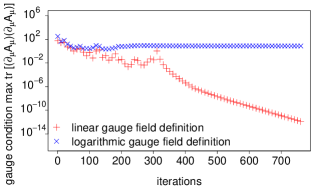
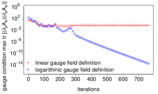
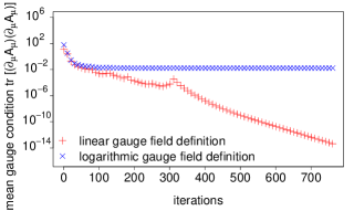
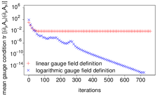
Figure 1: History of maximal values of the squared divergence of the two gluon field definitions during gauge fixing by overrelaxation (left) and the Fourier-accelerated gradient method (right). Example configuration on a $16^{4}$ lattice at $\beta=6.0$.

Figure 2: Same as in Fig. 2 but for the space-time average of the squared divergence of the respective $A_{\mu}$.

III.3 Comparing the two gauge fixing prescriptions

For both types of gauge fixing a stopping criterion is needed. This criterion is fulfilled as soon as the respective divergence, $\left(\partial_{\mu}{}^{g}\!A^{\rm(lin)}_{\mu}\right)(x)$ or $\left(\partial_{\mu}{}^{g}\!A^{\rm(log)}_{\mu}\right)(x)$ is sufficiently small. We have applied the criterion

$$\max_{x}~{}\operatorname{tr}~{}\left[\left(\partial_{\mu}{}^{g}\!A_{\mu}\right)^{\dagger}(x)\left(\partial_{\mu}{}^{g}\!A_{\mu}\right)(x)\right]<10^{-14}\,.$$ (24)

To demonstrate the relation between the two different gauge-fixing algorithms we compare now the history of the overrelaxation and of the Fourier-accelerated gradient algorithm. Both are applied to the same configuration on a $16^{4}$ lattice (generated using the Wilson plaquette action at $\beta=6.0$).

We used $\omega=1.68$ and $N=3$ [see Eq. (17)] for the linear gauge-fixing method (in this case the OR algorithm without the SA-preconditioning step) and $\alpha=0.07$ [Eq. (22)] for the logarithmic gauge fixing (i.e., the Fourier-accelerated gradient algorithm).

In Fig. 2 we compare how the local maxima of the squared divergence of $A^{\rm(lin)}$ and $A^{\rm(log)}$ behave while either the overrelaxation (left panel) or Fourier-accelerated gradient algorithm (right panel) proceeds. When the OR algorithm fixes the Landau-gauge the divergence of $A^{\rm(lin)}$ is successively reduced. This cannot be simultaneously achieved by $A^{\rm(log)}$. On the other hand, when the gradient algorithm fixes the Landau-gauge the divergence of $A^{\rm(log)}$ becomes smaller with every iteration, while the divergence of $A^{\rm(lin)}$ stays almost unchanged. We notice that the local maximum of the squared divergence of the “wrong gauge field” never becomes less than ${\cal O}(1)$. This is the result of only few isolated defects, as it can be seen by a comparison with the corresponding space-time averaged quantities (Fig. 2). The space-time average defined through $||\Delta||^{2}$ [Eq. (4)] reaches a precision of $10^{-4}$, typically after ${\cal O}(100)$ or ${\cal O}(200)$ iterations. To reach the same precision for all lattice sites more iterations are needed. We notice that the space-time average of the squared divergence of the “wrong gauge field” never becomes less than ${\cal O}(10^{-2})$. Comparing the linear and the quadratic definition of the gluon field the authors of Refs. Giusti et al. (1998); Petrarca et al. (1999) have observed a similar difference of $||\Delta^{\rm(quad)}||^{2}$ and $||\Delta^{\rm(lin)}||^{2}$.

Local operators constructed in terms of the gauge-fixed gluon fields can only be sufficiently precise if the respective gauge-fixing method has been used for each $A_{\mu}$. However, as a preconditioner we can (and we do) use the linear gauge-fixing (via the SA+OR algorithm) before applying logarithmic gauge fixing. As mentioned above, this helps much to reduce the number of unsuccessful gauge-fixing attempt for the latter. For the linear definition the SA+OR algorithm always converges.

Preconditioning is not without effect on the final gauge fixing, however. The quality of gauge fixing achieved by the (linear) preconditioner influences the quality of the final (logarithmic) gauge fixing. This is illustrated in Figs. 4 and 4 at $\beta=6.0$ for a $16^{4}$ and $32^{4}$ lattice, respectively.

     

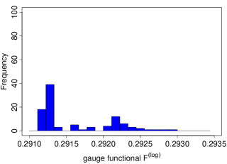
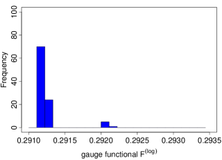
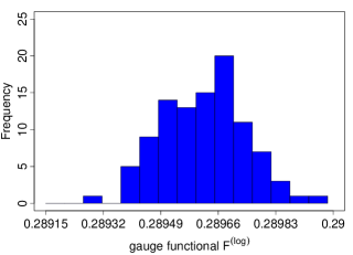
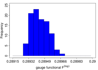
Figure 3: The effect of replacing OR (left) by SA+OR (right) as preconditioner. The figure shows a histogram of final $F^{\rm(log)}$ values for 100 gauge-fixed copies ($16^{4}$ lattice, $\beta=6.0$). The multigrid-accelerated gradient method was used for the gauge-fixing.

Figure 4: Same as Fig. 4, but for a $32^{4}$ lattice.

These figures show the effect of replacing pure OR by SA+OR (with respect to $A^{\rm(lin)}$) as preconditioner for the logarithmic gauge fixing (performed with the multigrid-accelerated gradient method) on the distribution of the final gauge functional values $F^{\rm(log)}_{U}[g^{(i)}]$. This comparison is again for a $16^{4}$ lattice at $\beta=6.0$.

As well-known for the linear gauge fixing, we typically find smaller gauge-functional values also for the logarithmic case, when the SA+OR algorithm is used instead of the OR algorithm for this preconditioning step. This becomes even more pronounced increasing the lattice size where the number of local minima naturally increases.

III.4 Performance of different realizations of the logarithmic gauge fixing

We compare now the logarithmic gauge fixing (without SA+OR preconditioning) in three versions: the unaccelerated gradient algorithm, the Fourier-accelerated gradient algorithm and the multigrid-accelerated gradient algorithm. The advantage of the latter is that it is easy parallelizable. Our code employes a further developed version of the algorithm used by Cucchieri and Mendes for Landau gauge in $SU(2)$ gauge theory Cucchieri and Mendes (1998). In the Appendix our implementation of the multigrid-accelerated gradient algorithm is described in more detail.

  

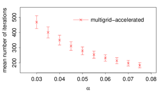
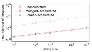
Figure 5: The number of iterations needed to reach the stopping criterion. Left: as a function of the step size parameter $\alpha$ of the multigrid-accelerated algorithm (lattice size $16^{4}$, $\beta=6.0$). Right: as a function of the lattice size for the three investigated logarithmic gauge fixing algorithms ($\beta=6.0$).

In Fig. 5 (left) we show the average number of iterations of the multigrid-accelerated algorithm as a function of the step size parameter $\alpha$ (again for a $16^{4}$ lattices with $\beta=6.0$). With increasing $\alpha$ the mean number of iterations decreases monotonously until it reaches an optimal value $\alpha=\alpha_{\mathrm{opt}}$. Further increasing $\alpha$ beyond that value leads to instabilities and is therefore avoided. In Table 1 we summarize our values on $\alpha_{\mathrm{opt}}$, for the three algorithms and different lattice sizes and $\beta$. Due to limited computing resources, for the bigger lattices we could afford to fix the gauge only by means of the multigrid-accelerated gradient algorithm (in its parallelized version).

Table 1: Optimal values $\alpha_{\text{opt}}$ for the three different logarithmic gauge-fixing algorithms for $\beta=6.0$ and 9.0, and different lattice sizes. Due to the high demand of computation time, $\alpha_{\text{opt}}$ has not been determined for the unaccelerated and the Fourier-accelerated algorithm on lattices larger than $16^{4}$.

algorithm	$\beta$	$8^{4}$	$12^{4}$	$16^{4}$	$24^{4}$	$32^{4}$
unaccelerated	$6.0$	$0.130$	$0.130$	$0.110$	-	-
Fourier-accelerated	$6.0$	$0.070$	$0.070$	$0.070$	-	-
multigrid-accelerated	$6.0$	$0.070$	$0.070$	$0.075$	$0.70$	$0.70$
unaccelerated	$9.0$	$0.125$	$0.125$	$0.125$	-	-
Fourier-accelerated	$9.0$	$0.065$	$0.065$	$0.065$	-	-
multigrid-accelerated	$9.0$	$0.065$	$0.065$	$0.075$	-	-

Fig. 5 (right) presents the scaling of the average iteration number with the lattice size for the three logarithmic gauge-fixing algorithms with their respective $\alpha_{\text{opt}}$ (again all for $\beta=6.0$). We find that these numbers to scale like

$$N_{\rm iter}=C~{}V^{z}\,.$$ (25)

Values for $C$ and $z$ are summarized in Table 2.

Apparently, the two accelerated algorithms perform much better compared to the unaccelerated one, which is mainly due to a much smaller $C$ [compare $\mathcal{O}(10)$ versus $\mathcal{O}(100)$]. The values for $z$ are almost the same for all the three algorithms. We favor the multigrid gauge-fixing algorithm because it is easy to parallelize.

Table 2: The exponent and coefficient, $z$ and $C$, of Eq. (25) for the three different logarithmic gauge-fixing algorithms.

algorithm	C	z
unaccelerated	$110$	$0.33(4)$
Fourier-accelerated	$13$	$0.3(4)$
multigrid-accelerated	$11$	$0.3(4)$

IV Gluon and ghost propagators for $A_{\mu}^{\rm(lin)}$ and $A_{\mu}^{\rm(log)}$

IV.1 Gluon propagator

We are interested in the gluon and ghost propagators for the linear and logarithmic definition. With the lattice gluon field $A^{\rm(lin)}$ and $A^{\rm(log)}$, respectively, the bare gluon propagator is defined as

$$D^{ab}_{\mu,\nu}(x,y)=\left\langle A^{a}_{x+\frac{\hat{\mu}}{2},\mu}A^{b}_{y+\frac{\hat{\nu}}{2},\nu}\right\rangle_{U},$$ (26)

where ${\langle...\rangle}_{U}$ denotes the ensemble average over gauge-fixed configurations. As in most of the applications we evaluate it within the lattice Fourier representation

$$\tilde{D}^{ab}_{\mu\nu}(q(k))=\frac{1}{V}~{}\left\langle\tilde{A}^{a}_{\mu}(k)~{}\tilde{A}^{b}_{\nu}(-k)\right\rangle_{U}$$ (27)

with

$$\tilde{A}^{a}_{\mu}(k)=\sum_{x}~{}A^{a}_{x+\frac{\hat{\mu}}{2},\mu}{\rm e}^{ik\cdot(x+\frac{\hat{\mu}}{2})}\,,$$ (28)

where the abbreviation $k\cdot x=\sum_{\mu}\frac{2\pi k_{\mu}x_{\mu}}{L_{\mu}}$ has been used. $L_{\mu}$ denotes the lattice size in $\mu$-direction. The integers $k_{\mu}\in(-L_{\mu}/2,+L_{\mu}/2]$ count the momentum modes within the Brillouin zone. The lattice momenta can be written in two forms,

$$\overline{q}_{\mu}(k)=\frac{2\pi k_{\mu}}{aL_{\mu}}$$ (29)

and

$$q_{\mu}(k)=\frac{2}{a}\sin\frac{\pi k_{\mu}}{L_{\mu}}=\frac{2}{a}\sin\frac{a\overline{q}_{\mu}}{2}\,.$$ (30)

The latter is the one that appears in the lattice tree-level expression for the gluon propagator, and therefore taken as the corresponding physical momentum.

For the lattice spacing dependence $a(\beta)$ we adopt Necco and Sommer (2002) and use $r_{0}=0.5$ fm to assign physical units to $a$. Table 3 lists the lattice spacing values used in this study.

Table 3: Values for the lattice spacing $a(\beta)$ and its inverse as used in this study. We used the formula given in Necco and Sommer (2002) with $r_{0}=0.5\mathrm{~{}fm}$.

$\beta$	$a(\beta)$ in fm	$a^{-1}(\beta)$ in GeV
$5.8$	$0.1364$	$1.4464$
$6.0$	$0.0932$	$2.1184$
$6.2$	$0.0677$	$2.9137$
$6.4$	$0.0513$	$3.8445$

Supposed all non-diagonal components in the color ($a,b$) and the Euclidean indices ($\mu,\nu$) vanish, one can average $\tilde{D}^{ab}_{\mu\nu}$ over the diagonal elements

$$D(q^{2})\equiv\frac{1}{8}\sum_{a}\frac{1}{3}\sum_{\mu}\tilde{D}^{aa}_{\mu\mu}(q(k))\,.$$ (31)

The factor $1/3$ is due to the transversality of the gluon field with respect to the vector $q_{\mu}(k)$ that leaves only three independent modes. The gluon dressing function is

$$Z_{Gl}(q^{2})=q^{2}D(q^{2})\,.$$ (32)

IV.2 Ghost propagator

For the ghost propagator the situation is somewhat different. It is the two-point function of the ghost fields $c^{a}$ and $\overline{c}^{b}$, and these fields are only implicitly defined through the Faddeev-Popov operator $M^{ab}_{xy}$. Therefore, the bare ghost propagator is defined as the ensemble average of the inverse Faddeev-Popov operator, i.e.,

$$G^{ab}(x,y)=\langle c^{a}(x)~{}\overline{c}^{b}(y)\rangle=\left\langle\left(M^{-1}\right)^{ab}_{xy}\right\rangle_{U}\,.$$ (33)

As mentioned the form of the Faddeev-Popov operator depends on the definition adopted for the gluon field. Generally, on the lattice one can decompose the Faddeev-Popov operator as follows:

$$M^{ab}_{xy}=A^{ab}_{x}~{}\delta_{xy}-\sum_{\mu}\left(B^{ab}_{x,\mu}~{}\delta_{x+\hat{\mu},y}+C^{ab}_{x,\mu}~{}\delta_{x-\hat{\mu},y}\right)\,.$$ (34)

For the linearly defined gluon fields one determines the Faddeev-Popov operator as the Hessian of the gauge functional $F^{\rm(lin)}$ with respect to infinitesimal gauge transformations. This leads to the following form of the adjoint representation matrices entering (34)

$$A^{ab}_{x} = \operatorname{\mathfrak{Re}}\operatorname{tr}\left[\{T^{a},T^{b}\}\sum_{\mu}\left(U_{x,\mu}+U_{x-\hat{\mu},\mu}\right)\right]\,,$$

$$B^{ab}_{x,\mu} = 2~{}\operatorname{\mathfrak{Re}}\operatorname{tr}\left[T^{b}~{}T^{a}~{}U_{x,\mu}\right]\,,$$ (35)

$$C^{ab}_{x,\mu} = 2~{}\operatorname{\mathfrak{Re}}\operatorname{tr}\left[T^{a}~{}T^{b}~{}U_{x-\hat{\mu},\mu}\right]\,,$$

where $T^{a}$ ($a=1,\ldots,8$) denote the generators of $SU(3)$.

For the logarithmic definition the following form of the adjoint representation matrices is used,

$$A^{ab}_{x} = \sum_{\mu}\left[\Omega^{ab}_{x-\hat{\mu},\mu}+\Omega^{ab}_{x,\mu}-A^{c}_{x+\frac{\hat{\mu}}{2},\mu}~{}f^{abc}\right]\,,$$

$$B^{ab}_{x,\mu} = \Omega^{ab}_{x,\mu}\,,$$ (36)

$$C^{ab}_{x,\mu} = \Omega^{ab}_{x-\hat{\mu},\mu}-A^{c}_{x-\frac{\hat{\mu}}{2},\mu}~{}f^{abc}\,,$$

where (written up to fourth order in the gluon field)

$$\Omega^{ab}_{x,\mu} = \Biggl{(}\frac{i~{}A_{x+\frac{\hat{\mu}}{2},\mu}}{1-U^{\dagger}_{x,\mu}}\Biggr{)}^{ab}$$

$$\approx \delta^{ab}+\frac{i}{2}~{}A^{ab}_{x+\frac{\hat{\mu}}{2},\mu}-$$

$$-\frac{1}{12}~{}\left(A^{2}_{x+\frac{\hat{\mu}}{2},\mu}\right)^{ab}-\frac{1}{720}~{}\left(A^{4}_{x+\frac{\hat{\mu}}{2},\mu}\right)^{ab}$$

with the gluon field $A^{ab}$, its square $\left(A^{2}\right)^{ab}$ etc. taken in the adjoint representation.

The Faddeev-Popov operator is inverted with a Laplacian-preconditioned conjugate gradient algorithm and a color-diagonal plane wave source as explained in Sternbeck et al. (2005).

For both the linear [Eq. (IV.2)] and the logarithmic definition [Eq. (IV.2)] the ghost propagator in the momentum space is given by [$q=q(k)$]

$$G^{ab}(q^{2})=\frac{1}{V}\sum_{x,y}\left\langle{\rm e}^{-2\pi i\,k\cdot(x-y)}[M^{-1}]^{ab}_{xy}\right\rangle_{U}=\delta^{ab}G(q^{2})\,.$$ (38)

The corresponding ghost dressing function is

$$Z_{Gh}(q^{2})=q^{2}G(q^{2})\,.$$ (39)

  

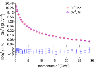
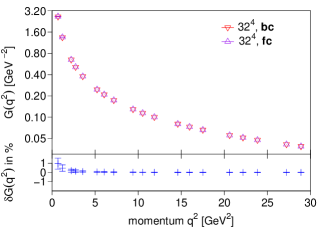
Figure 6: Left: the bare gluon propagator $D(q^{2})$ from the logarithmic gluon field definition and the relative difference $\delta D(q^{2})$ in percent between $\mathbf{fc}$- and $\mathbf{bc}$-configurations generated at $\beta=6.0$ for lattice size $32^{4}$. Right: the corresponding bare ghost propagator $G(q^{2})$ with its relative difference $\delta G(q^{2})$.

IV.3 Momentum cuts

On the lattice, the $O(4)$-symmetry of the continuum Euclidean space-time is broken to the discrete $H(4)$-symmetry. In order to minimize the resulting artifacts, due to the finite lattice volume and spacing we apply two momentum cuts: a cone and a cylinder cut Leinweber et al. (1999).  The cone cut removes all (low) lattice momenta $k=(k_{1},k_{2},k_{3},k_{4})$ with at least one vanishing $k_{i}$. It is applied to minimize finite-volume effects associated with these lattice momenta. The cylinder cut removes all momenta which are not close to a multiple of one of the space-time diagonal unit vectors $n=(1/2)(\pm 1,\pm 1,\pm 1,\pm 1)$. For a symmetric lattice, this criterion can be formulated as

$$\sum^{4}_{i=1}k^{2}_{i}-\left[\sum^{4}_{i=1}k_{i}n_{i}\right]^{2}\leq 1\;.$$ (40)

These two cuts removed most of the lattice artifacts from the data. The remaining artifacts can be assessed using different lattice spacings $a$ and lattice volumes $V$.

IV.4 Gribov ambiguity for $A_{\mu}^{\rm(log)}$-propagators

In order to carry out a first check of the Gribov ambiguity of the gluon and ghost propagators for the logarithmic definition $A_{\mu}^{\rm(log)}$ we used $100$ ($30$) configurations for a $16^{4}$ ($32^{4}$) lattice (again all for $\beta=6.0$). For the larger lattice we expect a stronger influence of the actual selection among the gauge-fixed copies.

Employing the SA+OR preconditioned, multigrid-accelerated gradient algorithm we fix the gauge for each configuration $10$ times starting from different random initializations of the gauge transformation field $g_{x}$. As in Bakeev et al. (2004) for each configuration we have calculated the gluon- and ghost propagator for the first (random) gauge-fixing attempt (first copy, $\mathbf{fc}$) and for the gauge field with the lowest gauge functional value achieved (best copy, $\mathbf{bc}$). Fig. 6 shows the gluon propagator $D(q^{2})$ and the ghost propagator $G(q^{2})$, respectively, averaged over the first and best copies, respectively. In the lower panels of the figures we present also the corresponding relative differences $\delta D$ and $\delta G\equiv$ “($(\mathbf{fc}-\mathbf{bc})/\mathbf{bc}$)” of $\mathbf{fc}$- and $\mathbf{bc}$-results given in percent.

The gluon propagator does not show any effect of the Gribov ambiguity beyond statistical noise (“Gribov noise”) over the whole momentum range, while the ghost propagator seems to exhibit a slight systematic shift within the low momentum region. This shift is approximately $1\%$ for the $32^{4}$ lattice while for the $16^{4}$ lattice it turns out to be negligible. The small effect of the Gribov ambiguity is certainly a consequence of the preconditioning step for which the SA+OR algorithm has been employed. Whether it becomes more enhanced, when taking global $Z(3)$-flip transformations into account Bogolubsky et al. (2008); Bornyakov et al. (2009, 2010), remains to be seen.

In the following we will always rely on $\mathbf{bc}$-results.

V Monte Carlo results for the propagators

V.1 Comparing propagator results for $A_{\mu}^{\rm(lin)}$ and $A_{\mu}^{\rm(log)}$

To get better insight into discretization effects we compare now the gluon and ghost dressing functions for the logarithmic and linear definition. Unfortunately though, we have to restrict the discussion to relatively small lattice sizes.

Table 4: Statistics of Monte Carlo ensembles. $N_{\mathrm{conf}}$ gives the number of analyzed configurations and $N_{\mathrm{copy}}$ of inspected gauge-copies for each. Values are the same for all $\beta$.

lattice	$N_{\mathrm{conf}}$	$N_{\mathrm{copy}}$
$12^{4}$	200	10
$16^{4}$	100	10
$24^{4}$	50	10
$32^{4}$	30	10

The data presented are based on ensembles of gauge field configurations with statistics as given in Table 4.

We consider first the gluon dressing function calculated for the linear and logarithmic definition on a $12^{4}$ and $16^{4}$ lattice at $\beta=6.0$ and $\beta=9.0$. Note that the latter was chosen only in order to compare with available NSPT results (see Section VI). Fig. 7 shows the data for the bare dressing function versus the lattice momentum squared. We clearly see the expected momentum-independent offset between the results for the logarithmic and the linear definition.

  

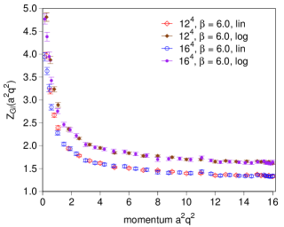
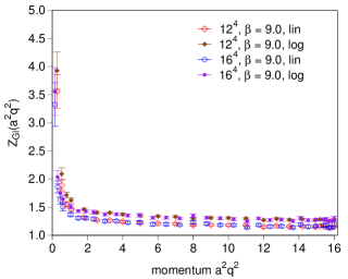
Figure 7: The bare gluon dressing function for $\beta=6.0$ (left) and $\beta=9.0$ (right) versus the lattice momentum squared. The data is for two lattice sizes. Filled symbols are for the logarithmic definition and open symbols for the linear.

This is even better seen in Fig. 8 where the ratio

$$C_{\rm gluon}(q^{2})=\frac{D^{\rm(lin)}(q^{2})}{D^{\rm(log)}(q^{2})}$$ (41)

is shown versus momentum. For both $\beta$-values, we observe the ratio to be constant within statistical errors over the whole momentum region, and to depend on $\beta$. Thus the bare gluon propagators differ for the two definitions but are related to each other by a finite $\beta$-dependent multiplicative renormalization constant. As a consequence both definitions will lead to the same propagator when renormalized in a MOM scheme, the latter being defined by the condition that the propagator equals its tree-level expression at some subtraction momentum $q^{2}=\mu^{2}$. Of course, this multiplicative renormalizability has been numerically demonstrated here only for finite volume and corresponding restricted momentum range under consideration.

  

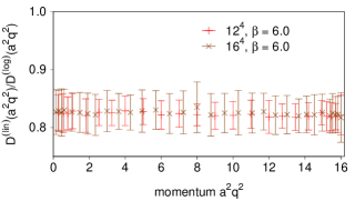
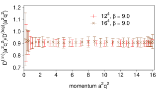
Figure 8: The ratio $C_{\rm gluon}$ acc. to (41) relating the gluon propagator for the two definitions of the gluon field. Data is for $\beta=6.0$ (left) and $\beta=9.0$ (right) on a $12^{4}$ and $16^{4}$ lattice.

Also for ghost propagator we clearly see the offset between the dressing functions for the logarithmic and linear definitions (see Fig. 9 for the data at $\beta=6.0$ and $9.0$).

  

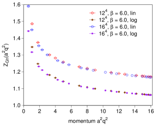
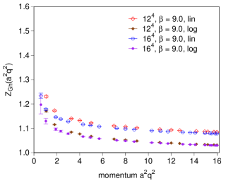
Figure 9: The bare ghost dressing functions versus the lattice momentum squared. Data is for $\beta=6.0$ (left) and $\beta=9.0$ (right) and two lattice sizes. Filled (open) symbols are for the logarithmic (linear) definition.

Similar to Fig. 8, in Fig. 10 we show the ratio

$$C_{\rm ghost}(q^{2})=\frac{G^{\rm(lin)}(q^{2})}{G^{\rm(log)}(q^{2}}$$ (42)

as a function of the momentum squared $q^{2}$. For both values of $\beta$, we see an approximately constant ratio over a wide momentum range. The deviation seen at the smallest momenta for $\beta=9.0$ remains within statistical errors. In Table 5 we list the values for $C_{\rm gluon}$ and $C_{\rm ghost}$. As expected, their ratios happen to be related as

$$C_{\rm gluon}\cdot C_{\rm ghost}^{2}\approx 1\,.$$ (43)

This implies that the ghost-gluon coupling $\alpha^{\mathsf{MM}}_{s}(q^{2})$ (see Section V.3) determined directly from the gluon and ghost dressing functions is the same for the logarithmic or linear definition.

  

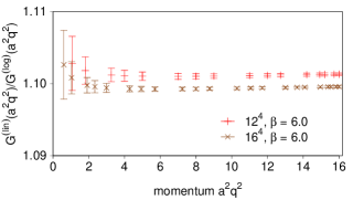
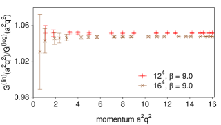
Figure 10: The ratio $C_{\rm ghost}$ acc. to (42) relating the ghost propagator for the two definitions of the gluon field and the Faddeev-Popov operator, respectively, for $12^{4}$ and $16^{4}$ lattices generated at $\beta=6.0$ (left) and $\beta=9.0$ (right).

Table 5: The ratios $C_{\rm gluon}$ and $C_{\rm ghost}$ [Eqs. (41) and (42)] for the linear and logarithmic definition.

lattice	$\beta$	$C_{\rm gluon}$	$C_{\rm ghost}$
$12^{4}$	$6.0$	$0.82\pm 0.02$	$1.1013\pm 0.0007$
$12^{4}$	$9.0$	$0.91\pm 0.03$	$1.0510\pm 0.0010$
$16^{4}$	$6.0$	$0.82\pm 0.03$	$1.0996\pm 0.0006$
$16^{4}$	$9.0$	$0.91\pm 0.04$	$1.0460\pm 0.0040$

V.2 Finite-volume and lattice discretization effects

Next we analyze discretization and finite-volume effects. In this section the discussion will be restricted to the propagators for the logarithmic definition. Corresponding data for ghost-gluon coupling, $\alpha^{\mathsf{MM}}_{s}(q^{2})$, is then discussed in the next section.

When checking lattice discretization artifacts, we fix the physical volume such that it approximately equals that of all data for different $a(\beta)$. In contrast, finite-volume effects will be analyzed for a fixed $\beta$ varying the lattice size.

To analyze lattice discretization artifacts for the gluon and ghost propagators we compare their renormalized dressing functions at $\beta=5.8$, 6.0 and 6.2. Using the respective lattice sizes $16^{4}$, $24^{4}$ and $32^{4}$, the physical volume is then roughly $V\simeq(2.2\mathrm{~{}fm})^{4}$. For the renormalization we chose $\mu\approx 3.2\mathrm{~{}GeV}$, which we find lies well below the momenta where discretization artifacts could affect the renormalization. The corresponding data is shown in Fig. 11 suggesting that, with respect to precision of the data, lattice discretization artifacts are reasonably small.

  

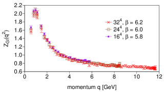
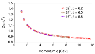
Figure 11: Renormalized gluon (left) and ghost dressing function (right) for the logarithmic definition and various lattice spacings $a=a(\beta)$. The physical volume is fixed to $V=(2.2\mathrm{~{}fm})^{4}$. Data has been renormalized at $q=\mu\approx 3.2\mathrm{~{}GeV}$.

To check finite-volume effects we choose $\beta=6.0$ and vary the lattice size from $16^{4}$, $24^{4}$ and $32^{4}$. This has been arranged for the data in Fig. 12 where we compare the renormalized gluon and ghost dressing functions. One clearly sees that finite-volume effects are negligible above $1\mathrm{~{}GeV}$, the momentum where the gluon dressing function has its maximum. At ${\cal O}(1)\mathrm{~{}GeV}$ and below a slight volume dependence becomes visible. The overall behavior resembles that what has been observed for $A^{\rm(lin)}$ in other studies. In order to see these effects well below $1\mathrm{~{}GeV}$, much larger lattices are needed, for example, as those studied for the linear definition in Bogolubsky et al. (2009a).

  

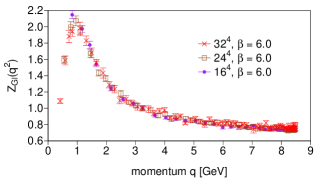
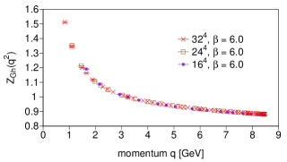
Figure 12: The renormalized gluon (left) and ghost dressing function (right) for the logarithmic definition. The data is for a fixed lattice spacing ($\beta=6.0$) but three different volumes $V$. The renormalization point is at $\mu\approx 3.2\mathrm{~{}GeV}$.

V.3 The running coupling

The running coupling $\alpha_{s}(q^{2})$ for Yang-Mills theories can be defined in various ways. Here we use the coupling of ghost-gluon vertex in a particular (minimal) MOM scheme (see von Smekal et al. (1997); Alkofer and von Smekal (2001) as well as the more recent papers von Smekal et al. (2009); Sternbeck et al. (2009)). It can be defined in terms of the bare, i.e., unrenormalized gluon and ghost dressing functions $Z_{\rm Gl}$ and $Z_{\rm Gh}$ as follows:

$$\alpha^{\mathsf{MM}}_{s}(q^{2})=\frac{g_{0}^{2}}{4\pi}Z_{\rm Gl}(a^{2},q^{2})Z_{\rm Gh}^{2}(a^{2},q^{2})\,.$$ (44)

It is a renormalization-group invariant quantity, i.e., shifting the cutoff $a^{-1}$ or transforming the right hand side into renormalized quantities and changing their subtraction momentum $\mu$ within the given MOM scheme should not alter $\alpha^{\mathsf{MM}}_{s}(q^{2})$. Therefore, we can compute it directly from the bare lattice dressing functions at an arbitrary large enough cutoff-value $a^{-1}(\beta)$, as long as multiplicative renormalization is ensured and additive lattice artifacts are suppressed. In what follows we shall omit the superscript $\mathsf{MM}$ for simplicity.

First, we check effects due to the lattice discretization and the finite volume. In order to investigate lattice discretization effects we present on the left hand side of Fig. 13 the running coupling $\alpha_{s}(q^{2})$ for different lattice spacings but fixed physical volume [as above we choose again $V=(2.2\mathrm{~{}fm})^{4}$]. Apparently, there are some systematic lattice discretization effects, suggesting that for the given (rather small) $\beta$ additive lattice artifacts are small but not negligible. This is in agreement with the findings in Sternbeck et al. (2009). These artifacts should disappear for large $\beta$. On the right hand side of Fig. 13, we show data for different physical lattices sizes but fixed lattice spacing [again we choose $\beta=6.0$]. Based on that figure we have to conclude that finite-volume effects seem to be negligible for the considered momentum range.

  

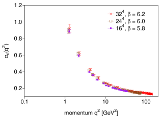
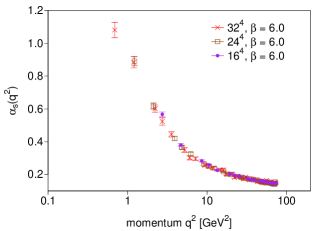
Figure 13: $\alpha_{s}(q^{2})$ for the logarithmic definition as a function of physical momentum squared. Left: for three lattice spacings $a=a(\beta)$ but fixed physical volume $V=(2.2\mathrm{~{}fm})^{4}$. Right: for different volumes $V$ but fixed lattice spacing $a=a(\beta=6.0)$.

In Fig. 14 we finally compare the coupling for the logarithmic and the linear definition. We decided to show data for various lattice sizes and $\beta$ values in a single plot to demonstrate that altogether the data for the two definitions matches up almost completely. Regrettably, there are some small deviations due to the different lattice spacings and volumes, but this should be expected. The almost perfect overlap of the two curves agrees, of course, well with what we saw above for the ratios of the propagators (see Eq. (43)). That is, $\alpha_{s}(q^{2})$ will not differ calculated either for the standard (linear) approach (as in Sternbeck et al. (2009)) or for the logarithmic approach as done here. Unfortunately, we cannot say which approach comes with the smaller lattice discretization artifacts. This is left for a future study.

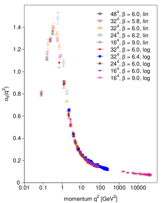
Figure 14: Running coupling for various lattice sizes and $\beta$-values. Filled symbols are for the logarithmic definition, while open symbols are for the linear one.

VI Comparison with NSPT

We now turn to the NSPT results of Di Renzo et al. (2010a); Di Renzo et al. (2011); Di Renzo et al. (2010b) which below we will compare to our data. Let us start first with some facts on NSPT.

NSPT is a numerical approach to lattice perturbation theory that allows to circumvent the difficulties of the standard diagrammatic approach and facilitates automatized perturbative calculations. It has its roots in stochastic quantization and is based on a modified Langevin equation equipped with stochastic gauge fixing corresponding to a gauge fixing term $(\partial_{\mu}A_{\mu})^{2}/(2\xi)$ at finite $\xi$ . For our purposes it is actually a hierarchy of first-order evolution equations associated with the various parts of the gauge field when expanded in terms of the lattice coupling $g_{0}\propto 1/\sqrt{\beta}$:

$$U_{x,\mu} =1+\sum_{l\geq 1}\beta^{-l/2}U^{(l)}_{x,\mu}\,,$$ (45)

$$A^{\rm(log)}_{x+\frac{\hat{\mu}}{2},\mu} =\sum_{l\geq 1}\beta^{-l/2}A^{(l)}_{x+\frac{\hat{\mu}}{2},\mu}\,,$$

From a numerical point of view, these different parts, representing first, second, third etc. orders, are separately dealt within the code. The maximal addressable order of perturbation theory is thus limited by the available computing resources (cpu time and memory).

The Langevin simulation is implemented in an Euler scheme with a finite evolution time step. Lattice observables, in our case the ghost Di Renzo et al. (2010a) and gluon Di Renzo et al. (2011) propagators, are evaluated taking the long-time average, order by order in a loop expansion in even powers of $g_{0}$. Contributions from odd powers vanish within the statistical errors. As for any Langevin simulation, one then has to take the limit to vanishing time step. This is in addition to the continuum limit and the limit of infinite volume.

Regardless of this, NSPT results for a finite lattice volume can be confronted directly with standard MC results for a given $\beta$, supposed the lattice size and definition of the studied observable is the same in both approaches.

But before such a comparison is possible, the limit $\xi\to 0$ (minimal Landau gauge) has to be taken. This is arranged such that a sequence of configurations (separated by ${\cal O}(50)$ Langevin time steps) undergoes a Fourier-accelerated gauge-fixing procedure, after which the individual gluon fields, $A^{(l)}_{\mu}$, each associated with particular perturbative order ($g_{0}^{l}$), are transversal within machine precision.

As in standard lattice perturbation theory, an expanded version of the logarithmic relation between the gluon fields and the transporters (compare (3)) is taken into account up to the maximal order of perturbation theory addressed in the given case. Correspondingly, the gauge functional and the structure of the Faddeev-Popov operator are the same as in Eqs. (IV.2) and (IV.2).

The gluon two-point function in $n$-loop order is then defined as a convolution of the bilinears of gluon fields (in momentum space) in complementary orders:

$$\delta^{ab}D_{\mu\nu}^{(n)}(p(k))=\left\langle\,\sum_{l=1}^{2n+1}\left[\widetilde{A}^{a,(l)}_{\mu}(k)\,\widetilde{A}^{b,(2n+2-l)}_{\nu}(-k)\right]\,\right\rangle_{U}\,.$$ (46)

The Faddeev-Popov operator (explicitly written in Eq. (IV.2) up to fourth order) can be expanded in terms of products of various $A^{(l)}$, with the term $M^{(n)}$ collecting all terms of order $g_{0}^{n}$. This structure allows to express the inverse of the Faddeev-Popov operator also as an expansion in orders of $g_{0}$ in a recursive way, without the need of explicitly inverting any other than the zeroth order term, $M^{(0)}=\Delta$ (the Laplacian).

A reasonable “convergence” of the NSPT results up to few loops (three or four are available now) requires a small bare coupling $g_{0}$, i.e., a large $\beta$. However, the bare coupling $g_{0}$ is known to be a poor expansion parameter Lepage and Mackenzie (1993). One can speed up convergence by “boosting”, i.e., trading the bare coupling constant by an effective “boosted” coupling $g_{b}^{2}=g_{0}^{2}/P_{\mathrm{pert}}(g_{0}^{2})>g_{0}^{2}$, where $P_{\mathrm{pert}}$ is defined by the average perturbative plaquette. Its expansion is determined within the Langevin simulations, along with the propagators. The effect of the larger boosted coupling is overcompensated by the rapid decay of the expansion coefficients with respect to $g_{b}^{2}$.

  

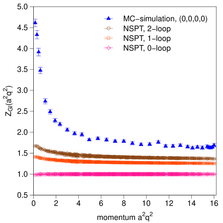
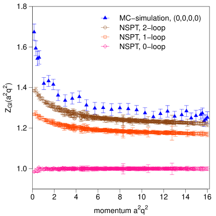
Figure 15: Comparison of MC with NSPT results for the bare gluon dressing function at (cumulative) tree, 1-loop and 2-loop level at $\beta=6.0$ (left) and $\beta=9.0$ (right). The lattice size is $16^{4}$.

  

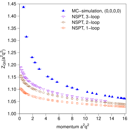
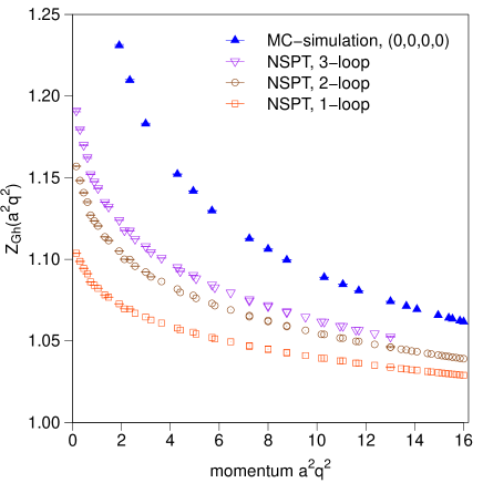
Figure 16: Comparison of MC with NSPT results for the bare ghost dressing function at (cumulative) 1-loop, 2-loop and 3-loop level at $\beta=6.0$ (left) and $\beta=9.0$ (right). The lattice size is $16^{4}$.

  

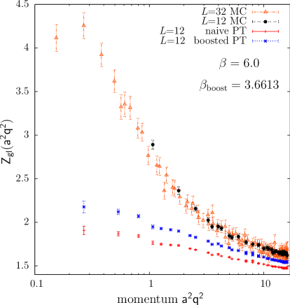
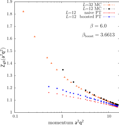
Figure 17: Comparison of naive and boosted LPT (based on NSPT) with MC data for a $12^{4}$ lattice at $\beta=6.0$. Left: the bare gluon dressing function up to 4-loop. Right: the bare ghost dressing function up to 3-loop. We also include MC data for a $32^{4}$ lattice.

  

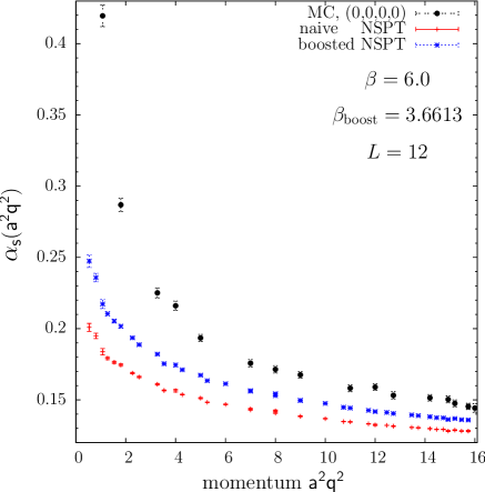
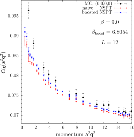
Figure 18: Comparing naive and boosted LPT (based on NSPT) data for the running coupling constant $\alpha_{s}(q^{2})$ to corresponding MC data for a $12^{4}$ lattice. Left: $\beta=6.0$. Right: $\beta=9.0$. For the LPT data, the gluon (ghost) dressing function up to 4-loop (3-loop) accuracy has been included.

We now compare our data for the logarithmic definition to the NSPT results of Di Renzo et al. (2010a); Di Renzo et al. (2011); Di Renzo et al. (2010b).

One should be aware that on small lattices, with sizes like $12^{4}$ or $16^{4}$, and for the larger $\beta$ values, the Monte Carlo lattice gauge fields will be in a pseudo-deconfinement phase. This can be monitored by the “spatially” averaged Polyakov loops, actually in all four directions. It is well-known that the agreement of Monte Carlo results with standard LPT requires that the Monte Carlo simulation is guaranteed to stay in the trivial Polyakov sector Damm et al. (1998). For $SU(3)$ this means, that the average Polyakov loops in all four directions have to be located in the sector of predominantly real values. Let us denote averages in this sector by the corresponding phases $(0,0,0,0)$, in distinction to results obtained from Monte Carlo configurations without taking notice of the Polyakov sector. Note that one can easily switch between the Polyakov loop sectors by applying global $Z(3)$ transformations on all link variables attached to and pointing forward, orthogonal to an arbitrary 3D plane. While at $\beta=9.0$ the MC results for the gluon and ghost dressing functions clearly depend on the Polyakov loop sector, for $\beta=6.0$ the Polyakov loop values fluctuate closely around the origin of the complex plane, i.e., in the confined phase. In this case the choice of a sector should not influence the behavior of the propagators or dressing functions. In what follows, for the detailed comparison all Monte Carlo configurations at $\beta=9.0$ have been flipped to the real sector $(0,0,0,0)$ if necessary, before the gauge fixing has been performed.

Let us first confront the tree level and the cumulative one-loop and two-loop contributions to the gluon dressing function with the results from Monte Carlo simulations (see Fig. 15). The simulations have been performed for a $16^{4}$ lattice at $\beta=6.0$ and $\beta=9.0$, the same values as for the NSPT results. For the reader’s convenience, we present the NSPT data the same way the Monte Carlo data has been present above. When looking at the data in Fig. 15 we see the NSPT results approaches the MC data with increasing loop order. As expected though, this is less the case for $\beta=6.0$, but for $\beta=9.0$ the NSPT data almost approaches the MC data.

Similar we see for the bare ghost dressing function in Fig. 16. For this the speed of convergence of the NSPT results can be assessed from the difference between two-loop and three-loop Di Renzo et al. (2010a). The three-loop result is already very close to the MC result for $\beta=9.0$ and at the largest available momenta.

Next we illustrate the effect of “boosting” the perturbative expansion. For this we use the currently available NSPT results (up to four/two loops ($L\leq 12$/$L=16,20,32$) for the gluon propagator and up three loops ($L\leq 20$) for the ghost propagator) and confront them with corresponding MC data. This is shown in Fig. 17 where also the bare inverse coupling $\beta$ and its boosted value $\beta_{\mathrm{boost}}$ are given. As expected, boosting moves the NSPT data closer to the MC results, but they cannot be reached, certainly not at $\beta=6.0$.

Last but not least, the running coupling, $\alpha_{s}(q^{2})$, as calculated from the NSPT dressing functions, both summed up to the available orders, is compared to the Monte Carlo results at $\beta=6.0$ and $9.0$. The corresponding data is shown in Fig. 18, again for naive and boosted perturbation theory. We see that the running coupling from Monte Carlo simulations is approached from below up to 7% for $\beta=6.0$ and practically approached within the present errors for $\beta=9.0$.

Concluding this section, one can say that our MC results for the logarithmic approach to Landau gauge propagators support the validity of the NSPT calculation for the gluon as well as for the ghost propagator. In fact, the NSPT results do not coincide with the MC data but they become closer with increasing order of the perturbative expansion. Also, the difference between the NSPT and MC data becomes smaller for larger $\beta$, suggesting the difference to be related to nonperturbative effects NSPT results cannot provide.

VII Conclusions

In this paper we have studied an alternative approach to compute the $SU(3)$ Landau gauge gluon and ghost propagators on the lattice. This approach uses a logarithmic ansatz [Eq. (3)] for the definition of the lattice gluon fields from a given gauge field configuration. It is thus best suited to compare lattice MC data for these propagators with results from NSPT. We have started the task by first exploring some options for an efficient algorithm that fixes gauge field configurations to Landau gauge for the logarithmic case. We find a multigrid-accelerated gradient method with a preconditioning step of simulated annealing and subsequent overrelaxation, applied to the linearly defined gluon field, to be a good choice. The method is also easy parallelizable.

With this algorithm at our disposal we have compared the bare lattice propagators for the logarithmic and the linear definition of gluon fields. As expected, we see them to differ by multiplicative factors that depend on $\beta$. Those factors are such that they perfectly cancel when one considers $\alpha_{s}(q^{2})$. Apart from some small lattice discretization artifacts, data for the running coupling matches up almost completely, as it should for a renormalization-group invariant object. It is thus also an ideal quantity to assess discretization artifacts.

For the logarithmic definition we have checked Gribov copy, finite-size and lattice discretization effects, and find them to be small for momenta $q>1\mathrm{~{}GeV}$.

Finally we have compared our MC data for the logarithmic definition with results from NSPT. These are available up to four loops for the gluon propagator, and up to three loops for the ghost propagator. We find a reasonable convergence at large momentum. Note that for this it is important that during the MC process the gauge field configurations are kept in the correct (real-valued) Polyakov loop sector. For large $\beta$, these may easily pass a pseudo-deconfinement phase transition.

Our results altogether support universality with respect to the two lattice realizations of $SU(3)$ Landau gauge theory studied herein. In as far this universality persist in the low-momentum region remains to be seen.

We emphasize that the universality of different lattice definitions we have observed in this paper assumes a unique Landau gauge fixing based on the (global) minimization of a corresponding gauge functional. For an alternative view of dealing with the Gribov copy problem see Refs. Maas (2010); Maas et al. (2010).

Appendix A Multigrid Fourier-accelerated gauge-fixing

For our implementation of a parallel version of the Fourier-accelerated gauge fixing we follow Goodman and Sokal Goodman and Sokal (1986, 1989) using the representation of the Fourier transformation of $1/q^{2}$ in position space:

$$\hat{F}^{-1}\left[\frac{q_{\rm max}^{2}}{q^{2}}\hat{F}\left[(\sum_{\mu}\partial_{\mu}{}^{g}\!A^{\rm(log)}_{\mu})(x)\right]\right]$$ (47)

$$= q_{\rm max}^{2}~{}\Delta^{-1}(\sum_{\mu}\partial_{\mu}{}^{g}\!A^{\rm(log)}_{\mu})(x)\,.$$

This leads us to a simple inversion of the Laplacian, i.e., to solving the 4D Poisson equation

$$-\left(\Delta v\right)(x)=\left(\sum_{\mu}\partial_{\mu}A^{\rm(log)}_{\mu}\right)(x)$$ (48)

using for example the local Jacobi method. To avoid critical slowing down inherent to this method we use the multigrid algorithm by solving (48) successively on the original (fine) lattice and on several coarser lattices. In order to use our multigrid algorithm for various lattice sizes we implement the multigrid with a symmetric lattice decomposition.

On each sublattice one has to solve a system of linear equations

$$A^{h}v^{h}=f^{h}\,,$$ (49)

where the superscript $h$ describes the respective lattice spacing $h=a,2a,4a,8a,..$. Comparing with (48) we can see that $A^{a}=\Delta$. For switching between the lattices one defines interpolation matrices $I$ as

$$\begin{split}&\hskip 17.07182ptA^{h^{\prime}}=I_{h^{\prime},h}A^{h}\left[I_{h^{\prime},h}\right]^{T}\\ &v^{h^{\prime}}=I_{h^{\prime},h}v^{h}\hskip 5.69046pt,\hskip 5.69046ptf^{h^{\prime}}=I_{h^{\prime},h}f^{h}\end{split}$$ (50)

and projection matrices $P$

$$\begin{split}&\hskip 17.07182ptA^{h}=P_{h,h^{\prime}}A^{h^{\prime}}\left[P_{h,h^{\prime}}\right]^{T}\\ &v^{h}=P_{h,h^{\prime}}v^{h^{\prime}}\hskip 5.69046pt,\hskip 5.69046ptf^{h}=P_{h,h^{\prime}}f^{h^{\prime}}\,.\end{split}$$ (51)

$h^{\prime}$ always denotes the lattice with the finer spacing while $h$ denotes the coarser lattice. The matrix structure (in terms of the lattice sites) of these equations is left implicit. The projection matrices are the transposed interpolation matrices (with respect to the indices pointing to lattice sites)

$$P_{h,h^{\prime}}=\left[I_{h^{\prime},h}\right]^{T}\,.$$ (52)

The matrices were chosen in the way that the operator $A^{h^{\prime}}$ got the same structure on all sublattices (i.e. $A^{h^{\prime}}=\Delta^{h^{\prime}}$). In practice, the multigrid algorithm is realized by jumping between the finest and various coarser lattices. This is summarized in the flow chart in Fig. 19.

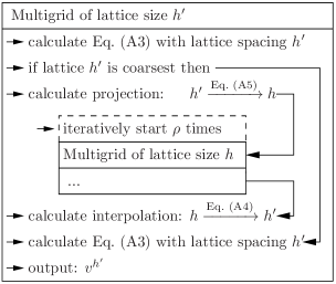
Figure 19: Flow chart illustrating our multigrid algorithm.

Solving Eq. (49) before the projection is called pre-smoothing, post-smoothing after the interpolation, respectively Briggs et al. (2000). To solve Eq. (49) we use the Jacobi method with a fixed number of $20$ iterations. Hence we did not solve equation Eq. (49) at high numerical accuracy on the sublattices. Nevertheless, the accuracy of this calculation seems to have only a minor influence on the total number of iterations needed to fix the Landau gauge. For the parameter $\rho$ we chose the value $\rho=2$, i.e., the so called $W$-cycle.

References

- Cucchieri and Mendes (2008a) A. Cucchieri and T. Mendes, Phys. Rev. Lett. 100, 241601 (2008a), eprint 0712.3517.
- Cucchieri and Mendes (2008b) A. Cucchieri and T. Mendes, Phys. Rev. D78, 094503 (2008b), eprint 0804.2371.
- Bogolubsky et al. (2009a) I. L. Bogolubsky, E.-M. Ilgenfritz, M. Müller-Preussker, and A. Sternbeck, Phys. Lett. B676, 69 (2009a), eprint 0901.0736.
- Bornyakov et al. (2010) V. G. Bornyakov, V. K. Mitrjushkin, and M. Müller-Preussker, Phys. Rev. D81, 054503 (2010), eprint 0912.4475.
- Gribov (1978) V. N. Gribov, Nucl. Phys. B139, 1 (1978).
- Zwanziger (1994) D. Zwanziger, Nucl. Phys. B412, 657 (1994).
- Kugo and Ojima (1979) T. Kugo and I. Ojima, Prog. Theor. Phys. Suppl. 66, 1 (1979).
- Fischer et al. (2007) C. S. Fischer, A. Maas, J. M. Pawlowski, and L. von Smekal, Annals Phys. 322, 2916 (2007), eprint hep-ph/0701050.
- von Smekal (2008) L. von Smekal (2008), eprint 0812.0654.
- Maas (2010) A. Maas, Phys. Lett. B689, 107 (2010), eprint 0907.5185.
- Maas et al. (2010) A. Maas, J. M. Pawlowski, D. Spielmann, A. Sternbeck, and L. von Smekal, Eur. Phys. J. C68, 183 (2010), eprint 0912.4203.
- Cucchieri et al. (2005) A. Cucchieri, T. Mendes, and A. R. Taurines, Phys. Rev. D71, 051902 (2005), eprint hep-lat/0406020.
- Sternbeck et al. (2006) A. Sternbeck, E.-M. Ilgenfritz, M. Müller-Preussker, A. Schiller, and I. L. Bogolubsky, PoS LAT2006, 076 (2006), eprint hep-lat/0610053.
- Bowman et al. (2007) P. O. Bowman et al., Phys. Rev. D76, 094505 (2007), eprint hep-lat/0703022.
- Braun et al. (2010) J. Braun, H. Gies, and J. M. Pawlowski, Phys. Lett. B684, 262 (2010), eprint 0708.2413.
- Becirevic et al. (2000) D. Becirevic et al., Phys. Rev. D61, 114508 (2000), eprint hep-ph/9910204.
- Boucaud et al. (2006) P. Boucaud et al., Phys. Rev. D74, 034505 (2006), eprint hep-lat/0504017.
- Boucaud et al. (2005) P. Boucaud et al., Phys. Rev. D72, 114503 (2005), eprint hep-lat/0506031.
- Sternbeck et al. (2009) A. Sternbeck et al., PoS LAT2009, 210 (2009), eprint 1003.1585.
- Blossier et al. (2010) B. Blossier et al. (ETM), Phys. Rev. D82, 034510 (2010), eprint 1005.5290.
- Boucaud et al. (2009) P. Boucaud et al., Phys. Rev. D79, 014508 (2009), eprint 0811.2059.
- Alkofer et al. (2010) R. Alkofer, G. Eichmann, A. Krassnigg, and D. Nicmorus, Chin. Phys. C34, 1175 (2010), eprint 0912.3105.
- Giusti et al. (1998) L. Giusti, M. L. Paciello, S. Petrarca, B. Taglienti, and M. Testa, Phys. Lett. B432, 196 (1998), eprint hep-lat/9803021.
- Petrarca et al. (1999) S. Petrarca, L. Giusti, M. L. Paciello, B. Taglienti, and M. Testa, Nucl. Phys. Proc. Suppl. 73, 862 (1999), eprint hep-lat/9809048.
- Furui and Nakajima (1999) S. Furui and H. Nakajima, Nucl. Phys. Proc. Suppl. 73, 865 (1999), eprint hep-lat/9809080.
- Cucchieri and Karsch (2000) A. Cucchieri and F. Karsch, Nucl. Phys. Proc. Suppl. 83, 357 (2000), eprint hep-lat/9909011.
- Bogolubsky and Mitrjushkin (2002) I. L. Bogolubsky and V. K. Mitrjushkin (2002), eprint hep-lat/0204006.
- Bogolubsky et al. (2009b) I. L. Bogolubsky, E.-M. Ilgenfritz, M. Müller-Preussker, and A. Sternbeck, PoS (LAT2009) 237 (2009b), eprint 0912.2249.
- Di Renzo et al. (2010a) F. Di Renzo, E.-M. Ilgenfritz, H. Perlt, A. Schiller, and C. Torrero, Nucl. Phys. B831, 262 (2010a), eprint 0912.4152.
- Di Renzo et al. (2011) F. Di Renzo, E.-M. Ilgenfritz, H. Perlt, A. Schiller, and C. Torrero, Nucl. Phys. B842, 122 (2011), eprint 1008.2617.
- von Smekal et al. (1997) L. von Smekal, A. Hauck, and R. Alkofer, Phys. Rev. Lett. 79, 3591 (1997), eprint hep-ph/9705242.
- von Smekal et al. (2007) L. von Smekal, D. Mehta, A. Sternbeck, and A. G. Williams, PoS LAT2007, 382 (2007), eprint 0710.2410.
- Neuberger (1986) H. Neuberger, Phys. Lett. B175, 69 (1986).
- Neuberger (1987) H. Neuberger, Phys. Lett. B183, 337 (1987).
- Sternbeck and von Smekal (2010) A. Sternbeck and L. von Smekal, Eur. Phys. J. C68, 487 (2010), eprint 0811.4300.
- Nakajima and Furui (2000) H. Nakajima and S. Furui, Nucl. Phys. A680, 151 (2000), eprint hep-lat/0004023.
- Furui and Nakajima (2004a) S. Furui and H. Nakajima, Phys. Rev. D69, 074505 (2004a), eprint hep-lat/0305010.
- Furui and Nakajima (2004b) S. Furui and H. Nakajima, Phys. Rev. D70, 094504 (2004b).
- Furui and Nakajima (2006) S. Furui and H. Nakajima, Few Body Syst. 40, 101 (2006), eprint hep-lat/0503029.
- Rothe (1997) H. J. Rothe, World Sci. Lect. Notes Phys. 59, 1 (1997).
- von Smekal et al. (2009) L. von Smekal, K. Maltman, and A. Sternbeck, Phys. Lett. B681, 336 (2009), eprint 0903.1696.
- Chetyrkin and Retey (2000) K. G. Chetyrkin and A. Retey (2000), eprint hep-ph/0007088.
- Chetyrkin (2005) K. G. Chetyrkin, Nucl. Phys. B710, 499 (2005), eprint hep-ph/0405193.
- Damm et al. (1998) G. Damm, W. Kerler, and V. K. Mitrjushkin, Phys. Lett. B433, 88 (1998), eprint hep-lat/9802028.
- Cabibbo and Marinari (1982) N. Cabibbo and E. Marinari, Phys. Lett. B119, 387 (1982).
- Bali et al. (1996) G. S. Bali, V. Bornyakov, M. Müller-Preussker, and K. Schilling, Phys. Rev. D54, 2863 (1996), eprint hep-lat/9603012.
- Schemel (2006) P. Schemel, Diploma thesis, Humboldt University Berlin, Germany, see http://pha.physik.hu-berlin.de - Theses (2006).
- Bogolubsky et al. (2007) I. L. Bogolubsky, V. G. Bornyakov, G. Burgio, E.-M. Ilgenfritz, V. K. Mitrjushkin, M. Müller-Preussker, and P. Schemel, PoS LAT2007, 318 (2007), eprint 0710.3234.
- Davies et al. (1988) C. T. H. Davies et al., Phys. Rev. D37, 1581 (1988).
- Nakajima et al. (2001) H. Nakajima, S. Furui, and A. Yamaguchi, Nucl. Phys. Proc. Suppl. 94, 558 (2001), eprint hep-lat/0010083.
- Goodman and Sokal (1986) J. Goodman and A. D. Sokal, Phys. Rev. Lett. 56, 1015 (1986).
- Cucchieri and Mendes (1998) A. Cucchieri and T. Mendes, Phys. Rev. D57, 3822 (1998), eprint hep-lat/9711047.
- Necco and Sommer (2002) S. Necco and R. Sommer, Nucl. Phys. B622, 328 (2002), eprint hep-lat/0108008.
- Sternbeck et al. (2005) A. Sternbeck, E.-M. Ilgenfritz, M. Müller-Preussker, and A. Schiller, Phys. Rev. D72, 014507 (2005), eprint hep-lat/0506007.
- Leinweber et al. (1999) D. B. Leinweber, J. I. Skullerud, A. G. Williams, and C. Parrinello, Phys. Rev. D60, 094507 (1999), eprint hep-lat/9811027.
- de Soto and Roiesnel (2007) F. de Soto and C. Roiesnel, JHEP 09, 007 (2007), eprint 0705.3523.
- Bakeev et al. (2004) T. Bakeev, E.-M. Ilgenfritz, M. Müller-Preussker, and V. K. Mitrjushkin, Phys. Rev. D69, 074507 (2004), eprint hep-lat/0311041.
- Bogolubsky et al. (2008) I. L. Bogolubsky, V. G. Bornyakov, G. Burgio, E.-M. Ilgenfritz, M. Müller-Preussker, and V. K. Mitrjushkin, Phys. Rev. D77, 014504 (2008), eprint 0707.3611.
- Bornyakov et al. (2009) V. G. Bornyakov, V. K. Mitrjushkin, and M. Müller-Preussker, Phys. Rev. D79, 074504 (2009), eprint 0812.2761.
- Alkofer and von Smekal (2001) R. Alkofer and L. von Smekal, Phys. Rept. 353, 281 (2001), eprint hep-ph/0007355.
- Di Renzo et al. (2010b) F. Di Renzo, E.-M. Ilgenfritz, H. Perlt, A. Schiller, and C. Torrero (2010b), eprint 1012.1764.
- Pawlowski et al. (2010) J. M. Pawlowski, D. Spielmann, and I.-O. Stamatescu, Nucl. Phys. B830, 291 (2010), eprint 0911.4921.
- Lepage and Mackenzie (1993) G. P. Lepage and P. B. Mackenzie, Phys. Rev. D48, 2250 (1993), eprint hep-lat/9209022.
- Goodman and Sokal (1989) J. Goodman and A. D. Sokal, Phys. Rev. D40, 2035 (1989).
- Briggs et al. (2000) W. L. Briggs, V. E. Henson, and S. F. McCormick, A Multigrid Tutorial, 2nd edition, SIAM (2000).