Spin entanglement of two spin-$\frac{1}{2}$ particles in a classical gravitational field

Abstract

The effect of a classical gravitational field on the spin entanglement of a system of two spin-$\frac{1}{2}$ particles moving in the curved spacetime is discussed. The system is described by a two-particle Gaussian wave packet represented in the momentum space and both the acceleration of the system and the curvature of the spacetime cause to produce a Wigner rotation acting on the wave packet as it moves along a path in the curved spacetime. By calculating the reduced density operator at a final point, we focus on the spin entanglement of the system. In a spherically symmetric and static gravitational field, for example a charged black hole, there can be particular paths on which the Wigner rotation is trivial and so the initial reduced density matrix remains intact. This causes the spin entanglement to be invariant during the motion. The spin entanglement descends to zero by increasing the angular velocity of the mean centroid of the system as well increasing the proper time during which the centroid moves on its circular path around the center.

I Introduction

The field of quantum information has made rapid progress in recent years. It is important to study all those processes that might have an effect on quantum entanglement. Special relativistic effects on quantum entanglement and quantum information is investigated by many authors peres ; trashima ; alsing ; ahn ; lee ; kim ; ging ; li . It is shown that though Lorentz transformations can change the entanglement of the spins of massive particles, the total entanglement is invariant for inertial observers. Some authors studied the entanglement between two modes of a free Dirac field as seen by two relatively accelerated observers mann ; pan . This entanglement is degraded by the Unruh effect and asymptotically reaches a non-vanishing minimum value in the infinite acceleration limit. Furthermore, using the formalism of quantum fields in curved spacetimes, extension of the quantum entanglement and teleportation to the gravitational field in four-dimensional spacetimes, as well in higher dimensional black hole spacetimes is discussed shen ; ge . There exists another approach for discussing the effect of gravitational field on quantum information in which, using the concept of local inertial frames, the special relativistic considerations is extended to general relativity. Using this approach and considering a wave packet for the system, Terashima and Ueda discussed a mechanism of spin rotation caused by spacetime curvature for spin-$\frac{1}{2}$ particles moving in a gravitational field terashima3 . It is shown that this effect gives rise to a spin entropy production that is unique to general relativity. This means that even if the spin state of the particle is pure at one spacetime point, it becomes mixed at another spacetime point. In the same manner, the gravitational spin entropy production for particles with arbitrary spin moving in a curved spacetime is discussed nasr1 .

In the present article, regarding the latter approach, we discuss the effect of a gravitational field on the spin entanglement of a system consisting of two spin-$\frac{1}{2}$ particles moving in the gravitational field. For theoretical reasons, it may be interesting to quantify the entanglement for such a system. We describe the system by a two-particle wave packet represented in the momentum space with a definite width around the momentum of a mean centroid. We consider the mean centroid for describing the motion of the system in the gravitational field which is a classic field in our approach. Thus we require to assume that the curvature of the gravitational field does not change drastically within the spacetime scale of the wave packet. Using the concept of local inertial frames it turns out that both the acceleration of the centroid and the curvature of the gravitational field cause to produce a Wigner rotation that affects the wave packet. We confine the argument to a static spherically symmetric gravitational field such as a charged black hole which because of the mathematical form of its metric, allows us to present a detailed argument. At a given initial point in the curved spacetime, the momenta of the particles are taken to be separable, while the spin part is chosen to be entangled as the Bell states. By calculating the reduced density operator, we focus on the spin entanglement of the system as moves on a circular path around the center. In the present problem, one can more closely investigate how a central massive charged body affects a quantum communication that takes place around it.

II Wigner rotation for two-particle states moving in a gravitational field

In a curved spacetime the curvature causes to break the global rotational symmetry. Therefore, the spin of a particle in general relativity can be defined only locally by switching to an inertial frame at each point and then invoking the rotational symmetry of the local inertial frame. A local inertial frame at each point of a curved spacetime is introduced through a tetrad ${e_{a}}^{\mu}(x)$ defined by

$${e_{a}}^{\mu}(x){e_{b}}^{\nu}(x)g_{\mu\nu}(x)=\eta_{ab}$$ (1)

where $g_{\mu\nu}(x)$ is the metric that describes the gravitational field and $\eta_{ab}=\textrm{diag}(-1,1,1,1)$ is the Minkowski metric dinverno . Greek indices run over the four general coordinate labels, while Latin indices run over the four inertial coordinate labels $0,1,2,3$. Now, a spin-$\frac{1}{2}$ particle in a curved spacetime is defined as a particle whose states furnish the spin-$\frac{1}{2}$ representation of the local Lorentz group. A one-particle momentum eigenstate is specified by $|p,\sigma\rangle$ where $p=(\sqrt{|{\bf p}|^{2}+m^{2}c^{2}},{\bf p})$ is the four-momentum eigenvalue as measured in the local inertial frame and $\sigma$ denotes the $z$-component of the spin. Then, the wave packet in the momentum representation for a system of two non-interacting particles, observed in a local frame located at an initial point $x^{(i)}$, can be written as

$$|\Psi^{(i)}\rangle=\sum_{\sigma_{1}\sigma_{2}}\int\int d^{3}\textbf{p}_{1}\,d^{3}\textbf{p}_{2}\,\Psi_{\sigma_{1}\sigma_{2}}({\textbf{p}}_{1},{\textbf{p}}_{2})\,|p_{1},\sigma_{1};p_{2},\sigma_{2}\rangle$$ (2)

where $p_{1}$ and $p_{2}$ are the four-momentum of particles, and $\Psi_{\sigma_{1}\sigma_{2}}(\textbf{p}_{1},\textbf{p}_{2})$ are wave functions determining momentum and spin distribution, normalized as

$$\sum_{\sigma_{1}\sigma_{2}}\int\int d^{3}\textbf{p}_{1}\,d^{3}\textbf{p}_{2}\,|\Psi_{\sigma_{1}\sigma_{2}}(\textbf{p}_{1},\textbf{p}_{2})|^{2}=1$$ (3)

provided that $\langle p^{\prime}_{1},\sigma^{\prime}_{1};p^{\prime}_{2},\sigma^{\prime}_{2}|p_{1},\sigma_{1};p_{2},\sigma_{2}\rangle=\delta^{3}(\textbf{p}^{\prime}_{1}-\textbf{p}_{1})\,\delta^{3}(\textbf{p}^{\prime}_{2}-\textbf{p}_{2})\,\delta_{\sigma^{\prime}_{1}\sigma_{1}}\,\delta_{\sigma^{\prime}_{2}\sigma_{2}}$. We can use $\Psi_{\sigma_{1}\sigma_{2}}(\textbf{p}_{1},\textbf{p}_{2})$ for specifying the momentum entanglement, the spin entanglement or even the entanglement between spins and momenta.

It is required to assume that the spacetime curvature does not change drastically within the spacetime scale of the wave packet. Otherwise, we encounter some problems in a classical approach for the gravitational field. Suppose that the two-particle wave packet (2) has a mean centroid that in a semiclassical approach one can regard it to describe the motion of the center of mass of the two-particle system. The momentum of each particle is assumed to be distributed properly around the momentum of the centroid. Assume that the centroid moves along a specified path $x^{\mu}(\tau)$ in the curved spacetime. So, the four-momentum of the centroid as measured in a local inertial frame will be as $q^{a}(x)={e^{a}}_{\mu}(x)(m\,dx^{\mu}/d\tau)$. Suppose that at $\tau_{i}$ the centroid locates at an initial point $x_{i}=x^{\mu}(\tau_{i})$. Then, the centroid moves along the path $x^{\mu}(\tau)$ and at a proper time $\tau_{f}$ it reaches to a final point $x_{f}=x^{\mu}(\tau_{f})$. Consider two adjacent points on the path such that $d\tau$ be the infinitesimal proper time between them and at each point a local inertial frame is located. It is shown terashima2 that these frames are related by a local Lorentz transformation ${\Lambda^{a}}_{b}(x)={\delta^{a}}_{b}+{\lambda^{a}}_{b}(x)d\tau$, where

$${\lambda^{a}}_{b}(x)=-\frac{1}{mc^{2}}\left[a^{a}(x)q_{b}(x)-q^{a}(x)a_{b}(x)\right]+u^{\mu}(x)[{e_{b}}^{\nu}(x)\nabla_{\mu}{e^{a}}_{\nu}(x)]$$ (4)

where $u^{\mu}(x)$ is the four-velocity of the centroid and $a^{a}(x)={e^{a}}_{\mu}(x)[u^{\nu}(x)\nabla_{\nu}u^{\mu}(x)]$ is its four-acceleration as measured in the local frame. A classical force is needed to produce this acceleration, so for geodesic motions that $a^{a}(x)=0$, no force is needed. The first part of (4) is accelerated related, existing even in special relativity, and the second part is curvature related, that arises from the change in the local inertial frame along the path. One can construct a global Lorentz transformation $\Lambda(x_{f},x_{i})$ by adding the successive local Lorentz transformations as terashima2

$$\Lambda(x_{f},x_{i})=\textrm{T}\exp\left[\int_{x_{i}}^{x_{f}}\lambda(x(\tau))d\tau\right],$$ (5)

where T is the time-ordering operator and $\lambda(x)$ is a matrix whose elements are given by (4).

Now imagine that when the centroid is at the initial point $x_{i}$, the corresponding wave packet as viewed from a local inertial frame located at $x_{i}$ is given by (2). When the centroid reaches to the final point $x_{f}$, the corresponding wave packet, as viewed from a local inertial frame located at that point, can be written as

$$|\Psi^{(f)}\rangle = U(\Lambda_{1}(x_{f},x_{i}))\otimes U(\Lambda_{2}(x_{f},x_{i}))|\Psi^{(i)}\rangle$$

$$= \sum_{\sigma_{1}\sigma_{2}}\int d^{3}\textbf{p}_{1}\sqrt{\frac{(\Lambda_{1}p_{1})^{0}}{p_{1}^{0}}}\int d^{3}\textbf{p}_{2}\sqrt{\frac{(\Lambda_{2}p_{2})^{0}}{p_{2}^{0}}}\Psi_{\sigma_{1}\sigma_{2}}(\textbf{p}_{1},\textbf{p}_{2})$$

$$\times \sum_{\sigma^{\prime}_{1}\sigma^{\prime}_{2}}D_{\sigma^{\prime}_{1}\sigma_{1}}(W(\Lambda_{1},p_{1}))D_{\sigma^{\prime}_{2}\sigma_{2}}(W(\Lambda_{2},p_{2}))|\Lambda_{1}p_{1},\sigma^{\prime}_{1};\Lambda_{2}p_{2},\sigma^{\prime}_{2}\rangle\,,$$

where $U(\Lambda(x_{f},x_{i}))$ is a unitary operator, $W(\Lambda,p)$ is the Wigner rotation operator corresponding to $\Lambda(x_{f},x_{i})$ and $D_{\sigma^{\prime}\sigma}$ denotes the two-dimensional representation of the Wigner rotation operator weinberg . The Wigner rotation operator can be expressed explicitly as terashima3

$$W(\Lambda(x_{f},x_{i}),p)=\textrm{T}\exp\left[\int_{x_{i}}^{x_{f}}w(x(\tau))d\tau\right],$$ (7)

where $w$ is a matrix whose elements are given by

$${w^{i}}_{j}(x)={\lambda^{i}}_{j}(x)+\frac{{\lambda^{i}}_{0}(x)p_{j}(x)-\lambda_{j0}(x)p^{i}(x)}{p^{0}(x)+mc},$$ (8)

where $i$ and $k$ run over the three spatial inertial frame labels $(1,2,3)$. Note that $w_{ii}=0$.

In the following, as the background gravitational field, we consider a static spherically symmetric spacetime described with the metric

$$ds^{2}=-c^{2}e^{2A(r)}dt^{2}+e^{2B(r)}dr^{2}+r^{2}\left(d{\theta}^{2}+\sin^{2}\theta\,d\phi^{2}\right).$$ (9)

The asymptotic flatness assumption imposes the following conditions on $A(r)$ and $B(r)$,

$$\lim_{r\rightarrow\infty}A(r)=\lim_{r\rightarrow\infty}B(r)=0.$$ (10)

We require to introduce a local inertial frame at each point of the spacetime. Hence we employ the tetrad

$${e_{0}}^{t}=\frac{1}{c}e^{-A(r)},\,\,\,\,\,\,\,\,\,\,{e_{1}}^{r}=e^{-B(r)},\,\,\,\,\,\,\,\,\,\,{e_{2}}^{\theta}=\frac{1}{r},\,\,\,\,\,\,\,\,\,\,{e_{3}}^{\phi}=\frac{1}{r\sin\theta},$$ (11)

with all the other components being zero.

Generally, in a given gravitational field, the mathematical form of the local Lorentz transformation and the corresponding Wigner rotation depends on the path along which the centroid (wave packet) moves. For the metric (9), regarding its spherical symmetry, we choose conveniently the equatorial plane $\theta=\frac{\pi}{2}$ as the plane of motion and suppose that the centroid is moving with a constant speed $v$ on a specified circle of radius $r$ around the center. This motion is generally a non-geodesic motion and so a central force is needed to maintain the system on the orbit. Then, the components of the four-momentum of the centroid in the local inertial frame are

$$q^{0}=\gamma mc\,\,\,\,\,\,\,\,\,\,\,\,\,\,\,\,q^{1}=q^{2}=0.\,\,\,\,\,\,\,\,\,\,\,\,\,\,\,q^{3}=\gamma mv.$$ (12)

In this case, the acceleration has only one non-zero component as

$$a^{1}(r)=c^{2}\gamma^{2}e^{-B(r)}\left(A^{\prime}(r)-\frac{1}{r}\frac{\gamma^{2}-1}{\gamma^{2}}\right),$$ (13)

and then the matrix $\lambda$ has only four non-zero elements as

$${\lambda^{1}}_{0}(r)={\lambda^{0}}_{1}(r)=c\,\gamma(\gamma^{2}-1)e^{-B(r)}\left[A^{\prime}(r)-\frac{1}{r}\right],$$ (14)

$${\lambda^{1}}_{3}(r)=-{\lambda^{3}}_{1}(r)=-\gamma^{3}ve^{-B(r)}\left[A^{\prime}(r)-\frac{1}{r}\right].$$ (15)

These components as substituted in (8), lead to the following non-zero time-independent elements for the local Wigner rotation matrix $w$

$${w^{1}}_{3}=-{w^{3}}_{1} = -c\,e^{-B(r)}\left[A^{\prime}(r)-\frac{1}{r}\right]$$

$$\times\frac{q^{3}}{mc}\sqrt{\left(\frac{q^{3}}{mc}\right)^{2}+1}\left(\sqrt{\left(\frac{q^{3}}{mc}\right)^{2}+1}-\frac{q\,p^{3}}{\sqrt{\textbf{p}^{2}+m^{2}c^{2}}+mc}\right).$$

Consequently, for circular motions in a general spherically symmetric spacetime, the Wigner rotation operator (7) reduces to

$$W(\Lambda(\tau))=\frac{1}{2}\left(\begin{array}[]{ccc}\cos\Theta&0&\sin\Theta\\ 0&1&0\\ -\sin\Theta&0&\cos\Theta\\ \end{array}\right).$$ (17)

where $\Theta={w^{1}}_{3}\tau$ with $\tau=\tau_{f}-\tau_{s}$. This operator shows a rotation about the 2-axis and has a 2-dimensional representation as

$$D(\Theta)=e^{-iJ_{2}\Theta}=\left(\begin{array}[]{cc}\cos\frac{\Theta}{2}&-\sin\frac{\Theta}{2}\\ \sin\frac{\Theta}{2}&\cos\frac{\Theta}{2}\end{array}\right),$$ (18)

where $J_{2}$ is the 2-component of the angular momentum operator.

One may argue that if $A^{\prime}(r)=1/r$ identically, $\Theta$ will vanish and there is no Wigner rotation. However, this condition leads to a logarithmic $r$-dependence for $A(r)$, which contradicts the asymptotic flatness assumption we made for the metric (9). Of course, the condition can be fulfilled at some distinct radii.

III Reduced density matrix

We intend to calculate the entanglement between the spins of particles described by the final state (II). To do this we refer to the corresponding reduced density operator $\varrho^{(f)}$ obtained by taking the trace over the momentum of the density operator $\rho^{f}=|\Psi^{(f)}\rangle\langle\Psi^{(f)}|$, that is

$$\varrho^{(f)}_{\sigma^{\prime}_{1}\sigma^{\prime}_{2},\sigma_{1}\sigma_{2}} = \sum_{\sigma^{\prime\prime}_{1}\sigma^{\prime\prime}_{2}}\sum_{\sigma^{\prime\prime\prime}_{1}\sigma^{\prime\prime\prime}_{2}}\int\int d^{3}\textbf{p}_{1}\,d^{3}\textbf{p}_{2}$$

$$\times \left[D_{\sigma^{\prime}_{1}\sigma^{\prime\prime}_{1}}(W(\Lambda_{1},p_{1}))\Psi_{\sigma^{\prime\prime}_{1}\sigma^{\prime\prime}_{2}}(\textbf{p}_{1},\textbf{p}_{2})D_{\sigma^{\prime}_{2}\sigma^{\prime\prime}_{2}}(W(\Lambda_{2},p_{2}))\right]$$

$$\times \left[D_{\sigma_{1}\sigma^{\prime\prime\prime}_{1}}(W(\Lambda_{1},p_{1}))\Psi_{\sigma^{\prime\prime\prime}_{1}\sigma^{\prime\prime\prime}_{2}}(\textbf{p}_{1},\textbf{p}_{2})D_{\sigma_{2}\sigma^{\prime\prime\prime}_{2}}(W(\Lambda_{2},p_{2}))\right]^{*}.$$

To follow the argument we need to choose an explicit form for $\Psi_{\sigma_{1}\sigma_{2}}(\textbf{p}_{1},\textbf{p}_{2})$. We assume no entanglement between spins and momenta, as well as no entanglement between momenta, however, we assume a maximum spin entanglement by choosing the spin part to be one of the Bell states. Therefore, we can make a column vector as

$$\Psi(\textbf{p}_{1},\textbf{p}_{2})=f(\textbf{p}_{1})f(\textbf{p}_{2})\chi_{i}$$ (20)

where $f(\textbf{p})$ is a normalized function and $\chi_{i}$ is is one of the Bell states

$$\chi_{1}=\frac{1}{\sqrt{2}}\left(\begin{array}[]{c}1\\ 0\\ 0\\ 1\end{array}\right),\hskip 56.9055pt\chi_{2}=\frac{1}{\sqrt{2}}\left(\begin{array}[]{c}1\\ 0\\ 0\\ -1\end{array}\right),$$ (29)

$$\chi_{3}=\frac{1}{\sqrt{2}}\left(\begin{array}[]{c}0\\ 1\\ 1\\ 0\end{array}\right),\hskip 56.9055pt\chi_{4}=\frac{1}{\sqrt{2}}\left(\begin{array}[]{c}0\\ 1\\ -1\\ 0\end{array}\right).$$ (38)

Substituting the components of (20) in (III), we obtain the final reduced density matrix components as

$$\varrho^{(f)}_{\sigma^{\prime}_{1}\sigma^{\prime}_{2},\sigma_{1}\sigma_{2}} = \frac{1}{2}\int d^{3}\textbf{p}_{1}|f(\textbf{p}_{1})|^{2}\int d^{3}\textbf{p}_{2}|f(\textbf{p}_{2})|^{2}$$

$$\times[\,\,D_{\sigma^{\prime}_{1}\uparrow}(\Theta_{1})D_{\sigma^{\prime}_{2}\uparrow}(\Theta_{2})D^{*}_{\sigma_{1}\uparrow}(\Theta_{1})D^{*}_{\sigma_{2}\uparrow}(\Theta_{2})$$

$$\,\,\,\,\,\,\,\,\,\pm\,D_{\sigma^{\prime}_{1}\uparrow}(\Theta_{1})D_{\sigma^{\prime}_{2}\uparrow}(\Theta_{2})D^{*}_{\sigma_{1}\downarrow}(\Theta_{1})D^{*}_{\sigma_{2}\downarrow}(\Theta_{2})$$

$$\,\,\,\,\,\,\,\,\,\pm\,D_{\sigma^{\prime}_{1}\downarrow}(\Theta_{1})D_{\sigma^{\prime}_{2}\downarrow}(\Theta_{2})D^{*}_{\sigma_{1}\uparrow}(\Theta_{1})D^{*}_{\sigma_{2}\uparrow}(\Theta_{2})$$

$$\,\,\,\,\,\,\,\,\,+D_{\sigma^{\prime}_{1}\downarrow}(\Theta_{1})D_{\sigma^{\prime}_{2}\downarrow}(\Theta_{2})D^{*}_{\sigma_{1}\downarrow}(\Theta_{1})D^{*}_{\sigma_{2}\downarrow}(\Theta_{2})\,\,],$$

where the upper (lower) sign corresponds to the choice $\chi_{1}$ ($\chi_{2}$) , and

$$\varrho^{(f)}_{\sigma^{\prime}_{1}\sigma^{\prime}_{2},\sigma_{1}\sigma_{2}} = \frac{1}{2}\int d^{3}\textbf{p}_{1}|f(\textbf{p}_{1})|^{2}\int d^{3}\textbf{p}_{2}|f(\textbf{p}_{2})|^{2}$$

$$\times[\,\,D_{\sigma^{\prime}_{1}\uparrow}(\Theta_{1})D_{\sigma^{\prime}_{2}\downarrow}(\Theta_{2})D^{*}_{\sigma_{1}\uparrow}(\Theta_{1})D^{*}_{\sigma_{2}\downarrow}(\Theta_{2})$$

$$\,\,\,\,\,\,\,\,\,\pm\,D_{\sigma^{\prime}_{1}\downarrow}(\Theta_{1})D_{\sigma^{\prime}_{2}\uparrow}(\Theta_{2})D^{*}_{\sigma_{1}\uparrow}(\Theta_{1})D^{*}_{\sigma_{2}\downarrow}(\Theta_{2})$$

$$\,\,\,\,\,\,\,\,\,\pm\,D_{\sigma^{\prime}_{1}\uparrow}(\Theta_{1})D_{\sigma^{\prime}_{2}\downarrow}(\Theta_{2})D^{*}_{\sigma_{1}\downarrow}(\Theta_{1})D^{*}_{\sigma_{2}\uparrow}(\Theta_{2})$$

$$\,\,\,\,\,\,\,\,\,+D_{\sigma^{\prime}_{1}\downarrow}(\Theta_{1})D_{\sigma^{\prime}_{2}\uparrow}(\Theta_{2})D^{*}_{\sigma_{1}\downarrow}(\Theta_{1})D^{*}_{\sigma_{2}\uparrow}(\Theta_{2})\,\,].$$

where the upper (lower) sign corresponds to $\chi_{3}$ ($\chi_{4}$). Here the components of $D(\Theta_{1})$ or $D(\Theta_{2})$ are given by (18).

We have suggested that the centroid moves along a circle with a definite momentum, however, from a quantum mechanical point of view we imagine that the momentum represented wave packet is distributed properly around the momentum of the centroid. In what follows, we choose a suitable form for the distribution function as

$$f(\textbf{p})=\frac{\sqrt{\delta(p^{1})}\sqrt{\delta(p^{2})}}{\sqrt{\pi^{1/2}\beta\,mc}}\exp{\left[-\frac{(p^{3}-q^{3})^{2}}{2\beta^{2}m^{2}c^{2}}\right]},$$ (41)

which describes a sharp distribution about $p^{1}=0$ and $p^{2}=0$, and a Gaussian distribution about $p^{3}=q^{3}$ with a width specified by $\beta$.

Let us apply (41) in (III) and (III) and define

$$\mathcal{C}=\frac{1}{(\sqrt{\pi})\beta}\int_{-\infty}^{\infty}d\,p\,\,\exp\left[-\,\frac{(p-q)^{2}}{\beta^{2}}\right]\cos\Theta,$$ (42)

and

$$\mathcal{S}=\frac{1}{(\sqrt{\pi})\beta}\int_{-\infty}^{\infty}d\,p\,\,\exp\left[-\,\frac{(p-q)^{2}}{\beta^{2}}\right]\sin\Theta,$$ (43)

where $p=\frac{p^{3}}{mc}$ and $q=\frac{q^{3}}{mc}$ are dimensionless parameters and $\Theta$ is given by

$$\Theta = -c\,\tau\,e^{-B(r)}\left[A^{\prime}(r)-\frac{1}{r}\right]$$

$$\times q\sqrt{q^{2}+1}\left(\sqrt{q^{2}+1}-\frac{q\,p}{\sqrt{p^{2}+1}+1}\right),$$

according to (II). Then, after doing some manipulations we obtain the final reduced density matrices as

$$\varrho^{(f)}=\frac{1}{4}\left(\begin{array}[]{cccc}1\pm\,\mathcal{C}^{2}\pm\,\mathcal{S}^{2}&0&0&1\pm\,\mathcal{C}^{2}\pm\,\mathcal{S}^{2}\\ 0&1\mp\,\mathcal{C}^{2}\mp\,\mathcal{S}^{2}&-1\pm\,\mathcal{C}^{2}\pm\,\mathcal{S}^{2}&0\\ 0&-1\pm\,\mathcal{C}^{2}\pm\,\mathcal{S}^{2}&1\mp\,\mathcal{C}^{2}\mp\,\mathcal{S}^{2}&0\\ 1\pm\,\mathcal{C}^{2}\pm\,\mathcal{S}^{2}&0&0&1\pm\,\mathcal{C}^{2}\pm\,\mathcal{S}^{2}\end{array}\right),$$ (45)

where the upper (lower) sign corresponds to $\chi_{1}$ ($\chi_{4}$), and

$$\varrho^{(f)}=\frac{1}{4}\left(\begin{array}[]{cccc}1\pm\,\mathcal{C}^{2}\mp\,\mathcal{S}^{2}&\mp 2\,\mathcal{C}\,\mathcal{S}&\mp\,2\,\mathcal{C}\,\mathcal{S}&-1\mp\,\mathcal{C}^{2}\pm\,\mathcal{S}^{2}\\ \mp\,2\,\mathcal{C}\,\mathcal{S}&1\mp\,\mathcal{C}^{2}\pm\,\mathcal{S}^{2}&1\mp\,\mathcal{C}^{2}\pm\,\mathcal{S}^{2}&\pm\,2\,\mathcal{C}\,\mathcal{S}\\ \mp\,2\,\mathcal{C}\,\mathcal{S}&1\mp\,\mathcal{C}^{2}\pm\,\mathcal{S}^{2}&1\mp\,\mathcal{C}^{2}\pm\,\mathcal{S}^{2}&\pm\,2\,\mathcal{C}\,\mathcal{S}\\ -1\mp\,\mathcal{C}^{2}\pm\,\mathcal{S}^{2}&\pm\,2\,\mathcal{C}\,\mathcal{S}&\pm\,2\,\mathcal{C}\,\mathcal{S}&1\pm\,\mathcal{C}^{2}\mp\,\mathcal{S}^{2}\end{array}\right),$$ (46)

where the upper (lower) sign is used for $\chi_{2}$ ($\chi_{3}$).

It is interesting to consider a situation in which the centroid falls along a radial geodesic with a velocity $v$, as measured in a local inertial frame. Then we can write $v=c{e^{1}}_{r}dr/{e^{0}}_{t}dt=e^{-A(r)}e^{B(r)}(dr/dt)$ which leads to $q^{0}=\gamma mc$ and $q^{1}=\gamma mv$ as the non-zero components of the four-momentum of the centroid. Since this is a geodesic motion, the acceleration part of (4) vanishes and the curvature part gives only ${\lambda^{0}}_{1}={\lambda^{1}}_{0}=-c\gamma A^{\prime}(r)e^{-B(r)}$ which consists of a boost along the 1-axis. In the present case, all the components of ${w^{i}}_{j}$ are zero as (8) implies. Thus, the Wigner rotation (7) is trivial and its two-dimensional representation simply becomes $D_{\sigma^{\prime}\sigma}=\delta_{\sigma^{\prime}\sigma}$, which identically leads to the result $\varrho^{(f)}=\varrho^{(i)}$ independent of spin entanglements. This means, in the case of radial motion the reduced density matrix is invariant and there is no spin decoherence. Of course, there exists still a global Lorentz transformation obtained from (5) which transforms the initial wave packet (2) into a boosted frame along the 1-axis via the operator $U(\Lambda_{1}(r_{f},r_{i}))\otimes U(\Lambda_{2}(r_{f},r_{i}))$.

A possible application of the above result is to suggest a general relativistic invariant protocol for quantum communication. For an observer falling on a radial geodesic the information stored in spins of two entangled spin-$\frac{1}{2}$ particles remains perfect.

IV Spin Entanglement

The entanglement between spins as viewed by an observer located at a local frame at the final point $x^{(f)}$ is obtained by calculating the Wootters’ concurrence wootters , denoted as $\textsf{C}(\varrho)$. It is defined as $\textsf{C}(\varrho)=\textrm{max}\{0,\lambda_{1}-\lambda_{2}-\lambda_{3}-\lambda_{4}\}$ where $\lambda_{i}$s are the square root of the eigenvalues, in decreasing order, of non-hermitian matrix $\varrho\tilde{\varrho}$ where $\tilde{\varrho}=(\sigma_{y}\otimes\sigma_{y})\varrho^{*}(\sigma_{y}\otimes\sigma_{y})$. Note that each $\lambda_{i}$ is a non-negative real number. Then, the entanglement $\textsf{E}(\varrho)$ can be calculated as

$$\textsf{E}(\varrho)=h\left(\frac{1+\sqrt{1-\textsf{C}^{2}}}{2}\right)$$ (47)

where

$$h(x)=-x\log_{2}x-(1-x)\log_{2}(1-x).$$ (48)

After doing some manipulations it turns out that the eigenvalues of $\varrho^{(f)}{\tilde{\varrho}}^{(f)}$ for all of the matrices (III) and (III) are the same and are obtained as

$$\left\{\frac{1}{4}\left(1+\mathcal{C}^{2}+\mathcal{S}^{2}\right)^{2},\frac{1}{4}\left(1-\mathcal{C}^{2}-\mathcal{S}^{2}\right)^{2},0,0\right\}.$$

Then the concurrence in this case becomes $\textsf{C}=\mathcal{C}^{2}+\mathcal{S}^{2}$. This means that the entanglement for all of the states can be calculated by a unique relation as

$$\textsf{E}=-\frac{1+\sqrt{1-(\mathcal{C}^{2}+\mathcal{S}^{2})^{2}}}{2}\log_{2}\left(\frac{1+\sqrt{1-(\mathcal{C}^{2}+\mathcal{S}^{2})^{2}}}{2}\,\right)$$

$$-\frac{1-\sqrt{1-(\mathcal{C}^{2}+\mathcal{S}^{2})^{2}}}{2}\log_{2}\left(\frac{1-\sqrt{1-(\mathcal{C}^{2}+\mathcal{S}^{2})^{2}}}{2}\,\right).$$ (49)

V Discussion

For evaluating these entanglements we need to specify the back ground gravitational field by determining the unknown functions $A(r)$ and $B(r)$ in (III). The properties of these functions affect directly the behavior of the Wigner rotation in terms of $r$. In the following we illustrate the argument for a charged black hole dinverno . As we will see below the particular forms of $A(r)$ and $B(r)$ for this spacetime provides interesting consequences for the behavior of the entanglement in terms of $r$. The existence of two parameters corresponding to the mass and the charge of this black hole, allows us to furnish a detailed argument on the gravitational spin decoherence. This seems to be enough to motivate us to consider such a gravitational field. Therefore, we choose

$$e^{2A(r)}=e^{-2B(r)}=1-\frac{r_{s}}{r}+\frac{\varepsilon^{2}}{r^{2}},$$ (50)

where $r_{s}$ and $\varepsilon$ relate to the mass and the charge of black hole, respectively. If ${r_{s}}^{2}<4\varepsilon^{2}$ the expression (50) will have no real roots. Hence, it follows that the metric (9) is singular only at the origin $r=0$. This singularity is intrinsic and in the present case is called naked singularity, since there is no event horizon. The more interesting case occurs when ${r_{s}}^{2}\geq 4\varepsilon^{2}$, such that the metric has two (or one) other singularities where (50) vanishes, namely, at $r_{\pm}=(r_{s}\pm\sqrt{{r_{s}}^{2}-4\varepsilon^{2}}\,)/2$. These roots are called event horizons. At any event horizon the tetrad (11) diverges and consequently the local Lorentz transformation (4) diverges. Therefore, the Wigner rotation angle $\Theta$ in (III) must diverge at any horizon.

Substituting (50) in (III), the angle $\Theta$ can be written as

$$\Theta = 2\pi\left(\frac{\tau}{\tau_{s}}\right)\left(\frac{2\,z^{2}-3z+4\xi^{2}}{2\,z^{2}\sqrt{z^{2}-z+\xi^{2}}}\right)$$

$$\times q\sqrt{q^{2}+1}\left(\sqrt{q^{2}+1}-\frac{q\,p}{\sqrt{p^{2}+1}+1}\right),$$

where $\tau_{s}$ is a constant proper time during which a photon rotates once on a circle of radius $r_{s}$, and $\xi^{2}=\frac{\varepsilon^{2}}{{r_{s}}^{2}}$ and $z=\frac{r}{r_{s}}$ are dimensionless parameters.

For $\xi^{2}<1/4$, we encounter two event horizons located at $z_{\pm}=(1\pm\sqrt{1-4\xi^{2}})/2$. As (V) implies, in the region between the horizons, that is $z_{-}<z<z_{+}$, the angle $\Theta$ becomes imaginary and our argument fails there. So we consider only the region $z>z_{+}$. (The region $z<z_{-}$ is not physically interesting in our argument). In this case $\Theta$ has two zeros however only one of them $z_{1}=(3+\sqrt{9-32\xi^{2}})/4$ is accessible. For $\xi^{2}=1/4$, only one event horizon occurs which is located at $z=1/2$ and $\Theta$ has an accessible zero at $z=1$. In the case of naked singularity $\xi^{2}>1/4$ and there is no event horizon. Then $\Theta$ is real everywhere and it is singular only at $z=0$. There exist two accessible zeros for $\Theta$ at $z_{1,2}=(3\pm\sqrt{9-32\xi^{2}})/4$ provided $\xi^{2}<9/32$, otherwise it has no zeros.

Substitute $\Theta$ given by (V) in (42) and (43), it turns out that after integrating, the entanglement E given by (IV) depends formally to the parameters $\xi$, $\tau,\beta,z$ and $q$. There is no analytical solution for the integrals and so we attend to a numerical approach for solving them. In the following we indicate the behavior of E in some graphs all obtained numerically.

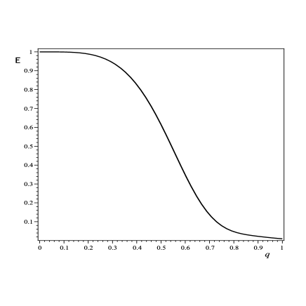
Figure 1: Plot of E for fixed $\xi$, $z$, $\tau$ and $\beta$ but varying $q$. As $q$ increases more spin decoherence occurs and so the entanglement descends.

In Fig. 1, the entanglement is sketched versus a $q$ for $\xi^{2}=0.265$, $\tau=5\tau_{0}$, $z=1.6$ and $\beta=1$. We see that by increasing the angular velocity of the centroid on the circle, E descends uniformly from 1 to an asymptotic value of zero. Such a behavior is justified because, for a constant $\tau$, by increasing $q$, the centroid travels more on its circular trajectory in the gravitational field and so more spin decoherence occurs. It is remarkable that increasing the width $\beta$, has a meaningful effect on the behavior of E in terms of $q$. This point is shown in Fig. 2 which is plotted for $\beta=4$ and the other parameters as those of Fig. 1. The entanglement again diminishes but by performing an aperiodic oscillation. This can be justified by noting that as $\beta$ increases, the exponentials in the integrals (42) and (43) approach the unity , so the cosine or sine terms play a more dominant role.

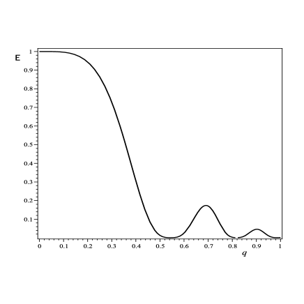
Figure 2: The same plot of figure 1 but for a larger value of $\beta$, that is a wider momentum distribution. As $q$ increases the curve again descends but by performing aperiodic oscillations.

One may also plot E in terms of $\tau/\tau_{0}$ where $\tau$ is the proper time during which the centroid moves in the gravitational field. Fig. 3 shows such a graph. Again as is expected, increasing $\tau$ produces more spin decoherence and the entanglement falls.

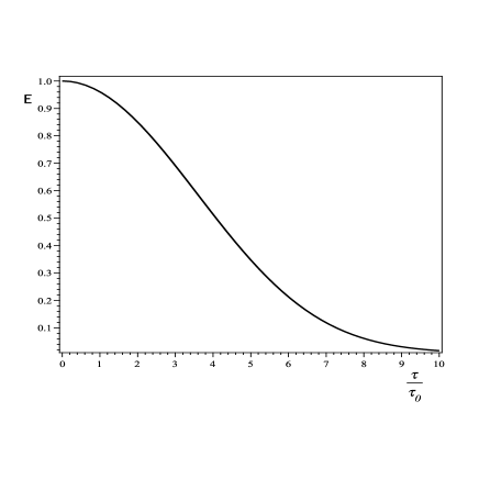
Figure 3: Plot of E for fixed $\xi$, $z$, $q$ and $\beta$ but varying $\tau$. Increasing $\tau$ also causes to occur more spin decoherence and so the entanglement diminishes.

More interesting here is to plot the entanglement in terms of the radius of the circular orbit characterized by $z$. Fig. 4 shows E versus $z$ for $\xi^{2}=0.16$, $\beta=1$, $q=0.6$ and $\tau=5\tau_{0}$. In this case there exist two horizons at $z=0.2$ and $z=0.8$, however the lower limit of $z$ is taken to be the outer horizon $z=0.8$. At any horizon $\Theta$ diverges, then the cosine and sine terms in (42), (43) oscillate rapidly yielding a zero value for the integrals. Then the entanglement (IV) is completely destroyed, leading to a fatal error in quantum communication at the horizon. On the other hand, the accessible zero of $\Theta$ occurs at $z=1.24$ where the Wigner rotation (17) becomes the identity operator. On such a circle the curvature part and the acceleration part of (4) cancel out each other, leading to a zero value for $\Theta$. Thus, for the corresponding circular orbit E remains the unity, that is, there is no decoherence for the spin Bell states. This result is independent of values of $q$, $\beta$ and $\tau$. As $z$ grows, the curve takes a minimum at $z=2.25$ which determines a circular orbit on which the effects of acceleration and curvature add to produce a maximum spin decoherence. Note that at $z\rightarrow\infty$, both the curvature part and the acceleration part of (4) vanish. Hence, as (V) shows, $\lim_{z\rightarrow\infty}\Theta=0$ and the curve asymptotically approaches to 1.

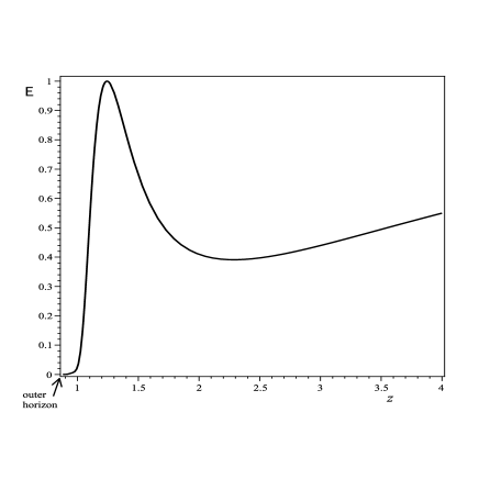
Figure 4: Plot of E for fixed $\xi$, $\tau$, $q$ and $\beta$ but varying $z$. Here $\xi$ is chosen such that there exists two event horizons for the spacetime. $z$ begins from the outer horizon where E vanishes. There is a peak which specifies the radius of a circular orbit on which no spin decoherence occurs and the entanglement remains the unity. Also, the curve takes a minimum which describes a circular orbit with maximum spin decoherence. The curve asymptotically reaches to the unity.

In the case of naked singularity $\Theta$ only diverges at $z=0$, where, the entanglement vanishes. Fig. 5 and Fig. 6 show E in terms of $z$ for this case. However, the curve in Fig. 5 is depicted for $\xi^{2}=0.265$ so $\Theta$ has two accessible zeros at $z=0.57$ and $z=0.93$ where the Wigner rotation becomes the identity operator and so the entanglement remains intact. There is no spin decoherence on these two circles, independent of the values of $q$, $\beta$ and $\tau$. Also the curve takes two minima at $z=0.65$ and $z=1.96$ indicating two circles of maximum decoherence. The curve asymptotically turns to the unity. In Fig. 6 the curve is sketched for $\xi^{2}=0.5$ and then there is no zeros for $\Theta$. By increasing $z$, the entanglement grows from zero at $z=0$ and reaches asymptotically to the unity.

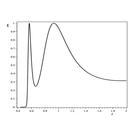
Figure 5: The same plot of figure 4 but for the case of naked singularity. In the vicinity of singularity E vanishes. $\xi$ is chosen such that $\Theta$ has two zeros at which the peak of curve occurs. The peaks designate two circles on which the entanglement remains intact. Also the curve takes two minima indicating two circles of maximum decoherence. The curve asymptotically turns to the unity.

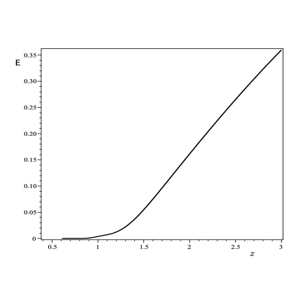
Figure 6: Plot of E versus $q$ for the case of naked singularity, but $\xi$ is chosen such that no zeros occur for $\Theta$. Then the curve grows from zero at $z=0$ and reaches asymptotically to the unity.

That on some circles E remains the unity may suggest a possibility for a perfect quantum communication around a charged black hole. The properly entangled spins of the system can preserve the stored information during the motion on such circles.

VI Frame transformation

Consider a local transformation between two instantaneously coincident inertial frames, as

$${e_{a}}^{\mu}\longrightarrow{\tilde{e}_{a}}^{\,\,\,\mu}={\mathcal{T}_{a}}^{b}(x){e_{b}}^{\mu},$$ (52)

where ${\mathcal{T}_{a}}^{c}(x){\mathcal{T}_{b}}^{d}(x)\eta_{cd}=\eta_{ab}$. Notice that the definition (1) remains intact under this tetrad transformation which can arise from a coordinate transformation $x^{\mu}\longrightarrow\tilde{x}^{\mu}$. However, as (4) implies, the new inertial observer who uses ${\tilde{e}_{a}}^{\,\,\,\mu}$ obtains different values for the components ${\lambda^{a}}_{b}(x)$, and regarding (8), we recognize that the Wigner rotation is not invariant under the transformation (52). Consequently, the spin entanglement is not frame independent. To illustrate the situation, let us simply consider the Schwarzschild black hole by letting $e^{A(r)}=e^{-B(r)}=\sqrt{1-\frac{r_{s}}{r}}$ in the metric (9). Consequently, the tetrad (11) reduces to

$${e_{0}}^{t}=\frac{1}{c\sqrt{1-\frac{r_{s}}{r}}},\,\,\,\,\,\,\,\,\,\,{e_{1}}^{r}=\frac{1}{\sqrt{1-\frac{r_{s}}{r}}},\,\,\,\,\,\,\,\,\,\,{e_{2}}^{\theta}=\frac{1}{r},\,\,\,\,\,\,\,\,\,\,{e_{3}}^{\phi}=\frac{1}{r\sin\theta},$$ (53)

which is used by a static local observer. Note that this is singular at the horizon $r=r_{s}$. Then, the local Wigner rotation elements (II) reduce to

$${w^{1}}_{3}=-{w^{3}}_{1}=c\left(\frac{1-\frac{3r_{s}}{2r}}{r\sqrt{1-\frac{r_{s}}{r}}}\right)q\sqrt{q^{2}+1}\left(\sqrt{q^{2}+1}-\frac{q\,p}{\sqrt{p^{2}+1}+1}\right),$$ (54)

which can be used for finding the elements of the Wigner rotation operator and then calculating the entanglement (IV). These elements diverge at the horizon and so the entanglement will be completely destroyed there, leading to a fatal error in quantum communication. Also they vanish at the circle $r=\frac{3r_{s}}{2}$ where the entanglement will remain intact. Now, let us transform the present spherical coordinates $(t,r,\theta,\phi)$ to, for instance, the Kruskal coordinates $(T,R,\theta,\phi)$ via the relations

$$R^{2}-c^{2}T^{2}=4r_{s}^{2}\left(\frac{r}{r_{s}}-1\right)e^{\frac{r}{r_{s}}},\,\,\,\,\,\,\,\,\,\,\,\,\,\frac{cT}{R}=\tanh\left(\frac{ct}{2r_{s}}\right).$$ (55)

In the Kruskal coordinates the Schwarzschild metric becomes

$$ds^{2}=\frac{r_{s}}{r}e^{-\frac{r}{r_{s}}}\left(-c^{2}dT^{2}+dR^{2}\right)+r^{2}\left(d{\theta}^{2}+\sin^{2}\theta\,d\phi^{2}\right),$$ (56)

where the radial coordinate $r$ is now interpreted as a function of $T$ and $R$. Accordingly, we choose a new tetrad ${\tilde{e}_{a}}^{\,\,\,\mu}$ as

$${\tilde{e}_{0}}^{\,\,\,T}=\frac{1}{c}\sqrt{\frac{r}{r_{s}}}\,e^{\frac{r}{2r_{s}}},\,\,\,\,\,\,\,\,{\tilde{e}_{1}}^{\,\,\,R}=\sqrt{\frac{r}{r_{s}}}\,e^{\frac{r}{2r_{s}}},\,\,\,\,\,\,\,{\tilde{e}_{2}}^{\,\,\,\theta}=\frac{1}{r},\,\,\,\,\,\,\,\,{\tilde{e}_{3}}^{\,\,\,\phi}=\frac{1}{r\sin\theta},$$ (57)

which is not singular at the horizon. According to (52), we find that the this tetrad is related to the static tetrad (53) by a local transformation

$${\mathcal{T}_{a}}^{c}(x)=\left(\begin{array}[]{cccc}\frac{1}{2}\sqrt{\frac{e^{-\frac{r}{r_{s}}}}{r_{s}(r-r_{s})}}\,R&-\frac{c}{2}\sqrt{\frac{e^{-\frac{r}{r_{s}}}}{r_{s}(r-r_{s})}}\,T&0&0\cr&&&\cr-\frac{c}{2}\sqrt{\frac{e^{-\frac{r}{r_{s}}}}{r_{s}(r-r_{s})}}\,T&\frac{1}{2}\sqrt{\frac{e^{-\frac{r}{r_{s}}}}{r_{s}(r-r_{s})}}\,R&0&0\cr&&&\cr 0&0&1&0\cr 0&0&0&1\end{array}\right).$$ (58)

This transformation resembles a Lorentz boost along the 1-axis and so the new local inertial observer falls into the black hole when $T>0$. Now, repeating the steps of Section 2 with the tetrad (57), we obtain, instead of (54), the local Wigner rotation elements

$${\tilde{w}^{1}}_{\,\,\,3}=-{\tilde{w}^{3}}_{\,\,\,1}=\frac{c}{4r}\sqrt{\frac{e^{-\frac{r}{r_{s}}}}{rr_{s}}}\left(3+\frac{r}{r_{s}}\right)\tilde{q}\sqrt{\tilde{q}^{2}+1}\left(\sqrt{\tilde{q}^{2}+1}-\frac{\tilde{q}\,\tilde{p}}{\sqrt{\tilde{p}^{2}+1}+1}\right),$$ (59)

where $\tilde{q}$ and $\tilde{p}$ relate to the four-momentum of the centroid and the four-momentum of particles, respectively, that are chosen by the falling observer. Since these elements are not singular at the horizon, the spin entanglement can have a nonzero value and falling observers just on the horizon can perform a quantum information task with a finite error. Furthermore, they can do this beyond the horizon $r<r_{s}$, until the physical singularity $r=0$. Therefore, the features of quantum communication in a curved spacetime using the entangled spins depend on the tetrad that is used by the observer.

VII Conclusion

In this paper we discussed the effect of a gravitational field on the spin entanglement of a system of two spin-$\frac{1}{2}$ particles moving in the gravitational field. We described the system by a two-particle Gaussian wave packet represented in the momentum space with a definite width around the momentum of a mean centroid. We considered the mean centroid for describing the motion of the system in the gravitational field which was a classic field in our approach. Both the acceleration of the centroid and the curvature of the gravitational field caused to produce a Wigner rotation acting on the wave packet. We confined the argument to spherically symmetric and static gravitational field such as a charged black hole. At a given initial point in the curved spacetime, the momenta of the particles were taken to be separable, while the spin part was chosen to be entangled as the Bell states. By calculating the reduced density operator, we focused on the spin entanglement of the system.

For any spherically symmetric and static spacetime, when the system, no matter of spin and momentum entanglements, falls along a radial geodesic, the Wigner rotation is trivial and so the spin density matrix remains intact. Moreover, for a charged black hole, depending on the mass and the charge of black hole, there can be circular paths with determined radii on which the spin entanglement is invariant. For instance, it always remains the unity, provided spins be entangled initially as one of the Bell states. This result is a consequence of cancellation of the acceleration and the curvature on such circles. The spin entanglement descends to zero by increasing the angular velocity of the centroid as well increasing the proper time during which the centroid moves on its circular path around the center of charged black hole.

It is remarkable that the features of quantum communication in a curved spacetime using the entangled spins depend on the tetrad that is used by the observer.

As an extension of this work, one can provide the initial state with a specified spin entanglement and also a specified momentum entanglement, then discuss the final spin entanglement, as well as the final momentum entanglement.

References

• (1) A. Peres, P. F. Scudo, and D. R. Terno. Phys. Rev. Lett., 88:230402, 2002.
• (2) H. Terashima and M. Ueda. Quantum Inf. Comput, 3:224, 2003.
• (3) P. M. Alsing and G. J. Milborn. Quantum Inf. Comput., 2:487, 2002.
• (4) D. Ahn, H. J. Lee, Y. H. Moon, and S. W. Hwang. Phys. Rev. A, 67:012103, 2003.
• (5) D. Lee and C. Y. Ee. New J. Phys., 6:67, 2004.
• (6) W. T. Kim and E. J. Son. Phys. Rev. A, 71:014102, 2005.
• (7) R. M. Gingrich and C. Adami. Phys. Rev. Lett., 89:270402, 2002.
• (8) H. Li and J. Du. Phys. Rev., A68:022108, 2003.
• (9) P. M. Alsing, I. Fuentes-Schuller, R. B. Mann, and T. E. Tessier. Phys. Rev., A74:032326–1, 2006.
• (10) Q. Pan and J. Jing. Phys. Rev., A77:024302–1, 2008.
• (11) X. H. Ge and Y. G. Shen. Phys. Lett., B606:184, 2005.
• (12) X. H. Ge and S. P. Kim. Class. Quantum Gravit., 25:1–20, 2008.
• (13) H. Terashima and M. Ueda. J. Phys., A38:2029, 2005.
• (14) B. Nasr and S. Dehdashti. Int. J. Theor. Phys, 46:1495, 2007.
• (15) R. D’Inverno. Introducing Einstein’s Relativity. Oxford University press, Oxford, 1992.
• (16) H. Terashima and M. Ueda. Phys. Rev., A69:032113, 2004.
• (17) S. Weinberg. The Quantum Theory of Fields. Cambridge University press, Cambridge, 1995.
• (18) W. K. Wootters. Phys. Rev. Lett, 80:2245, 1998.