Modified gravity in a viscous and non-isotropic background

Abstract

We study the dynamical evolution of an $f(R)$ model of gravity in a viscous and anisotropic background which is given by a Bianchi type-I model of the Universe. We find viable forms of $f(R)$ gravity in which one is exactly the Einsteinian model of gravity with a cosmological constant and other two are power law $f(R)$ models. We show that these two power law models are stable with a suitable choice of parameters. We also examine three potentials which exhibit the potential effect of $f(R)$ models in the context of scalar tensor theory. By solving different aspects of the model and finding the physical quantities in the Jordan frame, we show that the equation of state parameter satisfy the dominant energy condition. At last we show that the two power law $f(R)$ models behave like quintessence model at late times and also the shear coefficient viscosity tends to zero at late times.

1 Introduction

Observational data (Riess et al., 1998; Perlmutter et al, 1999; Spergel et al., 2003; Tegmark et al., 2004) indicates several shortcoming in the standard model of gravity (SGR) (Wald, 1984; Weinberge, 1984; Misner et al., 1970). These shortcoming are related to cosmology, large scale structure and quantum field theory. These problems have spanned several theoretical models. For example: the quintessence scenario, which generalizes the cosmological constant approach (Caldwell at al., 1998; Sahni and Starobinsky, 2000); higher dimensional scenarios (Maartens, 2004; Pietroni, 2003; Nozari and Rashidi, 2010); or the resort to cosmological fluids with exotic equations of state (Bento at al., 2003; Nojiri and Odintsov, 2007; Nojiri and Odinsov, 2005). Another interesting approach is $f(R)$ gravity, which generalizes the geometrical part of the Hilbert-Einstein Lagrangian (Capozziello, 2002; Carroll at al., 2004; Carroll et al., 2005; Nojiri and Odintsov, 2003; Clifton and Barrow, 2005; Nojiri and Odintsov, 2006; Aghmohammadi et al., 2010, 2011, 2009; Saaidi and Aghmohammadi, 2011; Karami and Fehri, 2010; Karami et al., 2010; Amendola et al., 2007; Amendola et al, 2007; Nojiri and Odintsov, 2007; Capozziello et al., 2006, 2008; Capozziello and Stabile, 2009; Nojiri et al., 2005; Nozari and Azizi, 2009).

The isotropy of the cosmic microwave background (CMB) radiation was first reported by the cosmic background explorer (COBE) satellite (Smoot et al., 1992), and subsequently reinforced by the Wilkinson Microwave Anisotropy Probe (WMAP) data (Hinshaw et al., 2003). These observations, coupled with the assumption that we cannot be in a special position in the universe, imply that we live in a homogeneous and isotropic Universe described by a Friedmann-Lema$\hat{\rm i}$tre-Robertson-Walker (FLRW) line-element. For this reason, nearly all research on the dynamical evolution of the Universe is done in the homogenous and isotropic space-time background.

On the other hand, although the Universe seems isotropic and homogeneous at present, the large scale matter distribution in the observable Universe, largely manifested in the form of discrete structures, does not show homogeneity of a higher order. Moreover, according to a statistical analysis of 4-yr data from the COBE satellite, tiny deviation from isotropy at the level of $10^{-5}$ has been suggested by (Bunnett et al., 1996), and this suggestion was confirmed by high resolution WMAP data. These studies, which support the existence of anisotropic phase, lead us to consider the dynamical evolution of the Universe with an anisotropic background.

A Bianchi type-I (BI) Universe, being the straightforward generalization of the flat FLRW Universe, is of interest because it is one of the simplest models of a non-isotropic Universe exhibiting a homogeneity and spatial flatness. In this case, unlike the FLRW Universe which has the same scale factor for three spatial directions, a BI Universe has a different scale factor for each direction. This fact introduce a non-isotropy to the system. The possible effects of anisotropy in the early Universe have been investigated with Bianchi I type models from different points of view (Komatsu et al, 2009; Kumar et al, 2011; Yadav et al., 2011; Yadav, 2011; Saha, 2001; Saha and Boyadjiev, 2004; Khalatnikov and kamenshchik, 2003). Some other papers dealing with anisotropic cosmology are (Bertschinger, 1994; Guzman, 1993; Halpern, 1994; Van den Hoogen, 1995; Kalligas et al., 1995; Brevik and Pettersen, 1997; Caderni and Fabbri, 1977) but, to the best of our knowledge, there are no detailed studies of $f(R)$ gravity in an anisotropic background. Therefore, we investigate the dynamical evolution of the Universe with a viscous and anisotropic background in $f(R)$ gravity.

The present paper is organized as follows: In Sec. 2, we review $f(R)$ model and the conformal transformation between the Jordan frame and the Einstein frame. In Sec. 3, we consider the field equations of $f(R)$ gravity in a non-isotropic space-time. Sec. 4, considers the set of solutions to the field equations. Finally, the latter section is devoted to conclusions.

2 Preliminary

We study the Bianchi type I (BI) cosmological model as a gravitational field in modified gravity. The BI model is the simplest model of a non-isotropic Universe that describes a homogeneous and spatially flat space-time.

2.1 $f(R)$ gravity

We consider the general form of the action for $f(R)$ gravity to be given by

$$S_{f(R)}=\int d^{4}x\sqrt{-g}\left[\frac{f(R)}{2}+\kappa{L}_{m}(g_{\mu\nu,\psi})\right],$$ (1)

where $f(R)$ is a function of the Ricci scalar $R$, $g_{\mu\nu}$ is the metric of space-time, $\psi$ is the matter field, and ${L}_{m}(g_{\mu\nu},\psi)$ is the matter Lagrangian. We assume the metric $g_{\mu\nu}$ is the only independent variable. Taking the variation of (1) with respect to $g_{\mu\nu}$ gives

$$R_{\mu\nu}f^{\prime}(R)-\frac{1}{2}f(R)g_{\mu\nu}-\nabla_{\mu}\nabla_{\nu}f^{\prime}(R)+g_{\mu\nu}\square f^{\prime}(R)=T^{m}_{\mu\nu},$$ (2)

where $T^{m}_{\mu\nu}$, the stress-energy tensor of matter, is defined by

$$T^{m}_{\mu\nu}=-\frac{2}{\sqrt{-g}}\frac{\delta(\sqrt{-g}{L}_{m})}{\delta g^{\mu\nu}}.$$ (3)

We have taken $\kappa=1$ in this work.

2.2 Conformal transformation

As regards $f(R)$ model of gravity can be rewritten as scalar tensor theories via a famous conformal transformation:

$$e^{-2\beta\phi}=f^{\prime}(R).$$ (4)

Using Eq. (4), one can rewrite Eq. (1) as

$$S_{ST} = \int d^{4}x\sqrt{-\bar{g}}\Bigg{[}\frac{\bar{R}}{2}-\frac{1}{2}\bar{g}^{\mu\nu}\nabla_{\mu}\phi\nabla_{\nu}\phi-V(\phi)$$

$$\;\;\;\;\;\;\;\;\;\;\;\;\;\;\;\;\;\;\;\;\;\;\;+{L}_{m}(e^{2\beta\phi}\overline{g}_{\mu\nu},\psi)\Bigg{]},$$

where we have defined the Einstein frame metric, $\bar{g}_{\mu\nu}$, by a conformal transformation $\bar{g}_{\mu\nu}=e^{-2\beta\phi}g_{\mu\nu}$. The potential $V(\phi)$ is given by

$$V(\phi)=\frac{Rf^{\prime}(R)-f(R)}{2f^{\prime}(R)^{2}}.$$ (6)

Variation of Eq. (2.2) with respect to $\bar{g}_{\mu\nu}$ and $\phi$ gives

$$\bar{R}_{\mu\nu}-\frac{1}{2}\bar{R}\bar{g}_{\mu\nu}=\nabla_{\mu}\phi\nabla_{\nu}\phi+\bar{g}_{\mu\nu}\biggr{[}\frac{1}{2}(\nabla\phi)^{2}+V(\phi)\biggl{]}+\bar{T}_{\mu\nu}^{m},$$ (7)

and

$$\bar{\square}\phi=V^{\prime}(\phi)-\beta\bar{T}^{m},$$ (8)

where $\bar{\nabla}_{\mu}\bar{g}_{\mu\nu}=0$ is used. Note that in the Einstein frame all indices are lowered and raised by $\bar{g}_{\mu\nu}$.

The line element of the BI type can be expressed as

$$ds^{2}=dt^{2}-A^{2}(t)dx^{2}-B^{2}(t)dy^{2}-C^{2}(t)dz^{2},$$ (9)

where the metric function, $A,B,C$, are functions of time, $t$, only. This model is an anisotropic generalization of the Friedmann model with Euclidean spatial geometry. The expansion factors, $A$, $B$, $C$, are determined via Einstein’s equation. In this work, we shall restrict ourselves to the Kasner form of the metric as:

$$ds^{2}=dt^{2}-t^{2p_{1}}dx^{2}-t^{2p_{2}}dy^{2}-t^{2p_{3}}dz^{2},$$ (10)

where $p_{1}$, $p_{2}$, $p_{3}$ are three parameters which we will require to be constant. The space is anisotropic if $p_{i}\neq p_{j},(i,j=1,2,3)$.

3 Field equations

By making use of Eqs. (7) and (8), we can derive the field equations. Using Eq. (10) and introducing symbols $S\equiv p_{1}+p_{2}+p_{3}$ and $Q\equiv p_{1}^{2}+p_{2}^{2}+p_{3}^{2}$, the components of Ricci tensor, namely $\bar{R}_{00}$ and $\bar{R}_{ii}$ are

$$\bar{R}_{00}=\frac{S-Q}{t^{2}}+\frac{S\beta\dot{\phi}}{t}+3\beta\ddot{\phi},$$ (11)

$$\bar{R}_{ii}=t^{2p_{i}}\left[\frac{p_{i}(S-1)}{t^{2}}-\frac{\beta\dot{\phi}}{t}(S+2p_{i})+2\beta^{2}\dot{\phi^{2}}-\beta\ddot{\phi}\right].$$ (12)

We consider the stress-energy momentum tensor for a viscous fluid:

$$T_{\mu\nu}=\left[\rho+(P-\xi\theta)\right]u_{\mu}u_{\nu}-(P-\xi\theta)g_{\mu\nu}+2\eta\sigma_{\mu\nu},$$ (13)

where $u_{\mu}$, $\rho$, $P$, $\xi$ and $\eta$ are the fluid’s four velocity, energy density, isotropic pressure, bulk and shear viscosities, respectively. The scalar expansion and traceless shear tensors are

$$\theta_{\mu\nu}=\frac{1}{2}\left[u_{\mu;\alpha}h^{\alpha}_{\nu}+u_{\nu;\alpha}h^{\alpha}_{\mu}\right],$$ (14)

$$\sigma_{\mu\nu}=\theta_{\mu\nu}-\frac{1}{3}h_{\mu\nu}\theta,$$ (15)

respectively. Here, $h_{\mu\nu}=u_{\mu}u_{\nu}-g_{\mu\nu}$ is the projection operator. Taking the trace of Eq.(7) gives :

$$\bar{R}=(\bar{\nabla}\phi)^{2}+4V(\phi)-\bar{T}^{m}.$$ (16)

By substituting Eq. (16) into Eq. (7), we have

$$\bar{R}_{\mu\nu}=e^{2\beta\phi}\big{[}T_{\mu\nu}-\frac{1}{2}Tg_{\mu\nu}\big{]}+e^{-2\beta\phi}g_{\mu\nu}V(\phi)+\nabla_{\mu}\phi\nabla_{\nu}\phi.$$ (17)

So the components $\bar{R}_{00}$, $\bar{R}_{ii}$ are

$$\bar{R}_{00}=e^{2\beta\phi}\biggr{[}\rho-\frac{1}{2}\big{\{}\rho-3(P-\xi\theta)\big{\}}\biggl{]}+e^{-2\beta\phi}V(\phi)+\dot{\phi}^{2},$$ (18)

$$\bar{R}_{ii} = \bigg{[}\frac{e^{2\beta\phi}}{2}\left\{\rho-(P-\xi\theta)+\frac{4\eta}{t}(\frac{S}{3}-p_{i})\right\}$$

$$\;\;\;\;\;\;\;\;\;\;-e^{-2\beta\phi}V(\phi)\bigg{]}t^{2p_{i}}.$$

Using Eqs. (11), (12), (18) and (3), one can gets that

$$e^{2\beta\phi}\bigg{[}\rho-\frac{1}{2}\big{\{}\rho-3(P-\xi\theta)\big{\}}\bigg{]}+e^{-2\beta\phi}V(\phi)+\dot{\phi}^{2}$$

$$\;\;\;\;\;\;\;\;\;\;\;\;\;\;=\frac{S-Q}{t^{2}}+\frac{S\beta\dot{\phi}}{t}+3\beta\ddot{\phi},$$ (20)

$$p_{i}\bigg{[}{-2\eta}{t}e^{2\beta\phi}+\frac{(1-S)}{t^{2}}+\frac{2\beta\dot{\phi}}{t}\bigg{]}+\frac{S\beta\dot{\phi}}{t}-2\beta^{2}\dot{\phi^{2}}+\beta\ddot{\phi}$$

$$\;\;\;\;\;=-\frac{e^{2\beta\phi}}{2}\left[\rho-(P-\xi\theta)+\frac{4\eta S}{3t}\right]+e^{-2\beta\phi}V(\phi).$$ (21)

Since the $p_{i}{\rm s}$ $(i=1,2,3)$ are linearly independent, we find that

$$\eta=\big{[}\frac{1-S}{2t}+\beta\dot{\phi}\big{]}e^{-2\beta\phi}.$$ (22)

Substituting Eq. (22) into the right hand side of Eq. (21) gives

$$e^{2\beta\phi}\Big{[}\rho-(P-\xi\theta)\Big{]}=4\beta^{2}\dot{\phi}^{2}-2\beta\ddot{\phi}$$ (23)

$$\;\;\;\;\;\;\;-\frac{10}{3}\frac{S\beta\dot{\phi}}{t}-\frac{2S(1-S)}{3t^{2}}+2e^{-2\beta\phi}V(\phi).$$

By combining Eqs. (23) and (20), we obtain explicit expression for $\rho$ and $p$ as follows

$$e^{2\beta\phi}(P-\xi\theta) = \frac{1}{6t^{2}}\left[4S-3Q-{S^{2}}\right]+\frac{4}{3}\frac{S\beta}{t}\dot{\phi}$$

$$\;\;\;\;\;+2\beta\ddot{\phi}-[\beta^{2}+\frac{1}{2}]\dot{\phi}^{2}-e^{-2\beta\phi}V(\phi),$$

$$e^{2\beta\phi}\rho=\frac{1}{2t^{2}}(S^{2}-Q)+e^{-2\beta\phi}V(\phi)-2\beta\frac{S}{t}\dot{\phi}+(3\beta^{2}-\frac{1}{2})\dot{\phi}^{2}.$$ (25)

Substituting Eqs. (3) and (25) into Eq. (8), we get that the equations of motion for the scalar field $\phi$, are

$$\ddot{\phi}+\dot{\phi}\frac{S}{t}-\beta\dot{\phi}^{2}=\frac{e^{-2\beta\phi}}{(1-6\beta^{2})}\left[V^{\prime}(\phi)-4\beta V(\phi)\right]+\frac{C}{t^{2}},$$ (26)

where

$$C=\frac{\beta}{(1-6\beta^{2})}\left(2S-S^{2}-Q\right).$$

4 The solutions

In this section we want to solve Eq. (26). As an ansatz, we suggest

$$\phi=\phi_{0}\ln(t),$$ (27)

where $\phi_{0}$ is a constant with the same dimension as $\phi$ and $t$ is a dimensionless time parameter such as $t={\tau/\tau_{0}}$, where $\tau_{0}$ can be the present time. By this choice, we can consider three classes of solution as follows.

4.1 Case I

A class of solutions to Eq. (26) is given by

$$\frac{e^{-2\beta\phi}}{(1-6\beta^{2})}\Big{[}V^{\prime}(\phi)-4\beta V(\phi)\Big{]}=0,$$ (28)

$$\ddot{\phi}+\dot{\phi}\frac{S}{t}-\beta\dot{\phi}^{2}-\frac{C}{t^{2}}=0.$$ (29)

In this case we assume $\phi=\phi_{1}\ln(t)$, where $\phi_{1}$ is a constant. Solving Eq. (28), gives

$$V(\phi)=V_{1}e^{4\beta\phi},$$ (30)

where $V_{1}$ is an integration constant. By substituting Eq. (30) into Eq. (29), we obtain the following constraint:

$$(S-1)\phi_{1}-\beta\phi_{1}^{2}-C=0.$$ (31)

Also, we can find that $\rho$, $P$ and $\eta$ are

$$\rho=V_{1}+\frac{\rho_{1}}{t^{2\alpha_{1}}},$$ (32)

$$P=-V_{1}+\frac{S}{t}\xi+\frac{P_{1}}{t^{2\alpha_{1}}},$$ (33)

and

$$\eta=\left[{1-S}+2\beta\phi_{1}\right]\frac{1}{2t^{2\alpha_{1}-1}}.$$ (34)

Where

$$\rho_{1}={1\over 2}\bigg{[}{S^{2}-Q}+\biggr{\{}(6\beta^{2}-1)\phi_{1}-2\beta S\biggl{\}}\phi_{1}\bigg{]},$$ (35)

$$P_{1}={1\over 6}\bigg{[}4S-3Q-S^{2}+\left\{8S\beta-12\beta-(6\beta^{2}+3)\phi_{1}\right\}\phi_{1}\bigg{]},$$ (36)

and

$$\alpha_{1}=(\beta\phi_{1}+1).$$

From Eqs. (32) and (33) we can find the equation of state parameter, $\gamma=P/\rho$ as

$$\gamma={P\over\rho}=-1+{(\gamma_{1}+1)\rho_{1}\over V_{1}t^{2\alpha_{1}}+\rho_{1}}+{S\xi\over V_{0}t+{\rho_{0}\over t^{2\alpha_{1}}-1}},$$ (37)

here $\gamma_{1}=P_{1}/\rho_{1}$.

Using Eqs. (30) and (6), one can obtain that the viable $f(R)$ and $V(R)$ function are

$$f(R) = -2V_{1}+f_{1}R,$$ (38)

$$V(R) = {V_{1}\over f_{1}^{2}}$$ (39)

where $f_{1}$ is an integration constant and $2V_{1}$ is similar to the cosmological constant $\Lambda$. In this case, the $f(R)$ model of gravity is exactly the standard Einsteinian model of gravity.

4.2 Case II

We assume $\phi=\phi_{2}\ln(t)$, where $\phi_{2}$ is a constant. So, we suggest another class of solutions which satisfy the following equations:

$$\frac{e^{-2\beta\phi}}{(1-6\beta^{2})}\Big{[}V^{\prime}(\phi)-4\beta V(\phi)\Big{]} = \frac{B}{t^{2}},$$ (40)

$$\ddot{\phi}+\dot{\phi}\frac{S}{t}-\beta\dot{\phi}^{2}-\frac{B+C}{t^{2}} = 0,$$ (41)

where $B$ is a constant. From Eq. (40), we have

$$V(t)=V_{2}t^{2\beta\phi_{2}-2},$$ (42)

where

$$V_{2}=\frac{B(6\beta^{2}-1)\phi_{2}}{2(1+\beta\phi_{2})}.$$ (43)

By substituting Eq. (42) into Eq. (41), we can obtain a constraint which $\phi_{2}$ has to satisfy:

$$(S-1)\phi_{2}-\beta\phi_{2}^{2}-B-C=0.$$ (44)

Also, we get that $\rho$, $P$ and $\eta$ are

$$\rho = {\rho_{2}\over t^{2(\beta\phi_{2}+1)}}+V_{0}t^{2(\beta\phi_{2}-1)},$$ (45)

$$P = {P_{2}\over t^{2(\beta\phi_{2}+1)}}-V_{0}t^{2(\beta\phi_{2}-1)}+\frac{S}{t}\xi,$$ (46)

$$\eta = {1\over 2}\left[1-S+2\beta\phi_{2}\right]\frac{1}{t^{(2\beta\phi_{2}+1)}}.$$ (47)

where

$$\rho_{2}={1\over 2}\left[{S^{2}-Q}+(6\beta^{2}-1)\phi_{2}^{2}-4\beta S\phi_{2}\right],$$ (48)

and

$$P_{2}={1\over 6}\bigg{[}(8S\beta-12\beta)\phi_{2}-(6\beta^{2}+3)\phi_{2}^{2}+4S-3Q-S^{2}\bigg{]}.$$ (49)

From Eqs. (45 ) and (46) we have

$$\gamma={P\over\rho}=-1+{P_{2}+\rho_{2}+S\xi t^{(2\beta\phi_{2}-1)}\over\rho_{2}+V_{0}t^{4\beta\phi_{2}}}.$$ (50)

Using Eqs. (42) and (6), we get that the viable $f(R)$ and $V(R)$ functions are:

$$f(R) = f_{2}R^{1-\epsilon},$$ (51)

$$V(R) = -{\epsilon\over 2(1-\epsilon)^{2}f_{2}}R^{1+\epsilon},$$ (52)

$$V(\phi) = -{\epsilon\big{[}(1-\epsilon)f_{2}\big{]}^{1\over\epsilon}\over 2(1-\epsilon)^{2}f_{2}}e^{{2\beta(1+\epsilon)\over\epsilon}\phi},$$ (53)

where $f_{2}$ is the constant of integration and

$$\epsilon={B\phi_{2}\over B\phi_{2}+S^{2}+Q-4S}.$$ (54)

To obtain stability for the above $f(R)$, the following condition must be satisfied (Aghmohammadi et al., 2009):

$$\frac{d^{2}f}{dR^{2}}>0.$$ (55)

One can see that Eq. (51) is stable when

$$\epsilon<0.$$ (56)

From Eqs. (51) and (60), one can see that for $\beta\phi_{2}=0(\epsilon=0)$, it follows that $f(R)=R$, which is the standard Einsteinian model of gravity. However, for $\beta\phi_{2}=0(\epsilon=0)$, the quantities $\rho$, $P$ and $\eta$ are:

$$\rho=\frac{S^{2}-Q}{2t^{2}},$$ (57)

$$P-\frac{S}{t}\xi=\dfrac{4S-S^{2}-3Q}{6t^{2}},$$ (58)

$$\eta=\frac{1-S}{2t}.$$ (59)

These results are in (Brevik and Pettersen, 1997). The dominant energy condition (DEC) requires $-\rho+\frac{S}{t}\xi\leq P\leq\rho+\frac{S}{t}\xi$. Then, from Eqs. (57), (58) and (59), for $P\leq\rho+\frac{S}{t}\xi$, we have that $1\leq S$. For the case $-\rho+\frac{S}{t}\xi\leq P$, we obtain $S(S+2)\geq 3Q$. Thus, from these expressions it is easy to see that $\eta\leq 0$ and $\rho\geq 0$.

4.3 Case III

In this case we assume $\phi=\phi_{3}\ln(t)$ and $B=-C$. According to Eq. (44) $\phi_{3}$ is

$$\phi_{3}={S-1\over\beta},$$ (60)

and Eq. (42) reduces to

$$V(t)=V_{3}t^{2(S-2)},$$ (61)

where

$$V_{3}=\frac{(2S-S^{2}-Q)(S-1)}{2S}.$$

We can obtain physical quantities as

$$\rho = {\rho_{2}\over t^{2S}}+V_{3}t^{2(S-2)},$$ (62)

$$P = {P_{2}\over t^{2S}}+\frac{S}{t}\xi-V_{3}t^{2(S-2)},$$ (63)

$$\eta = \frac{(S-1)}{2t^{2S-1}}.$$ (64)

Here

$$\rho_{3}={1\over 2}\left[{3S^{2}-Q}-8S+6-\frac{(S-1)^{2}}{\beta^{2}}\right],$$ (65)

$$P_{3} = {1\over 6}\bigg{[}S^{2}-4S+6-3Q-\frac{3(S-1)^{2}}{\beta^{2}}\bigg{]},$$ (66)

and we can obtain $f(R)$ and $V(R)$ as

$$f(R) = f_{3}R^{1+\epsilon},$$ (67)

$$V(R) = \Big{[}{W-2V_{3}\over 2Wf_{3}}\Big{]}R^{1-\epsilon},$$ (68)

$$V(\phi) = \Big{[}{W-2V_{3}\over 2W^{\epsilon}f_{3}}\Big{]}e^{{2\beta(1-\epsilon)\over S-1}\phi},$$ (69)

where $f_{3}$ is an integration constant and

$$\epsilon={2V_{3}\over W-2V_{3}},\hskip 42.67912ptW={1\over 4}(4S-S^{2}-Q).$$ (70)

One can show that this model is stable if $\epsilon>0$.

Since the shear coefficient of viscosity at early time is much bigger than the bulk viscosity (Caderni and Fabbri, 1977), we take $\xi=0$. Moreover, for simplicity we suppose a special non-isotropic background given by $p_{1}=p_{2}=p$ and $p_{3}=np$, where $n$ is a positive constant. However, one can write the barotropic equation of state as $P=\gamma\rho$. It is well known that the dominant energy condition (DEC) imply that $\gamma$ lies in the interval [-1, 1]. From Eqs. (62) and (63), and the above assumptions, we can obtain the equation of state parameter as

$$\gamma=-1+{P_{3}+\rho_{3}\over\rho_{3}+V_{3}t^{4(S-1)}}.$$ (71)

In order to gain better insight we make a suitable choice of parameters. For example, we let $p=0.45$, $n=1.2$ and $\beta=\sqrt{2/3}$. For this choice, $S=1.44$ and $\epsilon\approx 0.047$, which means that the model is stable. We plot the equation of state parameter $\gamma$ and the shear coefficient of viscosity $\eta$ versus $t$ if Fig. 1. Fig. 1a indicates that the equation of state parameter belongs to $[-1,1]$. I.e., this model can satisfy the DEC, and by increasing time it is saturated to $-1$. This means our model behave like a quintessence model at late times. Fig. 1b shows that the shear coefficient of viscosity is notable at early times and as time passes it tends to zero. Namely, the part of viscosity coming from the non-isotropic form of background is negligible at late times ( the present time).

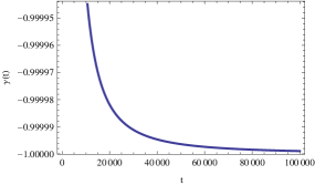
(a)

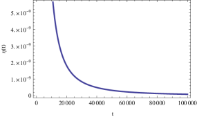
(b)

Fig. 1 : (a): This sub-figure shows the equation of state parameter, $\gamma$, versus cosmic time. (b): This sub-figure shows the shear coefficient viscosity, $\eta$, versus cosmic time, $t$. We have taken $p=0.45$, $n=1.2$ and $\beta=\sqrt{2/3}$.

5 Conclusion

The main purpose of the present work is to study $f(R)$ gravity in an anisotropic metric, such as the Kasner metric. We have assumed that the Universe is filled by a viscous cosmic fluid which is endowed with a shear viscosity $\eta$ and a bulk viscosity $\xi$. In this work, we have obtained three viable forms of $f(R)$ gravity in which one was exactly the Einsteinian model of gravity with a cosmological constant and the other two were power law $f(R)$ models. We showed that these two power law modified models of gravity are stable with a suitable choice of parameters. Also, we solved different aspects of the model and found physical quantities in the Jordan frame. Our study shows that the equation of state parameter satisfies the dominant energy condition. Moreover, the power law $f(R)$ models behave like a quintessence model at late times and the shear coefficient viscosity tends to zero at late times.

6 Acknowledgement

The authors thank the referee for illuminating remarks that enabled them to improve the clarity of this paper and also the authors would like thank to S. Westmoreland for assisting for clarity the English in this paper.

References

• Aghmohammadi et al. (2010) Aghmohammadi, A., Saaidi, K., Abolhassani., M.R.: Int. J. Theor Phys. 49, 709 (2010)
• Aghmohammadi et al. (2011) Aghmohammadi, A., Saaidi, K.: Phys. Scr. 83, 025902 (2011)
• Aghmohammadi et al. (2009) Aghmohammadi, A., Abolhassani, M. R., Vajdi, A., Phys. Scripta 80, 065008 (2009)
• Amendola et al. (2007) Amendola, L., et al.: Phys. Rev. D 75, 083504 (2007)
• Amendola et al (2007) Amendola, L., et al.: Phys. Rev.Lett. 98, 131302 (2007) Amirhashchi, H., Pradhan, A. and Saha , B.: 333, 295 (2011)
• Bento at al. (2003) Bento, M. C.: Bertolami, O. Sen, A. A. Phys. Rev. D 67, 063003 (2003)
• Bertschinger (1994) Bertschinger, E.: Physica D 77, 354 (1994)
• Brevik and Pettersen (1997) Brevik, I., Pettersen, S. V.: Phys. Rev. D 56, 3322 (1997)
• Bunnett et al. (1996) Bunnett, E. F., Ferreira, P. G. and Silk, J.: Phys. Rev. Lett. 77, 2883 (1996)
• Guzman (1993) Guzman, E.: Astrophys. Space Sci. 199, 289 (1993)
• Caderni and Fabbri (1977) Caderni, N. and Fabbri, R.: Phys. Lett. B 69, 508 (1977)
• Capozziello et al. (2006) Capozziello, S., et al.: Phys. lett. B 639, 135 (2006)
• Capozziello et al. (2008) Capozziello, S., et al.: Class. Quant. Grav. 25, 085004 (2008)
• Capozziello and Stabile (2009) Capozziello, S., Stabile, A.: Class. Quant. Grav. 26, 085019 (2009)
• Capozziello (2002) Capozziello, S.: Int. J. Mod. Phys. D 11, 483 (2002)
• Caldwell at al. (1998) Caldwell, R.R., Dave, R. Steinhardt, P.J.: Phys. Rev. Lett. 80, 1582 (1998)
• Carroll at al. (2004) Carroll, S.M., Duvvuri, V., Trodden, M., Turner, M.S.: Phys. Rev. D 70, 043528 (2004)
• Carroll et al. (2005) Carroll, S.M., et al.: Phys. Rev. D 71, 063513 (2005)
• Clifton and Barrow (2005) Clifton, T., Barrow, J.D.: Phys. Rev. D 72, 103005 (2005)
• Halpern (1994) Halpern, P.: Gen. Relativ. Gravit. 26, 781 (1994)
• Hinshaw et al. (2003) Hinshaw et al. : Astrophys. J. Suppl. 148, 135 (2003)
• Kalligas et al. (1995) Kalligas, D., Wesson, P.S. and Everitt, C.W.F.: Gen. Relativ. Gravit. 27, 645 (1995)
• Khalatnikov and kamenshchik (2003) Khalatnikov, I.M. and kamenshchik, A.Yu.: Phys. Lett. B 553, 119 (2003)
• Karami and Fehri (2010) Karami, K., Fehri, J.: Int. J. Theor. Phys. 49, 1118 (2010)
• Karami et al. (2010) Karami, K., Khaledian, M.S., Felegary, F., Azarmi, Z.: Phys. Lett. B 686, 216 (2010)
• Komatsu et al (2009) Komatsu, E. et al: Astrophys. J. Suppl. Ser. 180, 330 (2009)
• Kumar et al (2011) Kumar, S. and Yadav, A. K.: Mod. Phys. Lett. A 26, 647 (2011)
• Misner et al. (1970) Misner, C. W. Thorne, K.S. and Wheeler, J.A.: Gravitation (San Francisco: W. H. Freeman and company) (1970)
• Maartens (2004) Maartens, R.: Living Rev. Rel. 7, 7 (2004)
• Nojiri and Odinsov (2005) Nojiri, S., and Odintsov, S.D.: Phys. Rev. D 72, 023003 (2005)
• Nojiri and Odintsov (2007) Nojiri, S., and Odintsov: Int. J. Geom. Meth. Mod. Phys. 4 115 (2007)
• Nojiri et al. (2005) Nojiri, S., Odintsov, S. D., and Tsujikawa, S., Phys. Rev. D 71, 063004 (2005)
• Nojiri and Odintsov (2003) Nojiri, S. Odintsov, S. D., Phys. Rev. D 68, 123512 (2003)
• Nojiri and Odintsov (2006) Nojiri, S. Odintsov, S.D.: Phys. Rev. D 74, 086005 (2006): Phys. Lett. B 657, 238 (2007)
• Nojiri and Odintsov (2007) Nojiri, S. Odintsov, S. D.: arxiv:0710.1738; V. Faraoni,: Phys. Rev. D 74, 104017 (2006); I. Sawicki, W. Hu,: Phys. Rev. D 75, 127502 (2007)
• Nozari and Rashidi (2010) Nozari, K. and Rashidi, N.: Int. J. Mod. Phys. D 19, 219 (2010)
• Nozari and Azizi (2009) Nozari, K. and Azizi, N,: Phys. Lett. B 680, 205 (2009)
• Perlmutter et al (1999) Perlmutter, S. et al.: Astrophys. J. 517, 565 (1999)
• Pietroni (2003) Pietroni, M. Phys. Rev. D67, 103523 (2003)
• Riess et al. (1998) Riess, A. G. et al.: L. 116, 1009 (1998)
• Saaidi and Aghmohammadi (2011) Saaidi, Kh., and Aghmohammadi, A.,: Astrophys. Space Sci. 333, 327 (2011)
• Sahni and Starobinsky (2000) Sahni, V. and Starobinsky, A. A.: Int. J. Mod. Phys. D 9, 373 (2000)
• Saha (2001) Saha Bijan: Phys. Rev. D 64, 123501 (2001)
• Saha and Boyadjiev (2004) Saha, B. and Boyadjiev T.: Phys. Rev. D 69, 124010 (2004)
• Smoot et al. (1992) Smoot, G. F. et al: Astrophys. J. 396, L1 (1992)
• Spergel et al. (2003) Spergel, D. N. et al.: Astrophys. J. Suppl. 148, 175 (2003)
• Tegmark et al. (2004) Tegmark, Tegmark et al et al.,: Phys. Rev. D 69, 103501 (2004)
• Van den Hoogen (1995) Van den Hoogen, R. J.: Class. Quantum Grav. 12, 2335 (1995)
• Wald (1984) Wald, R. M. General Relativity, (Chicoago and London: The University of Chicago Press) (1984)
• Weinberge (1984) Weinberge, S.: Gravitational and Cosmology, (New York: Willey) (1984)
• Yadav and Yadav (2011) Yadav, A. K., Yadav, L.: Int. J. Theor. Phys. 50, 218 (2011)
• Yadav et al. (2011) Yadav, A. K., Rahaman, F., Ray, S.: Int. J. Theor. Phys. 50, 871 (2011)
• Yadav (2011) Yadav, A. K.: Astrophys. Space Sc. DOI: 10.1007/s10509-011-0745-3 (2011)