Measurement of the Goos-Hänchen shift in a microwave cavity

Abstract

We present measurements of the Goos-Hänchen shift in a two-dimensional dielectric microwave cavity. Microwave beams are generated by a suitable superposition of the spherical waves generated by an array of antennas; the resulting beams are then reflected at a planar interface. By measuring the electric field including its phase, Poynting vectors of the incoming and reflected beams can be extracted, which in turn are used to find the incoming angle and the positions where the beam hits the interface and where it is reflected. These positions directly yield the Goos-Hänchen shift. The results are compared to the classical Artmann result and a numerical calculation using Gaussian beams.

1 Introduction

The Goos-Hänchen shift (GHS), the lateral shift of a totally reflected light beam at a dielectric interface, was discovered by Goos and Hänchen in 1947 [1]. It has subsequently been observed not only in optics, but also in acoustics [1, 2] and neutron beams [3]. The quantum analog has been observed at graphene interfaces [4]. A simple theoretical model is due to Artmann [5]; there, the shift is calculated analytically for a beam consisting of two plane waves with slightly different propagation directions. Analytical calculations of the GHS for Gaussian beams have also been performed [2, 6] as well as numerical ones [7].

The GHS is difficult to measure directly for optical wavelengths because the shift is on the order of the wavelength and thus very small. Goos and Hänchen used multiple reflections; recently, a measurement technique [8] has been proposed which only needs one reflection and measures the GHS at a dielectric interface relative to a metallic one with a CCD camera.

Because the GHS scales with the wavelength $\lambda$ of the beam, and thus vanishes in the limit $\lambda\rightarrow 0$, it can be seen as a first-order wave correction to geometrical (ray) optics. Such corrections have recently been incorporated into a ray model for optical microresonators [9, 10, 11, 12, 13] in order to explain deviations of calculations of optical modes from ray predictions. The resulting “extended ray models” are interesting tools which can help to understand ray-wave correspondence in optical microcavities. Moreover, as microcavities can be viewed as open quantum billiards [14], this is directly related to the study of quantum-classical correspondence in open quantum systems [15].

Unfortunately, there are no experiments which directly measure the GHS in optical microcavities, as the measurement of modes with high spatial resolution is difficult in these systems. Moreover, all calculations have assumed reflection at planar interfaces or circular interfaces, even though the interfaces in microcavities typically have non-constant curvature.

High-resolution measurements of electric fields, including the phase of the field, can be done easily in microwave resonators [16, 17, 18]; they thus could become model systems where predictions for the influence of the GHS on modes in optical microcavities could be tested. It is also possible to do microwave GHS measurements at curved interfaces and directly study deviations from the results for planar or circular interfaces. The influence of boundary curvature is of particular interest in optical microcavities, as cavities with dimensions on the order of the wavelength of the optical modes have recently been fabricated [19]; in such systems, the boundary curvature is also on the order of the wavelength and typically not negligible.

In this paper, we demonstrate that such measurements are in principle possible by considering the simplest scenario. We prepare microwave beams with a well-defined propagation direction and spatial extension, and measure their GHS upon reflection at a planar interface, comparing the results to both the well-known Artmann result and a Gaussian beam calculation.

The paper is structured as follows. The experimental setup is described in section 2, and the generation of suitable microwave beams is described in section 3. The resulting beams and the GHS extracted from them are shown in section 4 and compared to theoretical predictions.

2 Experimental setup

Experiments are done using a rectangular (50 cm $\times$ 100 cm) cavity made of Teflon with a refractive index $n=1.44$. The vertical dimension of the cavity is $h=0.5$ cm; modes with frequencies below $\nu_{\text{max}}=c/(2nh)\approx 20.8$ GHz with the vacuum speed of light $c$ can thus be regarded as two-dimensional. The electric field is measured using an Agilent 8720ES vector network analyzer. The generated beam travels to one boundary of the cavity and are reflected; the GHS $\Delta s$ can directly be extracted as the shift between incoming and outgoing (reflected) beams. Figure 1 shows the idea of GHS extraction from measured data. It is possible to extract Poynting vectors $\mathbf{S}_{\text{in}}$ and $\mathbf{S}_{\text{out}}$ of the incoming and outgoing beams at each point $\mathbf{r}=(x,y)$ in space from the measured electric fields. We define the propagation direction of the incoming and outgoing beams as the average Poynting vectors $\langle\mathbf{S}_{\text{in}}\rangle$, $\langle\mathbf{S}_{\text{out}}\rangle$. Because our measurements are done on a quadratic grid, they are given by

$$\langle\mathbf{S}_{\text{in (out)}}\rangle=\frac{1}{N_{x}N_{y}}\sum_{i=1}^{N_{x}}\sum_{j=1}^{N_{y}}\mathbf{S}_{\text{in (out)}}(x_{i},y_{j}),$$ (1)

where the $x_{i}$, $y_{j}$ are the positions on which $\mathbf{S}_{\text{in (out)}}$ values have been measured. $N_{x(y)}$ is the number of $x(y)$ positions measured.

The average Poynting vectors define the propagation direction of the incoming and outgoing beams. Together with the position $\mathbf{r}_{\text{in}}=(x_{\text{in}},y_{\text{in}})$ on the incoming beam ($\mathbf{r}_{\text{in}}$ is the average over all positions at which the incoming beam is measured), $\langle\mathbf{S}_{\text{in}}\rangle$ defines a straight line

$$\pmatrix{x\cr y}=\pmatrix{x_{\text{in}}\cr y_{\text{in}}}+t\,\langle\mathbf{S}_{\text{in}}\rangle$$ (2)

parametrised by $t$. The intersection of this straight line with the bottom of the Teflon plate $y=y_{0}$ yields the position $x_{1}$ where the incoming beam hits the cavity boundary. Analogously, the position $x_{2}$ where the outgoing beam starts at the boundary can be calculated by intersecting the straight line

$$\pmatrix{x\cr y}=\pmatrix{x_{\text{out}}\cr y_{\text{out}}}+t\,\langle\mathbf{S}_{\text{out}}\rangle$$ (3)

with $y=y_{0}$. The GHS is then given by $\Delta s=x_{2}-x_{1}$.

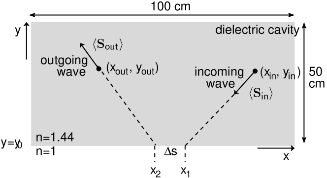
Figure 1: Extraction of the GHS $\Delta s$ from the measured incoming and outgoing beams. $\langle\mathbf{S}_{\text{in}}\rangle$ and $\langle\mathbf{S}_{\text{out}}\rangle$ are averaged Poynting vectors of the incoming and outgoing beams and $(x_{\text{in}},y_{\text{in}})$ and $(x_{\text{out}},y_{\text{out}})$ position averages. $x_{1}$ and $x_{2}$ are intersections of the straight lines defined by the Poynting vectors and averaged positions with $y=y_{0}$.

3 Beam generation

Microwave antennas produce spherical waves; for the GHS measurements, beams approximating plane waves have to be generated from these spherical waves. The generation of plane waves can be easily done because the superposition of $N$ spherical waves $\psi_{j}$ with wave number $k$ and centers $(x_{j},y_{j})$ on a straight line creates a beam

$$\psi(x,y)=\sum_{j=-N/2}^{j=N/2}\psi_{j}(x,y)=\sum_{j=-N/2}^{j=N/2}\frac{\exp\left[ik\sqrt{(x-x_{j})^{2}+(y-y_{j})^{2}}\right]}{\sqrt{(x-x_{j})^{2}+(y-y_{j})^{2}}}$$ (4)

which approaches a plane wave if $N$ goes to infinity. A similar generation of a suitable beam from multiple spherical waves generated by microwave antennas has been used in [20].

The propagation direction of a plane wave generated from spherical waves can be influenced by adding a phase factor $\phi(j)$ to each spherical wave. In this case, the generated beam is given by

$$\psi(x,y)=\sum_{j=-N/2}^{j=N/2}\psi_{j}(x,y)e^{i\phi(j)}$$ (5)

By varying $\phi(j)$, one can achieve propagation directions which lead to reflection under different angles of incidence. I.e., $\phi(j)=j$ leads to reflection with an angle below the critical angle $\chi_{\text{cr}}\approx 44$ degrees for Teflon with $n=1.44$, $\phi(j)=-j$ leads to reflection with an angle above the critical angle, and for $\phi(j)=0$ the reflection happens close to the critical angle. Unfortunately, there is no analytical formula for the relation of $\phi(j)$ and the resulting propagation direction; the choice of the $\phi(j)$ functions therefore remains somewhat arbitrary.

A plane wave, however, does not experience the GHS upon reflection, as the GH effect is a consequence of the interference of partial waves with different angles of incidence. Creating a plane wave thus does not suffice if one wants to measure the GHS. But by superposing two plane waves generated according to (5) with different $\phi(j)$ functions corresponding to a small difference in their propagation directions leads to a beam just like the one assumed in the derivation of the Artmann result:

$$\psi(x,y)=\psi_{1}(x,y)+\psi_{2}(x,y)\approx\exp\left(ikp_{1}x\right)+\exp\left(ikp_{2}x\right),$$ (6)

with $p_{m}=\sin\chi_{m}\sim S_{m,x}$, where $S_{m,x}$ is the $x$ component of the Poynting vector of partial wave $m$ (with $m=1,\,2$).

As both partial waves of the beam (6) are calculated using the same spherical wave components $\psi_{j}$,

$$\psi_{1}=\sum_{j=-N/2}^{N/2}\psi_{j}e^{i\phi_{1}(j)},\,\psi_{2}=\sum_{j=-N/2}^{N/2}\psi_{j}e^{i\phi_{2}(j)},$$ (7)

the sum is just given by

$$\psi=\psi_{1}+\psi_{2}=\sum_{j=-N/2}^{N/2}\psi_{j}\left(e^{i\phi_{1}(j)}+e^{i\phi_{2}(j)}\right).$$ (8)

In the experiment, measurements from $N=18$ antennas with positions $x_{j}=x_{A}+jd/\sqrt{2}$, $y_{j}=y_{A}-jd/\sqrt{2}$ with $x_{A}=40$ cm, $y_{A}=5$ cm and $d=0.5$ cm are superposed; the center of the coordinate system is the center of the Teflon plate (see figure 2). Because of the high resolution needed, it is not practical to measure the electric field on the whole Teflon plate, as it would take several years for the 18-antenna array. Instead, they are only measured on parts of it as indicated in figure 2. One such part lies on the incoming beam and one on the outgoing beam; the averages in (1) are performed over these fields. The third measured part is directly on the boundary of the Teflon plate. While it is not necessary for the extraction of the GHS, the data measured here allow the direct observation of the reflection process. Figure 2 shows the measured real parts $\text{Re}(\psi)$ of the beams generated according to (5) with $\phi_{j}=0$ at a frequency of $\nu=15$ GHz (corresponding to a vacuum wavelength $\lambda\approx 2$ cm). The boundary of the Teflon plate is shown, as well as the position of the $j=0$ antenna in the middle of the antenna array. It is clear from figure 2 that both the incoming and the outgoing beams have nearly plane wave fronts and travel at an angle of approximately 45 degrees to the plate boundary.

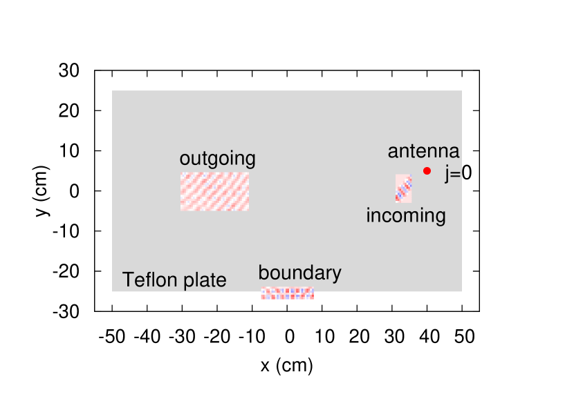
Figure 2: Measured real parts $\text{Re}(\psi)$ of the beams at $\nu=15$ GHz. The plate is indicated as the gray region; the position $(x_{A},y_{A})$ of the middle ($j=0$) antenna in the antenna array is shown as well.

4 Results

4.1 Generated “plane wave” beams

Details of the beams in the different measured parts of the Teflon plate are shown individually in figure 3 together with their Poynting vectors.

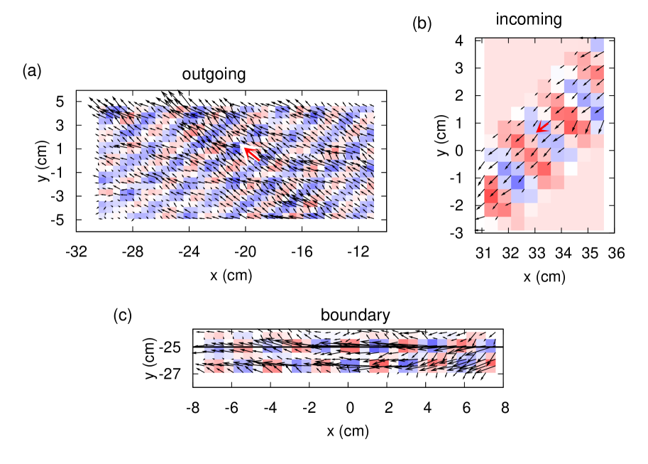
Figure 3: Real parts $\text{Re}(\psi)$ of the beams (color scale) and Poynting vectors (black arrows) in the three measured parts of the Teflon plate as shown in figure 2. (a) outgoing beam, (b) incoming beam, (c) beam at the plate boundary. The average Poynting vectors of the incoming and outgoing beams are shown as red arrows.

The positions $\mathbf{r}_{\text{in}}$ and $\mathbf{r}_{\text{out}}$ given by

$$\mathbf{r}_{\text{in}}=\pmatrix{33.5\cr 1.0}\text{ cm},\,\,\mathbf{r}_{\text{out}}=\pmatrix{-19.0\cr 0.0}\text{ cm}$$ (9)

for the Poynting vectors in this figure.

The spatial resolution of 5 mm is clearly sufficient to see the structure of the incoming and outgoing beams, which in fact approximate plane waves. Their respective Poynting vectors show a well-defined propagation direction. The incoming angle calculated from the averaged Poynting vector is $\chi\approx 47$ degrees, the respective outgoing angle is $\chi\approx 45$ degrees, which further supports the claim that, in fact, a plane wave travelling at an angle of 45 degrees has been created. The Poynting vectors of the beam at the boundary reveal – perhaps surprisingly given that so little can be seen in $\text{Re}\psi$ itself – that there are incoming and outgoing parts of the wave at the boundary. A part of it is reflected at the boundary, but another part penetrates outside the Teflon plate. The penetration depth seems to be a bit larger than the wavelength of 2 cm.

The generation of plane waves with one propagation direction thus works, at least for high $\nu$ values ($\nu\geq 10$ GHz; below that value, the wave fronts are less well defined and the extraction of Poynting vectors is thus not possible with high accuracy).

4.2 Extracted GHS

Two plane waves generated according to the scheme discussed in the previous section can now be superposed. The GHS of the resulting beam can be extracted and compared to the Artmann result. Table 1 shows the different phase functions $\phi_{1}(j),\,\phi_{2}(j)$ used in this section and the angle of incidence $\chi$ of the beam according to (8). The choice of the $\phi(j)$ functions is of course somewhat arbitrary; here, they are chosen such that the $j$ dependence is simple, the difference between $\phi_{1}(j)$ and $\phi_{2}(j)$ is small (as this is the approximation in the Artmann result), and such that a sufficiently broad range of angles of incidence results.

Table 1: Phase functions $\phi_{1,2}(j)$ and the resulting incoming angles $\chi$ in degrees as extracted from the experimental data.

• $\phi_{1}(j)$	$8j/9$	$2j/3$	$j/2$	$0$	$j/10$	$0$	$-j/2$	$-8j/9$
  $\phi_{2}(j)$	$j$	$3j/4$	$j/3$	$j/4$	$0$	$-j/4$	$-j/3$	$-j$
  $\chi$ (degrees)	22.5	27.9	35.1	41.4	44.9	47.6	55.9	68.9

The extracted GHS for the incoming angles given in table 1 is shown in figure 4 for $\nu=10$ GHz ($\lambda\approx 3$ cm) and $\nu=15$ GHz ($\lambda\approx 2$ cm) together with the Artmann result (10), which for TM polarization is given by

$$\Delta s=\frac{1}{nk\,\sin\chi}\frac{1}{\sqrt{\sin^{2}\chi-1/n^{2}}},$$ (10)

where $k=2\pi/\lambda$ is the wave number. $k\Delta s$ is thus independent of the wavelength.

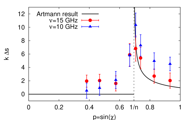
Figure 4: GHS $k\Delta s$ as extracted from the measured data for $\nu=15$ GHz (red dots) and $\nu=10$ GHz (blue triangles). The black solid line is the Artmann result, the black dashed line marks the critical angle for total internal reflection for $n=1.44$.

The error bars are the errors in $\langle\mathbf{S}\rangle_{\text{in (out)}}$, which in turn, as $\langle\mathbf{S}\rangle_{\text{in (out)}}$ is an average value, are given by the standard deviation. The error $\delta\Delta s$ in $\Delta s$ is then given by error propagation; the errors are all approximately $\delta\Delta s/\Delta s\approx 20$ % (incoming angles above the critical angle) and $\delta\Delta s/\Delta s\approx 50$ % (incoming angles below critical angle). As the GHS below the critical angle is small, larger relative errors are expected.

We see clear signatures of the GHS and the main features of the Artmann result (zero GHS below the critical angle, maximum GHS at the critical angle, approximately constant GHS above the critical angle, independence of $k\Delta s$ of $k$) are well captured. At $\nu=10$ GHz, the GHS is systematically higher than the Artmann result predicts. This is not surprising, as deviations due to the finite width of our generated beams can be expected to become larger for smaller frequencies.

In fact, the agreement of the measured GHS with theoretical predictions gets even better if the finite width of the beams is taken into account. The individual beams are not completely plane waves, as they have a width fixed by the width of the antenna array. If one approximates them as Gaussian (which is justified as Lai et al. [2] have shown that the precise beam profile has little influence on the resulting GHS) with a beam width given by the experimentally extracted value $\sigma\approx 3$ cm, the resulting GHS $\Delta s$ can be calculated numerically as described in [13]. Figure 5 shows the results together with the experimental data for $\nu=10$ GHz and $\nu=15$ GHz. The deviations above the critical angle are indeed explained very well by a Gaussian (non-plane wave) beam profile.

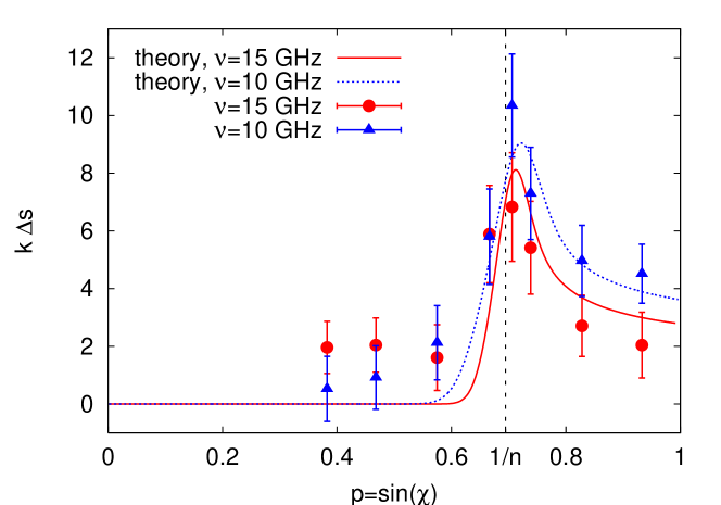
Figure 5: GHS $k\Delta s$ extracted from the measured data at $\nu=15$ GHz (red dots) and $\nu=10$ GHz (blue triangles). For comparison, the calculated GHS for a Gaussian wave packet with the corresponding frequency is shown as well (red solid and blue dotted curves). The black dashed line marks the critical angle for total internal reflection for $n=1.44$.

Overall, we find convincing agreement between the GHS extracted from our experimental data and the theoretical prediction of the Artmann result. The deviations of beams with smaller frequencies from the Artmann result are due to the finite width of our generated beams, as a numerical calculation of the GHS using a Gaussian beam profile with a beam width corresponding to the one found in our experiments shows.

5 Conclusions and outlook

We presented measurements of the Goos-Hänchen shift of microwave beams at a dielectric interface (Teflon to air). The beams were generated by superposing the spherical waves produced by 18 microwave antennas, which leads to beams with approximately plane wave fronts. The GHS is extracted from the Poynting vectors of the incoming and reflected beams, which can be found from measurements of the electric field of the beams. Our results agree well with the classical result of Artmann.

Our experiment demonstrates that GHS measurements in dielectric microwave cavities are possible and meaningful. A similar setup using not a rectangular Teflon plate, but one with curved boundaries, could be used to study the effects of boundary curvature on the GHS. When the GHS is incorporated into ray models, it is usually assumed that the curvature effects are small, and the GHS as calculated at a planar interface can be used. Microwave measurements could give insight into the question if and when this is possible, and what deviations can be expected. Another interesting experiment would be to excite modes in a microwave cavity and, by measuring electric fields, directly observe effects of the GHS which have been predicted in optical microcavities, e.g. the formation of new modes in an elliptical cavity [11] or the phase-space shift of periodic orbits [13].

References

References

- [1] Goos F and Hänchen H. Ein neuer und fundamentaler Versuch zur Totalreflexion. Ann. Phys., 1:333, 1947.
- [2] Lai H M, Cheng F C, and Tang W K. Goos-Hänchen effect around and off the critical angle. J. Opt. Soc. Am. A, 3:550, 1986.
- [3] de Haan V O, Plomp J, Rekveldt T M, Kraan W H, van Well A A, Dalgliesh R M, and Landridge S. Observation of Goos-Hänchen Shift with Neutrons. Phys. Rev. Lett., 104:010401, 2010.
- [4] Beenakker C W J, Sepkhanov R A, Akhmerov A R, and Tworzydło J. Quantum Goos-Hänchen Effect in Graphene. Phys. Rev. Lett., 102:146804, 2009.
- [5] Artmann K. Berechnung der Seitenversetzung des totalreflektierten Strahles. Ann. Phys., 2:87, 1948.
- [6] Artmann K. Brechung und Reflexion einer seitlich begrenzten (Licht-) Welle an der ebenen Trennfläche zweier Medien in Nähe des Grenzwinkels der Totalreflexion. Ann. Phys., 8:270, 1951.
- [7] Aiello A and Woerdman J P. Role of beam propagation in Goos-Hänchen and Imbert-Fedorov shifts. Opt. Lett., 33:1437, 2008.
- [8] Schwefel H G L, Köhler W, Lu Z H, Fan J, and Wang L J. Direct experimental observation of the single reflection optical Goos-Hänchen shift. Opt. Lett., 33:794, 2008.
- [9] Hentschel M and Schomerus H. Fresnel laws at curved dielectric interfaces of microresonators. Phys. Rev. E, 65:045603(R), 2002.
- [10] Schomerus H and Hentschel M. Correcting Ray Optics at Curved Dielectric Microresonator Interfaces: Phase-Space Unification of Fresnel Filtering and the Goos-Hänchen Shift. Phys. Rev. Lett., 96:243903, 2006.
- [11] Unterhinninghofen J, Wiersig J, and Hentschel M. Goos-Hänchen shift and localization of optical modes in deformed microcavities. Phys. Rev. E, 78:016201, 2008.
- [12] Altmann E G, del Magno G, and Hentschel M. Non-hamiltonian dynamics in optical microcavities resulting from wave-inspired corrections to geometric optics. Eur. Phys. Lett., 84:10008, 2008.
- [13] Unterhinninghofen J and Wiersig J. Interplay of Goos-Hänchen shift and boundary curvature in deformed microdisks. Phys. Rev. E, 82:026202, 2010.
- [14] Nöckel J U and Stone A D. Ray and wave chaos in asymmetric resonant optical cavities. Nature, 385:45, 1997.
- [15] Stöckmann H J. Quantum chaos: an introduction. Cambridge University Press, 2000.
- [16] Stein J and Stöckmann H J. Experimental Determination of Billiard Wave Functions. Phys. Rev. Lett., 68:2867, 1992.
- [17] Stein J, Stöckmann H J, and Stoffregen U. Microwave Studies of Billiard Green Functions and Propagators. Phys. Rev. Lett., 75:53, 1995.
- [18] Kuhl U. Wave functions, nodal domains, flow, and vortices in open microwave systems. Eur. Phys. J. Special Topics, 145:103, 2007.
- [19] Song Q, Cao H, Ho S T, and Solomon G S. Near-IR subwavelength microdisk lasers. Appl. Phys. Lett., 94:061109, 2009.
- [20] Oria Iriarte P. Double-slit experiments and decay probability in microwave billiards. PhD thesis, Technische Universität Darmstadt, 2010.