Partial Weyl Law for Billiards

Abstract

For two-dimensional quantum billiards we derive the partial Weyl law, i.e. the average density of states, for a subset of eigenstates concentrating on an invariant region $\Gamma$ of phase space. The leading term is proportional to the area of the billiard times the phase-space fraction of $\Gamma$. The boundary term is proportional to the fraction of the boundary where parallel trajectories belong to $\Gamma$. Our result is numerically confirmed for the mushroom billiard and the generic cosine billiard, where we count the number of chaotic and regular states, and for the elliptical billiard, where we consider rotating and oscillating states.

Waves restricted to finite resonators in two or three dimensions have found abundant applications in contemporary physics. Examples include electromagnetic and acoustic resonators, microdisk lasers, atomic matter waves in optical billiards, and quantum dots Sto1999 ; NoeSto1997 ; FriKapCarDav2001 ; ArcBaeCuaPriMenHer1998 ; MarRimWesHopGos1992 . The average density of states is an essential observable of a resonator and dictates many physical properties. Investigations of this quantity go back to Lord Rayleigh more than a hundred years ago Ray1877 and have been a continuing topic of interest ever since Wey1911 ; Wey1913 ; Kac1966 ; BalBloComb ; BalHil1976 ; BerHow1994 ; SiePriSmiUssSch1995 ; AreNitPetSte2009 . Today the fundamental result for the average density of states

$$\bar{d}(E)=\frac{A}{4\pi}-\frac{L}{8\pi}\frac{1}{\sqrt{E}}+\dots$$ (1)

is known as Weyl’s law, as he gave the first proof of the leading term Wey1911 . Equation (1) is formulated for the case of a two-dimensional quantum billiard with area $A$, boundary length $L$, and Dirichlet boundary conditions (in units $\hbar=2m=1$). Analogous results for three dimensions, other types of waves and boundary conditions are available AreNitPetSte2009 , and for open systems a fractal Weyl law was proposed LuSriZwo2003 .

The first term of eq. (1) depends on the area $A$ of the billiard only. As for any quantum system it is obtained by counting the number of Planck cells in the phase space available at energy $E$. The second term was already conjectured by Weyl Wey1913 . It is specific for billiards or resonators and depends on the length $L$ of the boundary. As the wave function must vanish on the boundary, a layer is depleted which has a length $L$ and a width of the order of the wave length $\lambda\sim 1/\sqrt{E}$. Semiclassically, the second term can be interpreted as a contribution from closed trajectories which are reflected perpendicularly at the boundary BalBloComb ; SieSmiCreLit1993 ; Hes1994 . Higher order corrections in eq. (1) arise, e.g., due to corners and curvature effects Kac1966 ; BalBloComb ; BalHil1976 ; BerHow1994 ; SiePriSmiUssSch1995 ; AreNitPetSte2009 .

Generic billiards, which are studied for electromagnetic, acoustic, and matter waves Sto1999 ; NoeSto1997 ; FriKapCarDav2001 ; ArcBaeCuaPriMenHer1998 , have a phase space containing several dynamically separated domains, such as regular and chaotic regions, see fig. 1(c). The spectrum consists of sub-spectra with eigenfunctions mainly concentrating on one of these invariant regions $\Gamma_{i}$, according to the semiclassical eigenfunction hypothesis Per1973 ; Ber1977 ; Vor1979 . It is a fundamental question to know the corresponding partial average density of states $\bar{d}_{\Gamma_{i}}(E)$, where $\bar{d}(E)=\sum_{i}\bar{d}_{\Gamma_{i}}(E)$. This is essential for studying the spectral statistics Haa2000 of such sub-spectra. The partial density of states is also compulsory for the determination of transition rates with Fermi’s golden rule BaeKetLoeRobVidHoeKuhSto2008 . Furthermore, it is required when an external coupling to the system is not uniform in phase space, e.g., the total internal reflection in optical resonators HacVivElaHaa2001 ; Sto2001 or tilted leads attached to a quantum dot BirAkiFerVasCooAoySug1999 .

In this paper we derive the partial Weyl law,

$$\bar{d}_{\Gamma}(E)=\frac{A_{\Gamma}}{4\pi}-\frac{L_{\Gamma}}{8\pi}\frac{1}{\sqrt{E}},$$ (2)

for a subset of eigenstates corresponding to an invariant region $\Gamma$ of phase space, using the Wigner-Weyl transformation of the Green function. As expected, for the area $A_{\Gamma}$ the ratio $A_{\Gamma}/A$ is the fraction of phase space occupied by $\Gamma$, see eq. (14). For the length $L_{\Gamma}$ we find that the ratio $L_{\Gamma}/L$ is the fraction of the billiard boundary where parallel trajectories belong to $\Gamma$, see eq. (15). This is unexpected as semiclassically the boundary term in eq. (1) originates from trajectories perpendicular to the boundary BalBloComb ; SieSmiCreLit1993 ; Hes1994 . We confirm the result eq. (2) numerically for the mushroom billiard and the generic cosine billiard, where we predict the number of regular and chaotic states, and for the elliptical billiard, where we consider rotating and oscillating states.

Before we derive eq. (2) we exemplify its application for the desymmetrized mushroom billiard Bun2001 shown in fig. 1(c). It is characterized by the radius $R$ of the quarter circular cap, the stem width $a$, and the stem height $l$. Classically one has two distinct phase-space regions visualized in fig. 1(c). All trajectories which are located only in the cap of the mushroom are regular, while those entering the stem are chaotic Bun2001 . For the chaotic region eq. (14) yields $A_{\text{ch}}=\pi R^{2}/4-[R^{2}\arcsin(a/R)+a\sqrt{R^{2}-a^{2}}]/2$ BaeKetLoeRobVidHoeKuhSto2008 . For the length $L_{\text{ch}}$ we have to consider those parts of the billiard boundary $\partial\Omega$ for which parallel trajectories belong to the chaotic region (including the marginally stable bouncing-ball orbits). This is the case for the straight boundaries, such that $L_{\text{ch}}=2R+2l$ is the length of the chaotic boundary of the mushroom billiard. $A_{\text{reg}}$ and $L_{\text{reg}}$ follow from $A_{\text{reg}}=A-A_{\text{ch}}$ and $L_{\text{reg}}=L-L_{\text{ch}}=\pi R/2$, respectively. (For the full mushroom billiard one finds $L_{\text{reg}}=\pi R$ and $L_{\text{ch}}=2R+2l$.) In order to verify this prediction of the partial density of states, eq. (2), we numerically solve the time-independent Schrödinger equation, $-\Delta\psi_{l}({\bf q})=E_{l}\psi_{l}({\bf q})$, for the desymmetrized mushroom billiard with Dirichlet boundary condition ($\psi_{l}({\bf q})=0$, ${\bf q}\in\partial\Omega$), $R=1$, $l=1$, and $a=0.5$. We calculate the first $6024$ eigenstates $\psi_{l}$ using the improved method of particular solutions BetTre2005 . They can be classified as mainly regular or mainly chaotic, depending on the phase-space region on which they concentrate (fig. 1(c)). There are several methods for this classification which give similar results. Here we determine the regular fraction $w_{\text{reg}}^{l}$ of an eigenstate $\psi_{l}$ of the mushroom by its projection on a basis of the regular region. For this basis we use the eigenstates $\psi_{\text{qc}}^{mn}$ of a quarter circle of radius $R=1$ with energy $E_{mn}$ and angular momentum $m>a\sqrt{E_{mn}}$. These basis states are given by $\psi_{\text{qc}}^{mn}(r,\varphi)=N_{mn}J_{m}(j_{mn}r)\sin(m\varphi)$, where $m=2,4,\dots$ is the angular quantum number, $n=1,2,\dots$ is the radial quantum number, $J_{m}$ is the $m$th Bessel function of the first kind, $j_{mn}$ is the $n$th root of $J_{m}$, $E_{mn}=j_{mn}^{2}$, and $N_{mn}=\sqrt{8/\pi}/J_{m-1}(j_{mn})$ is a normalization constant. The projection of $\psi_{l}$ onto these basis states leads to the regular fraction $w_{\text{reg}}^{l}=\sum_{m,n}|\langle\psi_{\text{qc}}^{mn}|\psi_{l}\rangle|^{2}\,\Theta(m-a\sqrt{E_{mn}})$ with $0\leq w_{\text{reg}}^{l}\leq 1$. The chaotic fraction is then given by $w_{\text{ch}}^{l}=1-w_{\text{reg}}^{l}$. From $w_{\text{reg}}^{l}$ and $w_{\text{ch}}^{l}$ the densities of the regular and the chaotic states can be computed, $d_{\Gamma}(E)=\sum_{l}w_{\Gamma}^{l}\,\delta(E-E_{l})$. For comparison with numerics we use the more convenient spectral staircase function $N_{\Gamma}(E)=\int_{0}^{E}\text{d}\eta\,d_{\Gamma}(\eta)$. It has a step of size $w_{\Gamma}^{l}$ at eigenenergy $E_{l}$. From eq. (2) one finds

$$\bar{N}_{\Gamma}(E)=\frac{A_{\Gamma}}{4\pi}E-\frac{L_{\Gamma}}{4\pi}\sqrt{E}.$$ (3)

Figure 1(a) shows the regular and the chaotic spectral staircase for the mushroom billiard. We find excellent agreement with our prediction, eq. (3) (smooth solid lines). In fig. 1(b) we demonstrate that the boundary contribution of eq. (3) is in agreement with the difference of the numerical data and the first term of eq. (3). Using the semiclassical interpretation of the boundary term in eq. (1) one would naively expect that $L_{\Gamma}/L$ is the fraction of the boundary where perpendicular trajectories belong to $\Gamma$. However, this does not reproduce the data (dotted lines). The numerical fluctuations arise due to oscillatory contributions to the density of states which are not considered here. We have confirmed that under variation of the width $a$ of the stem of the mushroom the prediction eq. (3) agrees with numerics.

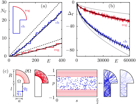
Figure 1: (Color online) (a) Spectral staircase $N_{\Gamma}(E)$ for regular and chaotic eigenstates of the desymmetrized mushroom billiard with $R=1$, $l=1$, and $a=0.5$. We compare numerical data with the first term (dashed lines) and both terms of eq. (3) (smooth solid lines). The inset shows the regular and chaotic parts of the boundary. (b) Same data after subtracting the area term, $\Delta_{\Gamma}(E)=N_{\Gamma}(E)-A_{\Gamma}E/(4\pi)$, compared to the second term of eq. (3) (smooth solid lines) shown over a larger energy range. Determining $L_{\Gamma}$ in eq. (3) from perpendicular instead of parallel trajectories gives an incorrect result (dotted lines). (c) Phase space at the circular boundary with regular (lines) and chaotic (dots) regions and illustrations of trajectories and eigenfunctions.

Now we turn to the derivation of eq. (2). The most general method to represent quantum states in phase space is their Wigner distribution. Other options, such as the Husimi distribution or numerical methods for specific geometries as in the example above, yield similar results and can be obtained from averages over the Wigner distribution. In the semiclassical limit, according to the semiclassical eigenfunction hypothesis, the weights $w^{l}_{\Gamma}$ for an invariant region $\Gamma$ of non-zero measure are either zero or one and independent of the projection method.

Based on the Wigner distribution of an eigenstate $\psi_{l}$,

$$W_{l}({\bf q},{\bf p})=\frac{1}{\pi^{2}}\int\text{d}^{2}{\bf r}\,\text{e}^{2\text{i}{\bf p}{\bf r}}\psi_{l}^{*}({\bf q}+{\bf r})\psi_{l}({\bf q}-{\bf r}),$$ (4)

we define the phase-space resolved density of states for a phase-space point $({\bf q},{\bf p})$

$$d_{{\bf q},{\bf p}}(E)=\sum_{l=1}^{\infty}\delta(E-E_{l})\,W_{l}({\bf q},{\bf p}).$$ (5)

For an arbitrary region $\Gamma$ of phase space the density of states is given by the integral

$$d_{\Gamma}(E)=\int_{\Gamma}\text{d}^{2}{\bf q}\,\text{d}^{2}{\bf p}\,d_{{\bf q},{\bf p}}(E).$$ (6)

Using

$$\text{Im}\,G({\bf x},{\bf x}^{\prime},E)=-\pi\sum_{l=1}^{\infty}\psi_{l}^{*}({\bf x}^{\prime})\psi_{l}({\bf x})\delta(E-E_{l})$$ (7)

eq. (5) can be rewritten as

$$d_{{\bf q},{\bf p}}(E)=-\frac{1}{\pi^{3}}\int\text{d}^{2}{\bf r}\,\text{e}^{2\text{i}{\bf p}{\bf r}}\,\text{Im}\,G({\bf q}-{\bf r},{\bf q}+{\bf r},E),$$ (8)

where $G({\bf x},{\bf x}^{\prime},E)$ is the energy dependent Green function. For billiards it satisfies

$$(\Delta+\kappa^{2})G({\bf x},{\bf x}^{\prime},E)=\delta({\bf x}-{\bf x}^{\prime}),\quad{\bf x},{\bf x}^{\prime}\in\Omega,$$ (9)

where $\kappa=\sqrt{E}$. On $\partial\Omega$ it satisfies the boundary condition of the billiard and is zero outside $\Omega$. Close to the boundary the curvature can be neglected and the Green function of a half-plane is an appropriate approximation. It is then given in the upper half-plane by

$$G({\bf x},{\bf x}^{\prime},E)\approx\frac{1}{4\text{i}}[H_{0}^{+}(\kappa|{\bf x}-{\bf x}^{\prime}|)-H_{0}^{+}(\kappa|{\bf x}-\hat{\bf x}^{\prime}|)].$$ (10)

Here $H_{0}^{+}$ denotes the Hankel function of the first kind and $\hat{\bf x}^{\prime}$ is the mirror image of ${\bf x}^{\prime}$.

Instead of requiring that the Green function vanishes in the lower half-plane, it is more appropriate to continue the Green function antisymmetrically across the boundary, i.e. eq. (10) is extended to the full plane. In this way the corresponding Wigner function is adapted to the Dirichlet boundary condition and yields a more faithful momentum distribution FOOTNOTE . Far from the boundary this modification has no effect and reduces to the standard definition.

Using polar coordinates for the momentum ${\bf p}=(p,\beta)$ and Cartesian coordinates for the position ${\bf q}=(q_{\parallel},q_{\perp})$, measured parallel and perpendicular to the boundary $\partial\Omega$, we evaluate in eq. (8) the integrals over ${\bf r}$ and in eq. (6) the integral over $p$,

$$\bar{d}_{{\bf q},\beta}(E) = \frac{1}{4\pi^{3}}\int_{0}^{\infty}\text{d}p\,p\int\text{d}^{2}{\bf r}\,\text{e}^{2\text{i}{\bf p}{\bf r}}$$ (11)

$$\times\left[J_{0}(2\kappa|r|)-J_{0}\left(2\kappa\sqrt{r_{\parallel}^{2}+q_{\perp}^{2}}\right)\right],$$

where $J_{0}$ is the Bessel function of the first kind. For the ${\bf r}$-integration of the first Bessel function we use polar coordinates ${\bf r}=(r,\varphi)$, where $\varphi$ is the angle with respect to ${\bf p}$, $\oint\text{d}\varphi\,\text{e}^{2\text{i}pr\cos\varphi}=2\pi J_{0}(2pr)$, and $\int_{0}^{\infty}\text{d}r\,r\,J_{0}(2pr)J_{0}(2\kappa r)=\delta(p-\kappa)/4p$. For the ${\bf r}$-integration of the second Bessel function in eq. (11) we use Cartesian coordinates ${\bf r}=(r_{\parallel},r_{\perp})$ leading to ${\bf p}{\bf r}=pr_{\parallel}\cos(\beta-\beta_{\parallel})+pr_{\perp}\sin(\beta-\beta_{\parallel})$, where $\beta_{\parallel}({\bf q})$ is the angle of the tangent to the boundary at ${\bf q}\in\partial\Omega$. Integration over $r_{\perp}$ gives $\pi\delta(\sin[\beta-\beta_{\parallel}])/p$ and integration over $p$ leads to $\pi\delta(r_{\parallel})/2$. Finally we obtain

$$\bar{d}_{{\bf q},\beta}(E)=\frac{1}{8\pi^{2}}-\frac{1}{8\pi}\delta(\sin[\beta-\beta_{\parallel}])J_{0}(2\kappa q_{\perp}).$$ (12)

The $\delta$-function selects trajectories with momentum parallel to the boundary. According to eq. (6) we have

$$\bar{d}_{\Gamma}(E)=\int_{\Omega}\text{d}^{2}{\bf q}\int_{0}^{2\pi}\text{d}\beta\,\chi_{\Gamma}({\bf q},\beta)\,\bar{d}_{{\bf q},\beta}(E),$$ (13)

where $\chi_{\Gamma}({\bf q},\beta)$ is the characteristic function of the phase-space region $\Gamma$. It is one when the trajectory running at angle $\beta$ through the point ${\bf q}$ belongs to $\Gamma$, zero if this is not the case, and $1/2$ on the boundary of $\Gamma$. We now evaluate eq. (13) in the semiclassical limit $\kappa\to\infty$, where $J_{0}(2\kappa q_{\perp})\to\delta(q_{\perp})/\kappa$. This gives the final result eq. (2) with

$$A_{\Gamma} = \int_{\Omega}\text{d}^{2}{\bf q}\,\frac{1}{2\pi}\int_{0}^{2\pi}\text{d}\beta\,\chi_{\Gamma}({\bf q},\beta),$$ (14)

$$L_{\Gamma} = \oint_{\partial\Omega}\text{d}s\,\chi_{\Gamma}({\bf q}(s),\beta_{\parallel}(s)).$$ (15)

Here, $s$ is the arc length along the boundary, ${\bf q}(s)$ is the corresponding point on the boundary, and $\beta_{\parallel}(s)=\beta_{\parallel}({\bf q}(s))$ is the angle of the tangent to the boundary at that point. We thus find that $L_{\Gamma}/L$ is the fraction of the billiard boundary where parallel trajectories belong to $\Gamma$. Strictly speaking, $\chi_{\Gamma}({\bf q}(s),\beta_{\parallel}(s))$ in eq. (15) is obtained as a limit from trajectories starting at $q_{\parallel}=s$ with $\beta\to\beta_{\parallel}$ and $q_{\perp}\to 0$. This infinitesimal neighborhood has to be considered when the parallel trajectory with $\beta=\beta_{\parallel}$ and $q_{\perp}=0$ cannot be assigned to one of the regions $\Gamma$. Note, that $A_{\Gamma}$ is proportional to the volume of $\Gamma$, while there is no such simple relation for $L_{\Gamma}$. For the special case where $\Gamma$ is the entire phase space we have $\chi_{\Gamma}\equiv 1$ leading to $A_{\Gamma}=A$ and $L_{\Gamma}=L$, such that eq. (2) reduces to eq. (1).

We now give two explanations for the boundary term in eq. (2) and its relation to trajectories of $\Gamma$ that are parallel to the boundary: (i) If $\Gamma$ is the entire phase space eqs. (6) and (8) lead to $d_{{\bf q}}(E)=-\text{Im}\,G({\bf q},{\bf q},E)/\pi$. The semiclassical contributions to this Green function are given by closed trajectories which start and end at ${\bf q}$ Sto1999 . According to the second term in eq. (10) they have a length $2q_{\perp}$ corresponding to a perpendicular reflection at the boundary. This leads to the term $J_{0}(2\kappa q_{\perp})/(4\pi)$, which agrees with the second term in eq. (12) when integrated over all $\beta$. If $\Gamma$ is a region in phase space, one needs the phase-space resolved density of states $d_{{\bf q},{\bf p}}(E)$. Equation (8) shows that the direction of the momentum ${\bf p}$ is not related to the direction of the trajectories which semiclassically contribute to the Green function. Evaluating eq. (11) leads to $r_{\parallel}=0$, such that still perpendicularly reflected trajectories of length $2q_{\perp}$ give the boundary term. However, this contribution arises only if the direction $\beta$ of the momentum ${\bf p}$ is parallel to the boundary. For the other directions the contribution cancels due to the phase factor $\exp(2\text{i}{\bf p}{\bf r})$ in eq. (11). (ii) An intuitive explanation of the boundary term can be given in terms of a plane wave, $\exp(\text{i}p_{\parallel}q_{\parallel})\sin(p_{\perp}q_{\perp})$, with Dirichlet boundary condition at $q_{\perp}=0$. Here the sine-term suppresses waves with $p_{\perp}=0$ and thus reduces the density of states for these waves, which have a momentum ${\bf p}$ parallel to the boundary. Semiclassically such waves correspond to trajectories parallel to the boundary, in agreement with our result for the boundary term, eq. (15).

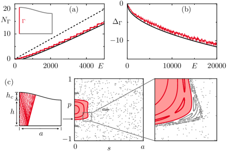
Figure 2: (Color online) (a) Spectral staircase $N_{\Gamma}(E)$ for eigenstates concentrated in an invariant region $\Gamma$ of the desymmetrized cosine billiard with $a=1.3$, $h=0.8$, and $h_{c}=0.24$. We compare numerical data with the first term (dashed line) and both terms of eq. (3) (smooth solid line). The inset shows the part of the boundary corresponding to $\Gamma$. (b) Same data after subtracting the area term, $\Delta_{\Gamma}(E)=N_{\Gamma}(E)-A_{\Gamma}E/(4\pi)$, compared to the second term of eq. (3) (smooth solid line) shown over a larger energy range. (c) Phase space at the lower horizontal boundary with invariant region $\Gamma$ (red shaded), remaining phase space (gray lines and dots), magnification of the hierarchical regular-to-chaotic transition region, and illustration of a regular trajectory.

We now consider the desymmetrized cosine billiard in order to demonstrate that the partial Weyl law can be applied to systems with a generic mixed phase-space structure. The cosine billiard is characterized by the height $h$ and length $a$ of the rectangular part as well as the height $h_{c}$ of the upper cosine boundary, see fig. 2(c). For the chosen parameters the phase-space of the cosine billiard consists of one large regular region surrounded by chaotic motion and a four-island resonance chain, see fig. 2(c), which also shows a magnification of the generic hierarchical regular-to-chaotic transition region. In order to apply the partial Weyl law we have to define a region $\Gamma$ in phase space and determine the corresponding area $A_{\Gamma}$ and length $L_{\Gamma}$. According to eq. (3) this gives a prediction for the number of eigenstates concentrating on $\Gamma$. In principle any invariant region can be used. We choose the red-shaded region in fig. 2(c), which contains most of the central regular island. The area $A_{\Gamma}$ is determined from eq. (14) by numerical integration. For the length $L_{\Gamma}$ we have to consider those parts of the billiard boundary $\partial\Omega$ for which parallel trajectories belong to $\Gamma$. This holds for the left vertical boundary of length $L_{\Gamma}=h+h_{c}$, see the inset in fig. 2(a). We stress, that including the hierarchical region or parts thereof in the definition of $\Gamma$ affects $A_{\Gamma}$, but not the boundary term $L_{\Gamma}$, as the orbits parallel to the boundary do not belong to the hierarchical transition region. Numerically we calculate the first $1853$ eigenstates of the desymmetrized cosine billiard with $h=0.8$, $a=1.3$, and $h_{c}=0.24$ using the improved method of particular solutions BetTre2005 . For the $l$th eigenstate we integrate its Poincaré-Husimi distribution BaeFueSch2004 over the region corresponding to $\Gamma$ which gives the weight $w_{\Gamma}^{l}$. These weights determine the spectral staircase function $N_{\Gamma}(E)$. We find excellent agreement with our prediction, eq. (3), see fig. 2(a). In fig. 2(b) we demonstrate that the boundary contribution of eq. (3) is in agreement with the difference of the numerical data and the first term of eq. (3), apart from a constant offset due to higher order terms neglected in eq. (3).

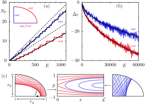
Figure 3: (Color online) (a) Spectral staircase $N_{\Gamma}(E)$ for rotating and oscillating eigenstates of the desymmetrized elliptical billiard with $r_{a}=1$ and $r_{b}=0.7$. We compare numerical data with the first term (dashed lines) and both terms of eq. (3) (smooth solid lines). The inset shows the rotating and oscillating parts of the boundary. (b) Same data after subtracting the area term, $\Delta_{\Gamma}(E)=N_{\Gamma}(E)-A_{\Gamma}E/(4\pi)$, compared to the second term of eq. (3) (smooth solid lines) shown over a larger energy range. (c) Phase space at the elliptical boundary with rotating (red lines from left to right) and oscillating (blue lines) regions and illustrations of trajectories.

As an interesting application, where a part of the boundary contributes to two invariant regions of phase space, we now consider the desymmetrized elliptical billiard WaaWieDull1997 , shown in fig. 3(c). It is characterized by the lengths $r_{a}$ and $r_{b}$ of the two half-axes, with $r_{a}>r_{b}$, and the focus $f=\sqrt{r_{a}^{2}-r_{b}^{2}}$. The phase space of the elliptical billiard consists of two separated regions of rotating and oscillating motion as visualized in fig. 3(c). The quantum eigenstates can be classified accordingly as mainly rotating or oscillating, $\bar{N}(E)=\bar{N}_{\text{rot}}(E)+\bar{N}_{\text{osc}}(E)$. Using eq. (3) we predict the number of rotating and oscillating states up to energy $E$. The areas $A_{\text{rot}}$ and $A_{\text{osc}}$ are determined from eq. (14) by numerical integration. For the length $L_{\text{rot}}$ we have to consider those parts of the billiard boundary $\partial\Omega$ for which parallel trajectories show rotating motion. This is the case for the elliptical boundary of length $\mathcal{L}$. Trajectories parallel to the horizontal boundary are precisely on the separatrix between oscillating and rotating motion. Therefore, integration over $\delta(\sin\beta)$ in eq. (12) gives half of the contribution for each of the two invariant regions of phase space and we have $L_{\text{rot}}=\mathcal{L}+r_{a}/2$. For the oscillating states we have $L_{\text{osc}}=r_{b}+r_{a}/2$. Note, that for the full ellipse the complete boundary belongs to the rotating region, $L_{\text{rot}}=4\mathcal{L}$ and $L_{\text{osc}}=0$. Numerically we calculate the first $2568$ eigenstates of the desymmetrized elliptical billiard with $r_{a}=1.0$ and $r_{b}=0.7$ using the improved method of particular solutions BetTre2005 . They are characterized by the angular and the radial quantum number $m$ and $n$. For each state we calculate the second constant of motion $\kappa_{mn}$ WaaWieDull1997 . If $\kappa_{mn}^{2}>f^{2}$ the state is classified as rotating and for $\kappa_{mn}^{2}<f^{2}$ as oscillating. Figure 3(a) shows the rotating and the oscillating spectral staircase for the elliptical billiard. We find excellent agreement with our prediction, eq. (3) (smooth solid lines). In fig. 3(b) we demonstrate that the boundary contribution of eq. (3) is in agreement with the difference of the numerical data and the first term of eq. (3). We have confirmed that also under variation of $r_{b}$ the prediction eq. (3) agrees with numerics (not shown).

A straightforward generalization of our results to Neumann boundary conditions is possible by changing the sign of the second term in eqs. (2), (3), (10), and (12). As interesting tasks there remains to find the higher order terms of $\bar{d}_{\Gamma}(E)$ due to corners and curvature effects as well as to generalize our approach to systems with broken time-reversal symmetry and to three-dimensional cavities. Also the generalization of the approach to systems with smooth potentials BohTomUll1993 is an open problem. Finally, it is now possible to study the spectral fluctuations around $\bar{d}_{\Gamma}(E)$ associated with a phase-space region $\Gamma$ for generic billiards.

We thank M. Sieber for valuable discussions and the DFG for support within the Forschergruppe 760 ”Scattering Systems with Complex Dynamics”.

References

- (1) H.-J. Stöckmann, Quantum Chaos. An introduction (University Press, Cambridge, 1999).
- (2) J. U. Nöckel and A. D.Stone, Nature 385, 45 (1997).
- (3) N. Friedman, A. Kaplan, D. Carasso, and N. Davidson, Phys. Rev. Lett. 86, 1518 (2001).
- (4) E. Arcos, G. Baez, P. A. Cuatlayol, M. L. H. Prian, R. A. Mendez-Sanchez, and H. Hernandez-Saldana, Am. Jour. Phys. 66, 601 (1998).
- (5) C. M. Marcus, A. J. Rimberg, R. M. Westervelt, P. F. Hopkins, and A. C. Gossard, Phys. Rev. Lett. 69, 506 (1992).
- (6) J. W. S. Rayleigh, The Theory of Sound, Vol. 2 (Dover, 1877).
- (7) H. Weyl, Nach. Akad. Wiss. Göttingen, 110 (1911).
- (8) H. Weyl, J. Reine Angew. Math. 143, 177 (1913).
- (9) M. Kac, Am. Math. Monthly 73, 1 (1966).
- (10) R. Balian and C. Bloch, Ann. Phys. (N.Y.) 60, 401 (1970); 84, 559(E) (1974); 69, 76 (1972).
- (11) H. P. Baltes and E. R. Hilf, Spectra of Finite Systems (Bibliographisches Institut, Mannheim, 1976).
- (12) M. Berry and C. Howls, Proc. R. Soc. London, Ser. A 447, 527 (1994).
- (13) M. Sieber, H. Primack, U. Smilansky, I. Ussishkin, and H. Schanz, J. Phys. A 28, 5041 (1995).
- (14) W. Arendt, R. Nittka, W. Peter, and F. Steiner, in Mathematical Analysis of Evolution, Information, and Complexity., edited by W. Arendt and W. P. Schleich (WILEY-VCH, Weinheim, 2009).
- (15) W. T. Lu, S. Sridhar, and M. Zworski, Phys. Rev. Lett. 91, 154101 (2003).
- (16) M. Sieber, U. Smilansky, S. C. Creagh, and R. G. Littlejohn, J. Phys. A 26, 6217 (1993).
- (17) T. Hesse, Die spektrale Stufenfunktion des abgeschnittenen Hyperbelbillards, Diploma thesis, Hamburg (1994).
- (18) I. C. Percival, J. Phys. B 6, L229 (1973).
- (19) M. V. Berry, J. Phys. A 10, 2083 (1977).
- (20) A. Voros, in Stochastic Behavior in Classical and Quantum Hamiltonian Systems (Springer-Verlag, Berlin, 1979).
- (21) F. Haake, Quantum Signatures of Chaos (Springer-Verlag, Berlin, 2000).
- (22) A. Bäcker, R. Ketzmerick, S. Löck, M. Robnik, G. Vidmar, R. Höhmann, U. Kuhl, and H.-J. Stöckmann, Phys. Rev. Lett. 100, 174103 (2008).
- (23) G. Hackenbroich, C. Viviescas, B. Elattari, and F. Haake, Phys. Rev. Lett. 86, 5262 (2001).
- (24) D. Stone, Physica Scripta T90, 248 (2001).
- (25) J. P. Bird, R. Akis, D. K. Ferry, D. Vasileska, J. Cooper, Y. Aoyagi, and T. Sugano, Phys. Rev. Lett. 82, 4691 (1999).
- (26) L. A. Bunimovich, Chaos 11, 802 (2001).
- (27) T. Betcke and L. N. Trefethen, SIAM Rev. 47, 469 (2005).
- (28) The standard Wigner function maps a plane wave to a sharp peak in momentum. However, this clear correspondence is lost if the domain of the wave function is restricted in space, as it is the case in a billiard. For a point close to the boundary the integral in eq. (4) covers only a small spatial interval and results in a broad momentum distribution. The boundary adapted Wigner function avoids this artifact of the restricted domain BaeKetLoeSchFUTURE . For example, in 1D the transform of a sine wave has the expected -peaks at . Note, that the standard Wigner function would result in eq. (12) in a broad distribution of for points near the boundary.
- (29) A. Bäcker, R. Ketzmerick, S. Löck, and H. Schanz, in preparation.
- (30) A. Bäcker, S. Fürstenberger, and R. Schubert, Phys. Rev. E 70, 036204 (2004).
- (31) H. Waalkens, J. Wiersig, and H. R. Dullin, Ann. Phys. (N.Y.) 260, 50 (1997).
- (32) O. Bohigas, S. Tomsovic, and D. Ullmo, Phys. Rep. 223, 42 (1993).