Robust Tests in Genome-Wide Scans under Incomplete Linkage Disequilibrium

Abstract

Under complete linkage disequilibrium (LD), robust tests often have greater power than Pearson’s chi-square test and trend tests for the analysis of case-control genetic association studies. Robust statistics have been used in candidate-gene and genome-wide association studies (GWAS) when the genetic model is unknown. We consider here a more general incomplete LD model, and examine the impact of penetrances at the marker locus when the genetic models are defined at the disease locus. Robust statistics are then reviewed and their efficiency and robustness are compared through simulations in GWAS of 300,000 markers under the incomplete LD model. Applications of several robust tests to the Wellcome Trust Case-Control Consortium [Nature 447 (2007) 661–678] are presented.

, , , and

1 Introduction

Genome-wide association studies (GWAS) have been used to detect true associations between 100,000 to 500,000 genetic markers (single-nucleotide polymorphisms—SNPs) and common or complex diseases (e.g., Klein et al., 2005; Sladek et al., 2007; WTCCC, 2007). Currently, up to a million SNPs are used in GWAS. A simple and initial analysis of GWAS is a genome-wide scan, in which a statistical test is applied to detect association one SNP at a time. Test statistics and/or their $p$-values are obtained for all SNPs and ranked in order of their statistical significance. After all SNPs are ranked, a prespecified small proportion of SNPs from the top-ranked SNPs (or SNPs with $p$-values less than a prespecified genome-wide threshold level) is selected for further, more focused analyses, for example, haplotype analysis, multi-marker analysis, fine mapping, imputation and independent replication studies (see Hoh and Ott, 2003; Marchini, Donnelly and Cardon, 2005; Schaid et al., 2005). The genome-wide scan has also been shown to be cost-effective in two-stage designs for GWAS, in which additional subjects are genotyped in the second stage for a small portion of selected SNPs in the first stage (see Elston, Lin and Zheng, 2007; Thomas et al., 2009). We focus on robust tests for GWAS in the single stage designs.

Since only a small portion of top-ranked SNPs is selected in genome-wide scans, it is important that the probability of at least one SNP with true association being selected is high, for example, greater than 80% (Zaykin and Zhivotovsky, 2005; Gail et al., 2008). The probability that a SNP with true association is detected, confirmed and replicated in later more focused analyses is often smaller. Hence, one of the goals of genome-wide scans is to rank the SNPs with true associations as near to the top as possible. Zaykin and Zhivotovsky (2005) showed that the factors that mainly affect the rankings of true SNPs include the total number of SNPs, the number of SNPs with true associations, the genetic effects (genotype relative risks or odds ratios), the sample size, power of the association test used, and linkage disequilibrium (LD) between SNPs and the functional locus (the true unknown disease locus). Most of the above factors are determined by the study design, except the power of the test for association. The common association tests include Pearson’s chi-squared test (Pearson’s test, for short), the Cochran-Armitage trend tests (CATTs) and the allelic test. Three CATTs are available depending on the underlying genetic model (the mode of inheritance of the disease locus). Common genetic models include recessive, additive, multiplicative and dominant models. Overdominant and underdominant models may also be used, but they are less common. The allelic test has performance similar to that of the CATT under the additive model when the Hardy–Weinberg equilibrium proportions hold (Sasieni, 1997; Guedj, Nuel and Prum, 2008). Thus, the allelic test is not considered here.

Intuitively, the most powerful test should be used in genome-wide scans. For common and complex diseases, it is possible that there are multiple functional loci with different genetic models, in particular, for GWAS. The power of an association test depends on the underlying genetic models of the functional loci, which, however, are unknown. They could be any of the four common genetic models or none of them. In addition, imperfect LD between functional and marker loci can modify the underlying genetic model, further increasing uncertainty. In this case, there is no uniformly most powerful test for a genome-wide scan. It is known that the most efficient CATT is available when the genetic model is known (Sasieni, 1997; Freidlin et al., 2002). When the genetic model is unknown, using a single CATT is not robust across a family of genetics models. Therefore, in this situation, more robust tests have been proposed for both candidate-gene studies and genome-wide scans (Freidlin et al., 2002; Sladek et al., 2007; Zheng and Ng, 2008; Gonzalez et al., 2008; Joo et al., 2009). The performance of the robust test statistics has been studied under the perfect LD model, that is, the SNP is the same as the functional locus (see more discussion later). This is, however, a strong assumption for GWAS. In particular, when one of the models embedded into a robust test holds at the functional locus, it remains unmodified at the marker locus. Therefore, it is not surprising that robust tests based on the maximum of test statistics over common genetic models often provide greater power than Pearson’s test and CATTs. However, when LD is imperfect, the induced penetrance values at the marker are weighted averages of the causal penetrances, where the weights are functions of LD. Thus, the imperfect LD will change certain models, such as the dominant or the recessive models, so that the heterozygote penetrance will have an intermediate value between those for the homozygotes. Therefore, it is important to investigate not only the exact form of such penetrance modifications, but also its impact on the performance of the robust tests for association.

In this article we consider a general LD model with the standardized LD parameter, $D^{\prime}$ (Lewontin, 1964), and study the properties of the penetrances defined at the marker locus given the genetic model defined at the functional locus. In addition to reviewing some common robust tests for case-control association studies, we also compare their performance under this general model with a varying $D^{\prime}$. Using robust tests when there is imperfect LD has not been studied perviously. The perfect LD case, where the marker and the disease loci coincide, can be obtained as a special case at $D^{\prime}=1$, with an additional requirement of equality of allele frequencies at the marker and the disease locus. This implies a perfect correlation between the alleles at the two loci. Under this general model, we also examine the effectiveness and robustness of the genetic model selection procedure (Zheng and Ng, 2008). Simulation studies are conducted to compare the efficiency robustness of various robust tests under this general model for genome-wide scans of 300,000 SNPs. Applications of robust tests are presented using real data from a GWAS (WTCCC, 2007).

The rest of the article is organized as follows. In Section 2 we introduce notation, the case-control data and different genetic models. TheHardy–Weinberg disequilibrium coefficient and its use to detect the underlying genetic model is given in Section 3. Various robust tests for candidate-gene analysis and GWAS will be reviewed under the perfect LD model in Section 4. Section 5 presents numerical results based on the simulation studies. The performance of the model selection procedure under the general LD model will be reported. Comparison of several robust tests in analyzing genome-wide data is also presented. Applications to real data are given in Section 6. Discussion and conclusions are given in the final section.

2 Genetic Models

2.1 Notation and Data

Consider a case-control association study with $r$ cases and $s$ controls and a SNP with alleles $A$ and $B$. Denote the population frequencies of the alleles by $\operatorname{Pr}(B)=p$ and $\operatorname{Pr}(A)=p_{c}=1-p$. The three genotypes of the SNP are denoted by $G_{0}=AA$, $G_{1}=AB$, and $G_{2}=BB$, with the population frequencies $\operatorname{Pr}(G_{i})=g_{i}$ for $i=0,1,2$. When the Hardy–Weinberg equilibrium (HWE) proportions hold in the population, $(g_{0},g_{1},g_{2})=(p_{c}^{2},2pp_{c},p^{2})$. The case-control data for the SNP can be displayed in a $2\times 3$ contingency table with the rows corresponding to case or control groups and the columns to the three genotypes. The genotype counts for $(G_{0},G_{1},G_{2})$ in cases and controls are denoted by $(r_{0},r_{1},r_{2})$ and $(s_{0},s_{1},s_{2})$, respectively. The genotype counts follow multinomial distributions: $(r_{0},r_{1},r_{2})\sim\operatorname{Mul}(r;p_{0},p_{1},\break p_{2})$ and $(s_{0},s_{1},s_{2})\sim\operatorname{Mul}(s;q_{0},q_{1},q_{2})$, where $p_{i}=\operatorname{Pr}(G_{i}|\mbox{case})$ and $q_{i}=\operatorname{Pr}(G_{i}|\mbox{control})$ for $i=0,1,2$. Under the null hypothesis of no association, $H_{0}\dvtx p_{i}=q_{i}$ for all $i$.

Denote the penetrance of the SNP by $f_{i}=\operatorname{Pr}(\mbox{case}|\break G_{i})$, and the disease prevalence by $k=\operatorname{Pr}(\mbox{case})$. Then $p_{i}=g_{i}f_{i}/k$ and $q_{i}=g_{i}(1-f_{i})/(1-k)$. Hence, the null hypothesis becomes $H_{0}\dvtx f_{0}=f_{1}=f_{2}=k$. For simplicity, we assume in this section there is only one functional locus. Therefore, there is only one genetic model.

2.2 Perfect LD Model

Under this model, the SNP is also the functional locus with equal allele frequencies. The penetrances $f_{i}$, $i=0,1,2,$ defined earlier are also penetrances of the functional locus. Genotype relative risks (GRRs) are defined by $\lambda_{i}=f_{i}/f_{0}$ for $i=1,2,$ where $f_{0}$ is the reference penetrance. Under the alternative hypothesis, allele $B$ is the risk allele if the probability of having the disease increases with the number of $B$ alleles in the genotype. That is, $f_{2}\geq f_{1}\geq f_{0}$ and $f_{2}>f_{0}$. These two constraints define a family of constrained genetic models, which contains four commonly used genetic models:

$$\Lambda=\{(\lambda_{1},\lambda_{2})\dvtx\lambda_{2}\geq\lambda_{1}\mbox{ and }\lambda_{2}>1\}.$$ (1)

We refer to $\Lambda$ as the constrained space for genetic models when the risk allele is known. The null hypothesis corresponds to $H_{0}\dvtx\lambda_{1}=\lambda_{2}=1$. The genetic model is recessive if $\lambda_{1}=1$, additive if $\lambda_{1}=(1+\lambda_{2})/2$, multiplicative if $\lambda_{1}=\lambda_{2}^{1/2}$, and dominant if $\lambda_{1}=\lambda_{2}$. Let $\lambda_{2}=\lambda$ for some $\lambda\geq 1$. Then $\lambda_{1}$ can be calculated using $\lambda$ value under one of the four genetic models. The first three letters of each model are used to indicate the genetic model in the following, for example, REC stands for the recessive model.

Note that $\Lambda$ does not contain overdominant or underdominant models, which occurs when $\lambda_{1}\geq\lambda_{2}\geq 1,\lambda_{1}>1$ and $\lambda_{2}\geq 1\geq\lambda_{1},\lambda_{2}>\lambda_{1}$, respectively. These two models are less common compared to the other four genetic models reviewed here.

2.3 Incomplete LD Model

Under this model, the SNP of interest is not the functional locus. Suppose the functional locus also has two alleles, denoted by $a$ and $b$, with the population frequencies $\operatorname{Pr}(b)=q$ and $\operatorname{Pr}(a)=q_{c}=1-q$. Assume that the SNP with alleles $A$ and $B$ is associated with the disease through LD with the functional locus with alleles $a$ and $b$. Table 1 represents the joint probabilities of the two loci, in which $D=\operatorname{Pr}(Aa)-\operatorname{Pr}(A)\operatorname{Pr}(a)$ measures LD between the SNP and the functional locus. When $D=0$, they are in linkage equilibrium. An association between the SNP and a disease can be established when $|D|>0$ and when the two loci are linked.

Table 1: Joint probabilities of the marker and functional locus under incomplete LD model

	Functional locus
Marker	$\bolds{a}$	$\bolds{b}$
$A$	$p_{c}q_{c}+D$	$p_{c}q-D$	$p_{c}$
$B$	$pq_{c}-D$	$pq+D$	$p$
	$q_{c}$	$q$	1

Table 2: Conditional probabilities in the transition matrix (2)

$\bolds{\operatorname{Pr}(G^{*}_{i}|G_{j})}$	Formula
$\operatorname{Pr}(G^{*}_{0}|G_{0})=\operatorname{Pr}(aa|AA)$	$p^{2}_{Aa}/(p^{2}_{Aa}+2p_{Aa}p_{Ab}+p^{2}_{Ab})=F_{1}^{2}$
$\operatorname{Pr}(G^{*}_{0}|G_{1})=\operatorname{Pr}(aa|AB)$	$p_{Aa}p_{Ba}/(p_{Aa}p_{Ba}+p_{Aa}p_{Bb}+p_{Ab}p_{Ba}+p_{Ab}p_{Bb})=F_{1}F_{2}$
$\operatorname{Pr}(G^{*}_{0}|G_{2})=\operatorname{Pr}(aa|BB)$	$p^{2}_{Ba}/(p^{2}_{Ba}+2p_{Ba}p_{Bb}+p^{2}_{Bb})=F_{2}^{2}$
$\operatorname{Pr}(G^{*}_{1}|G_{0})=\operatorname{Pr}(ab|AA)$	$2p_{Aa}p_{Ab}/(p^{2}_{Aa}+2p_{Aa}p_{Ab}+p^{2}_{Ab})=2F_{1}F_{3}$
$\operatorname{Pr}(G^{*}_{1}|G_{1})=\operatorname{Pr}(ab|AB)$	$(p_{Aa}p_{Bb}+p_{Ab}p_{Ba})/(p_{Aa}p_{Ba}+p_{Aa}p_{Bb}+p_{Ab}p_{Ba}+p_{Ab}p_{Bb})=F_{1}F_{4}+F_{2}F_{3}$
$\operatorname{Pr}(G^{*}_{1}|G_{2})=\operatorname{Pr}(ab|BB)$	$2p_{Ba}p_{Bb}/(p^{2}_{Ba}+2p_{Ba}p_{Bb}+p^{2}_{Bb})=2F_{2}F_{4}$
$\operatorname{Pr}(G^{*}_{2}|G_{0})=\operatorname{Pr}(bb|AA)$	$p^{2}_{Ab}/(p^{2}_{Ab}+2p_{Aa}p_{Ab}+p^{2}_{Ab})=F_{3}^{2}$
$\operatorname{Pr}(G^{*}_{2}|G_{1})=\operatorname{Pr}(bb|AB)$	$p_{Ab}p_{Bb}/(p_{Aa}p_{Ba}+p_{Aa}p_{Bb}+p_{Ab}p_{Ba}+p_{Ab}p_{Bb})=F_{3}F_{4}$
$\operatorname{Pr}(G^{*}_{2}|G_{2})=\operatorname{Pr}(bb|BB)$	$p^{2}_{Bb}/(p^{2}_{Ba}+2p_{Ba}p_{Bb}+p^{2}_{Bb})=F^{2}_{4}$

[]$F_{1}=(p_{c}q_{c}+D)/p_{c}$, $F_{2}=(pq_{c}-D)/p$, $F_{3}=(p_{c}q-D)/p_{c}$, $F_{4}=(pq+D)/p$

There are two commonly used measures of the relationship between the SNP and the functional locus: $D^{\prime}$ and the correlation between the alleles $A$ and $a$. Denote $p_{Aa}=\operatorname{Pr}(Aa)$, $p_{Ab}=\operatorname{Pr}(Ab)$, $p_{Ba}=\operatorname{Pr}(Ba)$, and $p_{Bb}=\operatorname{Pr}(Bb)$. Then $D=p_{Aa}p_{Bb}-\break p_{Ab}p_{Ba}$. The measure $D^{\prime}\in[-1,1]$ of Lewontin (1964) is defined as

$$D^{\prime} = \frac{D}{\min(q_{c}p,p_{c}q)},\quad\mbox{if $D>0$};$$

$$= \frac{D}{\min(q_{c}p_{c},pq)},\quad\mbox{if $D\leq 0$}.$$

When the SNP is identical to the functional locus (i.e., $A\equiv a$, $B\equiv b$ and $p\equiv q$), $p_{Bb}=p$, $p_{Aa}=p_{c}$, and $p_{Ab}=p_{Ba}=0$. Thus, $D^{\prime}=1$. However, $D^{\prime}=1$ can be reached when the SNP is not identical to the functional locus (e.g., when $p\neq q$). The correlation between the two alleles is defined as (Weir, 1996)

$$\operatorname{Corr}(A,a)=\frac{p_{Aa}p_{Bb}-p_{Ab}p_{Ba}}{\sqrt{pp_{c}qq_{c}}}.$$

Note that the correlation reaches its maximum value only when $p=q$. The LD model is complete if $|D^{\prime}|=1$ and perfect if $|\operatorname{Corr}(A,a)|=1$. In this article we assume the two loci have the same allele frequencies. Thus, $D^{\prime}$ and the correlation are equivalent. That is, in this article the (im)perfect LD model is equivalent to the (in)complete LD model.

In the simulations we specify $D^{\prime}$, $p$ and $q$. Then, $D$ can be calculated. Using Table 1, the four haplotype frequencies $p_{Aa}$, $p_{Ab}$, $p_{Ba}$ and $p_{Bb}$ can be obtained by replacing $D$ in Table 1 by $D^{\prime}\min(q_{c}p,p_{c}q)$ when $D\geq 0$ (a similar term is used when $D<0$).

The definition of a genetic model under the imperfect LD model differs from that under the perfect LD model. Denote the genotypes at the functional locus by $G^{*}_{0}=aa$, $G^{*}_{1}=ab$ and $G^{*}_{2}=bb$. The penetrance of the functional locus is given by $f^{*}_{i}=\operatorname{Pr}(\mbox{case}|G^{*}_{i})$ for $i=0,1,2$. Accordingly, define GRRs by $\lambda^{*}_{i}=f^{*}_{i}/f^{*}_{0}$ for $i=1,2$. The penetrance of the SNP is the same as before and still denoted by $f_{i}$. Denote $\mathbf{f}=(f_{0},f_{1},f_{2})^{t}$, $\mathbf{f}^{*}=(f^{*}_{0},f^{*}_{1},f^{*}_{2})^{t}$, where $t$ is transpose and $\mathbf{P}^{*}=(\operatorname{Pr}(G^{*}_{i}|G_{j}))_{3\times 3}$ and $\mathbf{P}=(\operatorname{Pr}(G_{i}|G^{*}_{j}))_{3\times 3}$ are $3\times 3$ transition matrices. Then we have

$$\mathbf{f} = \mathbf{P}^{*t}\mathbf{f}^{*},$$ (2)

$$\mathbf{f}^{*} = \mathbf{P}^{t}\mathbf{f}.$$ (3)

Under the perfect LD model, the two transition matrices are identity matrices $\mathbf{P}^{*}=\mathbf{P}=\mathbf{I}$. The conditional probabilities in (2) can be obtained using $\operatorname{Pr}(G^{*}_{i}|G_{j})=\operatorname{Pr}(G^{*}_{i},G_{j})/\sum_{l=0}^{2}\operatorname{Pr}(G^{*}_{l},G_{j})$ under the Hardy–Weinberg proportions at both SNP and functional locus, which are given in Table 2. Note that these are functions of the four haplotype frequencies. The conditional probabilities in (3) can be obtained similarly, and can also be found in Nielsen and Weir (1999) and Hanson et al. (2006), Table 3.

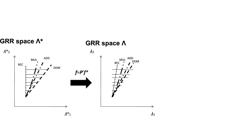
Figure 1: Plots of the GRR spaces $\Lambda^{*}$ and $\lambda$ under the inperfect LD model.

2.4 Properties of Genetic Models under the Imperfect LD Model

We defined genetic models using penetrances $(f_{0},\break f_{1},f_{2})$ at the SNP of interest. Under the imperfect LD model, the genetic model should be defined at the functional locus using $(f^{*}_{0},f^{*}_{1},f^{*}_{2})$. Thus, the REC, ADD, MUL or DOM models correspond to $\lambda^{*}_{1}=1$, $\lambda^{*}_{1}=(\lambda^{*}_{2}+1)/2$, $\lambda^{*}_{1}=\lambda^{*1/2}_{2}$, or $\lambda^{*}_{1}=\lambda^{*}_{2}$, respectively. A constrained family of possible genetic models at the functional locus is given by

$$\Lambda^{*}=\{(\lambda^{*}_{1},\lambda^{*}_{2})\dvtx\lambda^{*}_{2}\geq\lambda^{*}_{1}\mbox{ and }\lambda^{*}_{2}>1\}.$$ (4)

Note that $\Lambda$ and $\Lambda^{*}$ are different under the imperfect LD model, and they are linked by the two transition matrices in (2) and (3). Under the imperfect LD model, applying Table 2 to $f_{i}=\sum_{j=0}^{2}\operatorname{Pr}(G^{*}_{j}|G_{i})f^{*}_{j}$, we have

$$\qquad f_{0} = f^{*}_{0}(F_{1}^{2}+2F_{1}F_{3}\lambda^{*}_{1}+F_{3}^{2}\lambda^{*}_{2}),$$ (5)

$$f_{1} = f^{*}_{0}\{F_{1}F_{2}+(F_{1}F_{4}+F_{2}F_{3})\lambda^{*}_{1}+F_{3}F_{4}\lambda^{*}_{2}\},$$ (6)

$$f_{2} = f^{*}_{0}(F_{2}^{2}+2F_{2}F_{4}\lambda^{*}_{1}+F_{4}^{2}\lambda^{*}_{2}).$$ (7)

The true disease model at the functional locus, defined using $(\lambda^{*}_{1},\lambda^{*}_{2})$, is unknown. We study properties of the penetrances $(f_{0},f_{1},f_{2})$ or GRRs $(\lambda_{1},\lambda_{2})$ defined at the SNP given $(\lambda^{*}_{1},\lambda^{*}_{2})$.

Theorem 1.

Under the imperfect LD model with $|D^{\prime}|<1$, if $(\lambda^{*}_{1},\lambda^{*}_{2})\in\Lambda^{*}$ at the functional locus, then $(\lambda_{1},\lambda_{2})\in\Lambda$ at the marker locus. Moreover, for $(\lambda^{*}_{1},\lambda^{*}_{2})\in\Lambda^{*}-\{(1,1)\}$, if $\lambda^{*}_{1}=1$ (or $\lambda^{*}_{1}=\lambda^{*}_{2}$), then $\lambda_{1}>1$ (or $\lambda_{2}>\lambda_{1}$).

Using $F_{2}-F_{1}=-D/(pp_{c})=-(F_{4}-F_{3})$ and (5) to (7), we obtain

$$f_{1}-f_{0} = \frac{f^{*}_{0}D}{pp_{c}}\{F_{1}(\lambda^{*}_{1}-1)+F_{3}(\lambda^{*}_{2}-\lambda^{*}_{1})\},$$ (8)

$$f_{2}-f_{1} = \frac{f^{*}_{0}D}{pp_{c}}\{F_{2}(\lambda^{*}_{1}-1)+F_{4}(\lambda^{*}_{2}-\lambda^{*}_{1})\}.$$ (9)

It follows that $f_{2}\geq f_{1}\geq f_{0}$ and $f_{2}>f_{0}$ when $f^{*}_{2}\geq f^{*}_{1}\geq f^{*}_{0}$ and $f^{*}_{2}>f^{*}_{0}$. The proof of the second claim is trivial using the above two expressions and that, from Table 1, all $F_{i}$, $i=1,2,3,4$, are positive.

Theorem 1 shows that when the GRRs are constrained in $\Lambda^{*}$ at the functional locus, they are also constrained to a subset of $\Lambda$ at the SNP when $|D^{\prime}|<1$. In addition, when the true disease model is either REC or DOM at the functional locus, it is no longer REC or DOM at the SNP, respectively. They are “closer” to the ADD/MUL models. The implication of this finding is that one will not see a pure DOM or REC model at the marker locus if the constrained model space $\Lambda^{*}$ is considered at the functional locus. It also provides a rationale for the genetic model selection approach (Zheng and Ng, 2008) in that an ADD/MUL is always chosen unless there is strong evidence to indicate the REC or DOM models.

Even though the REC (or DOM) model at the functional locus is no longer retained at the SNP when $|D^{\prime}|<1$, the ADD (or MUL) model is retained. Dividing (8) and (9) by $f_{0}$, we obtain

$$2\lambda_{1}-1-\lambda_{2}=\frac{f^{*}_{0}D^{2}}{f_{0}p^{2}p_{c}^{2}}(2\lambda^{*}_{1}-1-\lambda^{*}_{2}).$$ (10)

Using (5) to (7) to expand $\lambda_{2}-\lambda^{2}_{1}=(f_{2}f_{0}-f_{1}^{2})/f^{2}_{0}$ and $(F_{2}F_{3}-F_{1}F_{4})^{2}=D^{2}/(p^{2}p^{2}_{c})$, we obtain

$$\lambda_{2}-\lambda^{2}_{1}=\frac{f^{*2}_{0}D^{2}}{f^{2}_{0}p^{2}p_{c}^{2}}(\lambda^{*}_{2}-\lambda^{*2}_{1}).\\$$ (11)

The above two equations lead directly to the following result.

Theorem 2.

Under the imperfect LD model with $|D^{\prime}|<1$, when the genetic model is ADD ($\lambda^{*}_{1}=(1+\lambda^{*}_{2})/2$) or MUL ($\lambda^{*}_{2}=\lambda^{*2}_{1}$) at the functional locus, the same model is retained at the marker locus.

Figure 1 displays the mapping of genetic models from $\Lambda^{*}$ to $\Lambda$ under the imperfect LD model. If we still define a genetic model at the marker locus under the imperfect LD model, then, using (3) and a table similar to Table 2, the REC or DOM models at the marker locus would correspond to the underdominant or overdominant models at the functional locus, respectively.

3 The Hardy–Weinberg Disequilibrium Coefficient and Genetic Model Selection

The Hardy–Weinberg disequilibrium (HWD) coefficient in cases or between cases and controls has been used to detect association (Nielsen, Ehm and Weir, 1998; Zaykin and Nielsen, 2000; Song and Elston, 2006). In addition, it can also be used to detect the underlying genetic model at the marker locus (Wittke-Thompson, Pluzhnikov and Cox, 2005; Zheng and Ng, 2008). In this section we first review the HWD coefficient and how it can be used to detect the genetic model at the SNP of interest. Then we study whether it can still be used to detect the genetic model which is defined at the functional locus under the imperfect LD model.

Using the notation in Section 1, the HWD coefficient at the SNP with alleles $A$ and $B$ is given by (Weir, 1996)

$$\Delta = \operatorname{Pr}(AA)-\{\operatorname{Pr}(AA)+\operatorname{Pr}(AB)/2\}^{2}$$

$$= g_{2}-(g_{2}+g_{1}/2)^{2}.$$

In cases and controls, it is denoted by $\Delta_{1}$ and $\Delta_{0}$, respectively, and given by

$$\Delta_{1} = p_{2}-(p_{2}+p_{1}/2)^{2}\quad\mbox{and}$$

$$\Delta_{0} = q_{2}-(q_{2}+q_{1}/2)^{2}.$$

Substituting $p_{i}=g_{i}f_{i}/k$ and $q_{i}=g_{i}(1-f_{i})/(1-k)$ under the Hardy–Weinberg proportions ($\Delta=0$), one has (Wittke-Thompson, Pluzhnikov and Cox, 2005; Zheng and Ng, 2008)

$$\hskip 25.0pt\Delta_{1} = \frac{f^{2}_{0}p^{2}p^{2}_{c}}{k^{2}}(\lambda_{2}-\lambda^{2}_{1}),$$ (12)

$$\Delta_{0} = \frac{f^{2}_{0}p^{2}p^{2}_{c}}{(1-k)^{2}}(2\lambda_{1}-1-\lambda_{2}-f_{0}\lambda^{2}_{1}+f_{0}\lambda_{2}).$$ (13)

Using the signs of $(\Delta_{1},\Delta_{0})$, Zheng and Ng (2008) divided $\Lambda$ in (1) into four mutually exclusive regions $R_{1}$ to $R_{4}$. The signs in the four regions are $(\Delta_{1},\Delta_{0})=(+,-)$ in $R_{1}$, $(-,-)$ in $R_{2}$, $(-,-)$ in $R_{3}$, and $(-,+)$ in $R_{4}$. The REC model belongs to $R_{1}$ and the DOM model belongs to $R_{4}$. The region $R_{2}$ is bounded by the ADD and MUL models (see Figure 1 of Zheng and Ng, 2008). Therefore, under the REC model (defined at the SNP with $\lambda_{1}=1$), $\Delta_{1}>0$ and $\Delta_{0}<0$, and under the DOM model, $\Delta_{1}<0$ and $\Delta_{0}>0$. Zheng and Ng (2008) used $\partial\Delta=\Delta_{1}-\Delta_{0}$ as a genetic model indicator. The REC model implies that $\partial\Delta>0$, while the DOM model implies $\partial\Delta<0$. A normalized test statistic based on $\widehat{\partial\Delta}=\widehat{\Delta}_{1}-\widehat{\Delta}_{0}$, where $\widehat{p}_{i}=r_{i}/r$ and $\widehat{q}_{i}=s_{i}/s$, is given

$$Z_{\mathrm{HWDTT}} = \frac{(rs/n)^{{1}/{2}}\widehat{\partial\Delta}}{\{1-n_{2}/n-n_{1}/(2n)\}\{n_{2}/n+n_{1}/(2n)\}}$$

$$\sim N(0,1)$$

under $H_{0}$ and referred to as the HWD trend test (HWDTT) (Song and Elston, 2006). It is used to select a genetic model (Zheng and Ng, 2008). Given that $B$ is the risk allele, the ADD (or MUL) model is chosen unless there is strong evidence to indicate a REC model or a DOM model. When $Z_{\mathrm{HWDTT}}>1.645$, the REC model is selected; when $Z_{\mathrm{HWDTT}}<-1.645$, the DOM model is selected.

Under the imperfect LD model, using (11) and (10), (12) and (13) can be written as

$$\Delta_{1} = \frac{f^{*2}_{0}D^{2}}{k^{2}}(\lambda^{*}_{2}-\lambda^{*2}_{1}),$$

$$\Delta_{0} = \frac{f_{0}f^{*}_{0}D^{2}}{(1-k)^{2}}(2\lambda^{*}_{1}-1-\lambda^{*}_{2}-f^{*}_{0}\lambda^{*2}_{1}+f^{*}_{0}\lambda^{*}_{2}).$$

Comparing the above $(\Delta_{1},\Delta_{0})$ with (12) and (13), we see that the signs of $(\Delta_{1},\Delta_{0})$ do not change when the genetic model is defined at the functional locus. Hence, the model selection procedure of Zheng and Ng (2008) can still be used.

4 Robust Tests

4.1 Pearson’s Test and CATTs

Given the case-control data for a single SNP, $(r_{0},\break r_{1},r_{2})$ and $(s_{0},s_{1},s_{2})$, denote $n_{i}=r_{i}+s_{i}$ for $i=0,1,2$ and $n=n_{0}+n_{1}+n_{2}$. Pearson’s test can be written as

$$T_{\chi^{2}} = \sum_{i=0}^{2}(r_{i}-n_{i}r/n)^{2}/(n_{i}r/n)$$

$${}+\sum_{i=0}^{2}(s_{i}-n_{i}s/n)^{2}/(n_{i}s/n),$$

which asymptotically follows a chi-squared distribution with 2 degrees of freedom (df) under $H_{0}$. The CATT with a score $x\in[0,1]$ is given by

$$Z_{x} = n^{1/2}\Biggl{(}n\sum_{j=0}^{2}x_{j}r_{j}-r\sum_{j=0}^{2}x_{j}n_{j}\Biggr{)}$$

$${}\Big{/}[rs\{n(n_{1}+4n_{2})-(n_{1}+2n_{2})^{2}\}]^{1/2},$$

where $(x_{0},x_{1},x_{2})=(0,x,1)$. Under $H_{0}$, $Z_{x}$ asymptotically follows the standard normal distribution $N(0,1)$ for a given $x$. Optimal scores for REC,ADD/MUL and DOM models are $x=0,1/2$ and $1$.

When the genetic model is unknown, $Z_{1/2}$ is often used. There is a trade-off between $T_{\chi^{2}}$ and $Z_{x}$ with $x=1/2$. Pearson’s test is more robust but less powerful, in particular, under the ADD or DOM models, while the trend test is more powerful under the ADD or DOM models but less robust when the score $x$ is misspecified. Pearson’s test is identical to the trend test $Z^{2}_{x}$ with $x=(r_{1}/n_{1}-r_{0}/n_{0})/(s_{1}/n_{1}-s_{0}/n_{0})$ (Yamada and Okada, 2009; Zheng, Joo and Yang, 2009). In practice, however, $x$ is prespecified. Thus, this condition is rarely satisfied.

4.2 MAX

To avoid the trade-off between Pearson’s test and the CATT, one approach is to consider maximum tests. A typical maximum test is given by (Freidlin et al., 2002; Sladek et al., 2007)

$$\mbox{MAX}_{3}=\max\{|Z_{0}|,|Z_{1/2}|,|Z_{1}|\}.$$

Other versions of maximum tests are also used, for example, $\mbox{MAX}=\sup_{x\in[0,1]}|Z_{x}|$ (Davies, 1977, 1987), the maximum of three likelihood ratio tests under various genetic models (González et al., 2008), and for a quantitative trait (Lettre, Lange and Hirschhorn, 2007).

Computational aspects of maximum tests have been discussed by Conneely and Boehnke (2007) and Li et al. (2008a). The empirical distribution of $\mbox{MAX}_{3}$ can be obtained from simulation using the joint multivariate normal distribution of the CATTs considering asymptotic null correlations among them (Freidlin et al., 2002) or from a parametric bootstrap procedure by generating data using $(r_{0},r_{1},r_{2})\sim\break\operatorname{Mul}(r;\widehat{p}_{0},\widehat{p}_{1},\widehat{p}_{2})$ and $(s_{0},s_{1},s_{2})\sim\operatorname{Mul}(s;\widehat{p}_{0},\widehat{p}_{1},\widehat{p}_{2})$, where $\widehat{p}_{i}=n_{i}/n$. A simpler algorithm to find the asymptotic and empirical null distributions of $\mbox{MAX}_{3}$ is recently proposed (Zang, Fung and Zheng, 2010). The asymptotic null distribution of $\mbox{MAX}_{3}$ is a function of the minor allele frequency (MAF) of the SNP. In a genome-wide scan to rank a large number of SNPs, Li et al. (2008b) demonstrated that ranking can be done easily by the values of $\mbox{MAX}_{3}$ rather than by their $p$-values. Hence, there is no need to calculate the $p$-values of $\mbox{MAX}_{3}$, even though the $p$-values of $\mbox{MAX}_{3}$ are more comparable across SNPs.

4.3 MIN2

An alternative approach used by WTCCC (2007) utilizes both Pearson’s test and the CATT $Z_{1/2}$. WTCCC (2007) proposed to use the minimum of the $p$-values of $T_{\chi^{2}}$ and $Z_{1/2}$ to scan all the SNPs. SNPs with the minimum $p$-value less than a threshold level were retained for further analyses. Joo et al. (2009) denoted the minimum of the two $p$-values by

$$\mbox{MIN2}=\min\{p_{T_{\chi^{2}}},p_{Z_{1/2}}\}$$

and obtained its asymptotic null distribution and its $p$-value, denoted by $p_{\mathrm{MIN2}}$. The key formula to find the distribution and $p$-value for MIN2 is the joint distribution of Pearson’s test and $Z_{1/2}$ under $H_{0}$, which is given by (Joo et al., 2009)

$$\operatorname{Pr}(Z^{2}_{1/2}<t_{1},T_{\chi^{2}}<t_{2})$$

$$\quad=1-\frac{1}{2}e^{-{t_{1}}/{2}}-{1}/{2}e^{-{t_{2}}{/2}}$$

$$\qquad{}+\frac{1}{2\pi}\int_{t_{1}}^{t_{2}}e^{-{v}/{2}}\arcsin\biggl{(}\frac{2t_{1}}{v}-1\biggr{)}\,dv,$$

when $t_{1}<t_{2}$, and $\operatorname{Pr}(Z^{2}_{1/2}<t_{1},T_{\chi^{2}}<t_{2})=1-\break\exp(-t_{2}/2)$ when $t_{1}>t_{2}$. Unlike $\mbox{MAX}_{3}$, the asymptotic null distribution of MIN2 does not depend on the MAFs of SNPs. Hence, MIN2 itself can be used to rank all SNPs, which results in the same ranks as when the $p$-value of MIN2 is used. Joo et al. (2009) demonstrated that $p_{\mathrm{MIN2}}>\mathrm{MIN2}$, because $Z^{2}_{1/2}$ and $T_{\chi^{2}}$ are correlated under the alternative hypothesis. Thus, MIN2 itself cannot be used as the $p$-value.

4.4 The Genetic Model Selection (GMS) Procedure

The GMS procedure is an adaptive approach. It contains two phases. In phase 1 the underlying genetic model is detected using the value and sign of $Z_{\mathrm{HWDTT}}$ (Song and Elston, 2006; see also Section 3). Once the model is selected (REC, ADD/MUL or DOM), in the second phase, the CATT optimal for the selected model is applied to test for association. For example, if the REC model is selected using the HWDTT, $Z_{0}$ would be used in phase 2 to test for association. Since the analyses in the two phases are correlated, Zheng and Ng (2008) derived the asymptotic null correlation for the GMS. This correlation is incorporated in the distribution of the test statistics to control for the Type I error. Like MIN2, computing the $p$-value of the GMS requires integrations. Like $\mbox{MAX}_{3}$, the GMS can be used to rank SNPs (Zheng et al., 2009). Using test statistics to directly rank SNPs is easier than using $p$-values of the GMS. Since the GMS depends on which allele is the risk allele or whether the minor allele is the risk allele, for each SNP, we first determine the risk allele ($B$ is risk allele if $Z_{1/2}>0$). If the risk allele is $B$, then the above GMS can be applied. Otherwise, we can switch the two alleles and apply the above GMS.

4.5 Other Tests

Balding (2006) provided an excellent review of statistical methods for the analysis of association studies. Two other robust two-phase tests are also available that we do not include here. One feature of these methods is that the test statistics in two phases are asymptotically independent under $H_{0}$(Zheng, Song and Elston, 2007, Zheng et al., 2008). In this case, the second phase can be used as a “self-replication,” an idea proposed in van Steen et al. (2005). Alternatively, the significance level $\alpha$ can be decomposed to $(\alpha_{1},\alpha_{2})$ such that $\alpha_{1}\alpha_{2}=\alpha$, where $\alpha_{1}$ is used for the phase 1 analysis and $\alpha_{2}$ for the phase 2 analysis. The null hypothesis is rejected when analyses in both phases are significant at their corresponding levels. Choices of $\alpha_{1}$ and $\alpha_{2}$ with $\alpha_{1}\alpha=\alpha$ in GWAS were discussed in Zheng, Song and Elston (2007), Zheng et al. (2008). Another robust test is the constrained likelihood ratio test (LRT) (Wang and Sheffield, 2005). It is similar to the LRT except that the alternative space is restricted to $\Lambda-\{(1,1)\}$. The performance of the constrained LRT is similar to that of $\mathrm{MAX}_{3}$ described above. Thus, we only consider $\mathrm{MAX}_{3}$ here.

4.6 Why Robust Tests?

One of the reasons that we use robust tests in GWAS is that there might be multiple functional loci for a given disease. The modes of inheritance or genetic models may differ from one functional locus to the other. Another reason for using robust tests is the distortion of the actual genetic model at the marker locus due to incomplete LD, which further amplifies uncertainty about the model. Thus, robust tests are generally preferred. We use efficiency robustness to measure robustness (Gastwirth, 1985). A test $T_{1}$ is said to have greater efficiency robustness than a test $T_{2}$ if the worst asymptotic relative efficiency of $T_{1}$ to the asymptotically optimal test across all genetic models is higher than the worst asymptotic relative efficiency of $T_{2}$. The CATT $Z_{1/2}$ optimal for the ADD model is most robust among all trend tests when the genetic models are constrained in $\Lambda$. Pearson’s test is also robust because it does not require the genetic models to be constrained or the alternative hypothesis to be ordered. When restricting to $\Lambda$, tests more robust than $Z_{1/2}$ are available. $\mbox{MAX}_{3}$ and GMS are two examples. They both have greater efficiency robustness than Pearson’s test and $Z_{1/2}$ (Freidlin et al., 2002; Zheng and Ng, 2008). On the other hand, combining information of both Pearson’s test and $Z_{1/2}$, MIN2 is also more efficiency robust than either Pearson’s test or $Z_{1/2}$. Three robust tests, $\mbox{MAX}_{3}$, GMS and MIN2, appear to have comparable efficiency robustness in candidate-gene studies (Joo et al., 2009).

In genome-wide scans it is desirable to locate the SNPs representing true association as near the top as possible, where all SNPs compete for the top ranks. Under the complete LD model, Zheng et al. (2009) conducted simulation studies comparing the three robust methods in ranking 300,000 SNPs,among which there were 6 functional loci with different genetic models, MAFs and GRRs (from 1.25 to 1.5). The results showed that the GMS slightly outperforms MIN2 and $\mbox{MAX}_{3}$ when the top 5000 SNPs were selected. The criteria used for comparison included the probability that the top 5000 SNPs contained at least one SNP with true association, as well as the minimum and average ranks of SNPs with true associations among the top 5000 SNPs. We will conduct similar simulation studies in Section 5 under the inperfect LD model. The reason that we choose the top 5000 SNPs rather than a smaller number, say, the top 100, is that the SNPs with true association are not always ranked near the top, especially for a small GRR between 1.2 and 1.5 and small sample sizes (Zaykin and Zhivotovsky, 2005). If we examine the top 100 list with 250 cases and 250 controls (the sample sizes that we used in our simulation studies), the probability that the list of the top 100 SNPs contains a true association is less than 0.50.

5 Simulation Studies

5.1 The GMS Procedure under the Imperfect LD Model

We first conducted simulation studies to estimate the distribution of genetic models selected by the GMS. We chose disease prevalence $k=0.1$ and GRR $\lambda^{*}_{2}=2$ at the functional locus. Then $\lambda^{*}_{1}$ was obtained using $\lambda^{*}_{2}$ and a given genetic model at the functional locus. We considered 0.1, 0.3 and 0.5 for the equal MAFs at a SNP ($p$) and a functional locus ($q$). This allows us to compare the frequencies of the different models selected when $D^{\prime}=1.0$, 0.8 and 0.6. With equal allele frequencies $p=q$, Corr$(A,a)=D^{\prime}$. In each of 10,000 replicates, 250 cases and 250 controls were simulated from multinomial distributions in which the penetrances at a SNP were calculated using (5) to (7). When the GMS did not select REC or DOM, the ADD or MUL models are used and denoted here by A/M. Results are reported in Table 3.

Table 3: Distributions of genetic models selected by the GMS using the HWDTT (%): Disease prevalence $k=0.1$, the GRR at the functional locus $\lambda^{*}_{2}=2$ with 250 cases and 250 controls and 10,000 replicates

		$\bolds{D^{\prime}}$/selected models (A/M $\bolds{=}$ ADD/MUL)
3-11
		1.0			0.8			0.6
3-5,6-8,9-11
MAF $\bolds{p=q}$	True model	REC	A/M	DOM	REC	A/M	DOM	REC	A/M	DOM
0.1	REC	$23.3$	$76.3$	$0.4$	$14.6$	$84.4$	$1.0$	$3.0$	$90.6$	$6.4$
	ADD	$2.6$	$88.9$	$8.5$	$2.4$	$90.2$	$7.4$	$2.9$	$90.8$	$6.3$
	MUL	$3.4$	$90.3$	$6.3$	$3.7$	$91.1$	$5.2$	$3.8$	$90.8$	$5.4$
	DOM	$0.1$	$60.1$	$39.8$	$0.3$	$76.1$	$23.6$	$1.0$	$84.8$	$14.2$
0.3	REC	$67.5$	$32.5$	$0.0$	$39.4$	$60.4$	$0.2$	$18.6$	$80.6$	$0.8$
	ADD	$2.2$	$88.9$	$8.9$	$3.1$	$89.3$	$7.6$	$3.7$	$89.6$	$6.7$
	MUL	$4.8$	$90.7$	$4.5$	$5.0$	$90.4$	$4.6$	$5.2$	$90.1$	$4.7$
	DOM	$0.0$	$32.8$	$67.2$	$0.1$	$61.4$	$38.5$	$0.7$	$80.2$	$19.1$
0.5	REC	$66.0$	$34.0$	$0.0$	$36.8$	$63.1$	$0.2$	$18.3$	$80.9$	$0.8$
	ADD	$2.6$	$89.0$	$8.4$	$3.3$	$89.6$	$7.1$	$3.7$	$90.8$	$5.5$
	MUL	$5.4$	$89.9$	$4.7$	$5.0$	$90.1$	$4.9$	$5.2$	$89.9$	$4.9$
	DOM	$0.0$	$36.2$	$63.8$	$0.1$	$63.9$	$36.0$	$0.8$	$81.2$	$18.0$

When the true model is REC or DOM at the functional locus, the frequencies that the model selected by the GMS at the marker locus is REC or DOM decreases dramatically when $D^{\prime}$ becomes small. For example, when $p=q=0.3$, the frequency of selecting REC at the marker locus is about 67.5% when the true model at the functional locus is REC, and $D^{\prime}=1$. This frequency declines to 18.6% when $D^{\prime}=0.6$. These frequencies, however, are not sensitive when the true model at the functional locus is either ADD or MUL. The findings are consistent with Theorems 1 and 2. Given the genetic model space $\Lambda^{*}$ at the functional locus, the genetic model space at the marker locus $\Lambda$ is shifted toward the center of the space $\Lambda^{*}$ corresponding to the ADD/MUL models.

Table 4: GRRs $(\lambda_{1},\lambda_{2})$ at a SNP given GRR $\lambda^{*}_{2}=2$ at the functional locus: $p=q=0.3$. When $D^{\prime}=1$, $\lambda^{*}_{i}=\lambda_{i}$ for $i=1,2$

	$\bolds{D^{\prime}/(\lambda_{1},\lambda_{2})}$
2-4
True model	1.0	0.8	0.6
REC	(1.00, 2.00)	(1.05, 1.73)	(1.07, 1.50)
ADD	(1.50, 2.00)	(1.38, 1.75)	(1.27, 1.54)
MUL	(1.41, 2.00)	(1.22, 1.48)	(1.24, 1.53)
DOM	(2.00, 2.00)	(1.67, 1.77)	(1.43, 1.57)

Table 4 reported the GRRs at the marker locus given those at the functional locus. Note that when the true model is ADD ($\lambda^{*}_{1}=(1+\lambda^{*}_{2})/2$) or MUL ($\lambda^{*2}_{1}=\lambda^{*}_{2}$), the GRRs at the marker locus follow the same models. However, $\lambda_{i}$ are smaller than $\lambda^{*}_{i}$. Similar patterns are observed when the true model is REC or DOM, except that $\lambda_{1}$ is slightly greater than $\lambda^{*}_{1}$ under the REC model.

5.2 Comparison of Robust Tests in GWAS under the Imperfect LD Model

In Table 3 when the true model is REC or DOM at the functional locus, the GMS could not select REC or DOM at the marker locus. This, however, does not mean that the GMS cannot improve power or chances of true discoveries when $|\operatorname{Corr}(A,a)|<1$. On the contrary, owing to the shrinkage of the genetic model space and that the GMS only selects a model at the marker locus, it can be viewed as selecting an appropriately induced model at the marker locus. Our next simulation will examine the performance of robust tests under the imperfect LD model. The simulation procedure follows the one used in Zheng et al. (2009). We simulated genotype counts for each of 300,000 SNPs, among which 6 SNPs have true associations and $D^{\prime}=0.8$ with MAF of 0.2 at the functional loci. When $D^{\prime}=1$, the number of functional loci is also 6. However, when $D^{\prime}=0.8$, we assume the number of functional loci equals the number of different genetic models in the simulation. Zheng et al. (2009) considered the perfect LD model that corresponds to $|D^{\prime}|=1$ or $|\operatorname{Corr}(A,a)|=1$. Their results are repeated here for comparison. The MAFs of 6 true SNPs from the genetic models listed in the titles of Tables 5 and 6 were 0.1821, 0.2943, 0.1078, 0.4459, 0.1620 and 0.1825. These are also given in Zheng et al. (2009) and in Li et al. (2008b). MAFs for the rest of the null SNPs were simulated from a uniform distribution $U(0.1,0.5)$. The GRRs for the functional loci were all 1.25 (or 1.50). We applied five robust tests ($Z_{1/2}$, Pearson’s test $T_{\chi^{2}}$, GMS, MIN2 and $\mbox{MAX}_{3}$) to rank all SNPs and the top 5000 SNPs were selected from each of 200 replicates. The criteria to compare the performance of robust tests include the probability (prob %) of at least one true SNP being selected among the top 5000 SNPs, the average number of true SNPs among the top, and the mean of the minimum ranks of the true SNPs among the top. The results are presented in Table 5 (2 REC, 1 ADD, 1 MUL and 2 DOM SNPs) and Table 6 (1 REC, 2 ADD, 2 MUL and 1 DOM SNPs).

First, when $D^{\prime}=1$ (Zheng et al., 2009), the GMS outperforms other tests under all three criteria, while Pearson’s test had the worst performance. When $D^{\prime}=0.8$, however, the GMS and $Z_{1/2}$ had similar performances, which together outperform other tests using the three criteria. This finding is consistent to our results in Theorems 1 and 2 about the genetic models under the imperfect LD model.

Table 5: Genome-wide scans of 300,000 SNPs containing 6 true SNPs (2 REC, 1 ADD, 1 MUL and 2 DOM). Only the top 5000 SNPs are selected. The results are based on 200 replicates: MAF $q=0.2$ at the functional locus when $D^{\prime}=0.8$. Samples sizes are $r=s=1000$ for GRR=1.25 and $r=s=500$ for GRR=1.5

		$\bolds{D^{\prime}=1.0}$			$\bolds{D^{\prime}=0.8}$
3-5,6-8
GRR $\bolds{\lambda_{2}}$	Robust tests	Prob	Ave. no. of true SNPs	Mean of min ranks	Prob	Ave. no. of true SNPs	Mean of min ranks
1.25	$Z_{1/2}$	$92.0$	1.79	971	58.5	1.29	1625
	GMS	$94.5$	1.90	838	56.0	1.29	1488
	$\mbox{MAX}_{3}$	$90.5$	1.80	909	48.0	1.28	1435
	MIN2	$89.5$	1.79	934	51.0	1.25	1550
	$T_{\chi^{2}}$	$86.5$	1.69	960	46.5	1.22	1680
1.50	$Z_{1/2}$	$99.5$	2.71	186	83.0	1.49	1041
	GMS	$100.0$	2.99	178	85.0	1.54	1111
	$\mbox{MAX}_{3}$	$99.5$	2.83	205	80.0	1.48	1183
	MIN2	$100.0$	2.78	234	80.0	1.50	1113
	$T_{\chi^{2}}$	$100.0$	2.71	286	75.0	1.46	1244

Table 6: Genome-wide scans of 300,000 SNPs containing 6 true SNPs (1 REC, 2 ADD, 2 MUL and 1 DOM). Only the top 5000 SNPs are selected. The results are based on 200 replicates: MAF $q=0.2$ at the functional locus and $D^{\prime}=0.8$. Samples sizes are $r=s=1000$ for GRR=1.25 and $r=s=500$ for GRR=1.5

		$\bolds{D^{\prime}=1.0}$			$\bolds{D^{\prime}=0.8}$
3-5,6-8
GRR $\bolds{\lambda_{2}}$	Robust tests	Prob	Ave. no. of true SNPs	Mean of min ranks	Prob	Ave. no. of true SNPs	Mean of min ranks
1.25	$Z_{1/2}$	88.0	1.72	$897$	49.5	1.31	1564
	GMS	87.0	1.79	$797$	53.5	1.27	1630
	$\mbox{MAX}_{3}$	82.5	1.64	$846$	47.0	1.24	1702
	MIN2	86.0	1.66	$932$	48.5	1.25	1899
	$T_{\chi^{2}}$	83.0	1.50	$1030$	41.5	1.20	1847
1.50	$Z_{1/2}$	99.0	2.46	$349$	76.5	1.48	1083
	GMS	99.5	2.61	$355$	76.0	1.47	1005
	$\mbox{MAX}_{3}$	98.0	2.34	$379$	73.0	1.40	1103
	MIN2	99.5	2.35	$434$	74.0	1.38	1105
	$T_{\chi^{2}}$	97.0	2.21	$485$	66.5	1.31	1179

Table 7: Ranks of SNPs with strong association of seven diseases in WTCCC (2007), Table 3

Disease	SNP ID	chrom	$\bolds{Z_{1/2}}$	$\bolds{T_{\chi^{2}}}$	GMS	$\mathbf{MAX_{3}}$	MIN2
BD	rs420259	$16$	$269$	$22$	$19$	$20$	$23$
CAD	rs1333049	$9$	$9$	$25$	$24$	$24$	$25$
CD	rs11805303	$1$	$14$	$28$	$23$	$24$	$24$
	rs10210302	$2$	$6$	$15$	$15$	$16$	$15$
	rs9858542	$3$	$102$	$58$	$58$	$61$	$75$
	rs17234657	$5$	$11$	$25$	$19$	$20$	$21$
	rs1000113	$5$	$72$	$92$	$78$	$82$	$84$
	rs10761659	$10$	$89$	$115$	$100$	$107$	$101$
	rs10883365	$10$	$50$	$65$	$59$	$62$	$61$
	rs17221417	$16$	$25$	$37$	$35$	$37$	$38$
	rs2542151	$18$	$69$	$84$	$77$	$80$	$81$
RA	rs6679677	$1$	$50$	$72$	$71$	$69$	$70$
	rs6457617	$6$	$5$	$13$	$8$	$8$	$13$
T1D	rs6679677	$1$	$129$	$137$	$133$	$136$	$135$
	rs9272346	$6$	$3$	$6$	$5$	$5$	$5$
	rs11171739	$12$	$339$	$361$	$342$	$357$	$354$
	rs17696736	$12$	$233$	$245$	$238$	$243$	$242$
	rs12708716	$16$	$521$	$534$	$517$	$534$	$530$
T2D	rs9465871	$6$	$31$	$41$	$49$	$44$	$45$
	rs4506565	$10$	$10$	$17$	$17$	$17$	$16$
	rs9939609	$16$	$24$	$38$	$36$	$36$	$37$

6 Applications to WTCCC Data

We apply the five robust tests to a genome-wide scan using more than 300,000 SNPs after quality control. The study was originally conducted byWTCCC (2007) for seven diseases (type 1 diabetes—T1D, type 2 diabetes—T2D, coronary heart disease—CHD, hypertension—HT, bipolar disorder—BD,rheumatoid arthritis—RA and Crohn’s disease—CD). About 2000 cases were used for each disease and 3000 controls were shared for the seven diseases. WTCCC (2007) used MIN2 to test for association after the quality control. They obtained two tables presenting SNPs with strong associations with$\mathrm{MIN2}<5\times 10^{-7}$ (Table 3 of WTCCC, 2007) and SNPs with moderate associations with $5\times 10^{-7}\leq\mathrm{MIN2}<5\times 10^{-5}$ (Table 4 of WTCCC, 2007). We reanalyze these data by ranking all SNPs after our quality control. The goal of this application is to demonstrate the efficiency robustness of different test statistics, not to find SNPs with associations that were not reported in WTCCC (2007).

In our application, for each of the seven diseases, we rank all SNPs after quality control (398,092 SNPs) using the five robust tests and report the ranks of the SNPs that were reported to have strong associations in WTCCC (2007), Table 3. Note that we do not know $D^{\prime}$ in reality, nor do we know the number of functional loci and their modes of inheritance. Our results are reported in Table 7. The results show that SNPs with strong associations are all ranked on the top 5000 SNPs. The CATT is least robust among the five robust tests as shown by the rank 269 for BD, while the ranks by the other methods are less than 25. The GMS tends to have smaller ranks than $\mathrm{MAX}_{3}$, and MIN2 tends to have ranks between the CATT and Pearson’s test, which often have higher ranks than the GMS.

We also studied the ranks of SNPs with moderate associations reported in WTCCC (2007), Table 4. The detailed results are not shown here, but summarized below. Similar patterns are also observed, although, for several SNPs, the CATT has large ranks. For example, for BD, the CATT has rank 147,769 for SNP rs6458307 on chromosome 6, while the ranks of other tests for this SNP are less than 150. For T2D, the CATT has rank 197,064 for SNP rs358806 on chromosome 3, while the other tests have ranks less than 100. All ranks of SNPs with either strong or moderate associations are less than 5000, and only one SNP (rs17166496 for T1D on chromosome 5) is ranked more than 5000 by $\mathrm{MAX}_{3}$ and the GMS. The actual ranks for this SNP are 5521 for the GMS and 6063 for $\mathrm{MAX}_{3}$, 652 for Pearson’s test, 724 for MIN2, but 245,454 for the CATT. The underlying genetic model for this SNP could be outside of the constrained genetic model that we considered here, for example, overdominant or underdominant for which it is known that Pearson’s test is robust (Zheng, Joo and Yang, 2009; Joo et al., 2009). In addition, we found that for those SNPs with small ranks based on Pearson’s test, a large rank using the CATT is always accompanied by a large value of the HWDTT. This is due to the orthogonal decomposition of Pearson’s test to the HWDTT and $Z_{1/2}^{2}$ (Zheng et al., 2008). It is also interesting to note that, even if a SNP has a rank smaller than those SNPs listed in Table 7, it does not mean the SNP has a true association with a disease. That is, in GWAS, a SNP with smaller $p$-value does not necessarily mean it has stronger association. In fact, many of these SNPs with smaller ranks have not been confirmed to have true associations (WTCCC, 2007). This is because a very small number of SNPs ($<$100 SNPs) are associated with a disease in GWAS compared to the number of null SNPs (more than 300,000 SNPs). Therefore, the probability that test statistics of some null SNPs are greater than those of all the associated SNPs is high (Zaykin and Zhivotovsky, 2005).

7 Discussion

We studied some robust tests for case-control genetic association studies. This approach stems from the classical robust procedures studied in the 1970s which focused on the estimation of the location parameter of a symmetric distribution. For a given family of underlying distributions (or, here, genetic models), an estimate with a high (low) minimum correlation, say, $>$0.80 ($<$0.50) with the optimal procedure, indicates a greater (smaller) efficiency robustness. In early work, the underlying distribution was assumed to range from the normal distribution to the Cauchy distribution (Tukey, 1965 and Andrews et al., 1965). For this family of $t$-distributions, the robust estimate of the location parameter was considered, because within the family of distributions considered, it had minimum correlation with the optimal procedure of about 0.60 (Gastwirth,1966). In case-control genetic association studies, when the true genetic model is unknown and ranges from the REC to the DOM models, the minimum correlation of any two CATTs is about 0.30 (Freidlin et al., 2002). This indicates that using a single CATT for association is not robust, and tests that are robust across a family of plausible genetic models are preferred.

Previous studies of robustness properties of test statistics for the analysis of case-control genetic association studies have been focused on the perfect (or complete) LD model, that is, the genetic marker (SNP) is also the functional locus. In this article we studied genetic models under a general imperfect (or incomplete) LD model with linkage disequilibrium between linked marker locus and functional locus. The perfect LD model is a special case. Under the imperfect LD model, we found that a genetic model defined by the genotype relative risks at the functional locus usually no longer remains the same genetic model at the marker locus, except for the additive or multiplicative models. The genetic model space at the marker locus is a subset of that at the functional locus, resulting in smaller genotype relative risks at the marker than at the functional locus. The power to detect a true association is reduced when the linkage disequilibrium decreases, while the model uncertainty increases, complicating the choice of a single association statistic. Robust tests are shown to perform optimally in this situation.

We also review some common efficiency robust tests for case-control genetic associations and their usage in genome-wide scans. In genome-wide scans, all SNPs are ranked by a test statistic or its $p$-value (if the $p$-value is readily obtained) and the top-ranked SNPs are selected for further analyses. Alternatively, as in WTCCC (2007), some genome-wide threshold levels can be also used to select SNPs. Multiple testing is an important issue in GWAS not only because one tests 300,000 up to a million SNPs, but also because multiple tests are available for each SNP (and there is no uniform most powerful test in GWAS). Correcting for multiple testing remains challenging in the analysis of GWAS (Roeder and Wasserman, 2009), and the need for independent replication studies (Kraft, Zeggini and Ioannidis, 2009) and proper meta-analysis (Pfeiffer, Gail and Pee, 2009) cannot be overemphasized.

References

- (1) Andrews, D. F., Bickel, P. J., Hampel, F. R., Huber, P. J., Rogers, W. H. and Tukey, J. W. (1965). Robust Estimation of Location. Princeton Univ. Press, Princeton, NJ.
- (2) Balding, D. J. (2006). A tutorial on statistical methods for population association studies. Nat. Rev. Genet. 7 781–791.
- (3) Conneely, K. N. and Boehnke, M. (2007). So many correlated tests, so little time! Rapid adjustment of P values for multiple correlated tests. Am. J. Hum. Genet. 81 1158–1168.
- (4) Davies, R. B. (1977). Hypothesis testing when a nuisance parameter is present only under the alternative. Biometrika 64 247–254. \MR0501523
- (5) Davies, R. B. (1987). Hypothesis-testing when a nuisance parameter is present only under the alternative. Biometrika 74 33–43. \MR0885917
- (6) Elston R. C., Lin, D. Y. and Zheng, G. (2007). Multistage sampling for genetic studies. Ann. Rev. Gen. Hum. Genet. 8 327–342.
- (7) Freidlin, B., Zheng, G., Li, Z. and Gastwirth, J. L. (2002). Trend tests for case-control studies of genetic markers: Power, sample size and robustness. Hum. Hered. 53 146–152 (Erratum 68 (2009) 220).
- (8) Gail. M. H., Pfeiffer. R. M., Wheeler. W. and Pee, D. (2008). Probability of detecting disease-associated single nucleotide polymorphisms in case-control genome-wide association studies. Biostatistics 9 201–215.
- (9) Gastwirth, J. L. (1966). On robust procedures. J. Amer. Statist. Assoc. 61 929–948. \MR0205397
- (10) Gastwirth, J. L. (1985). The use of maximin efficiency robust tests in combining contingency tables and survival analysis. J. Amer. Statist. Assoc. 80 380–384. \MR0792737
- (11) González, J. R., Carrasco, J. L., Dudbridge, F., Armengol, L., Estivill, X. and Moreno, V. (2008). Maximizing association statistics over genetic models. Genet. Epidemiol. 32 246–254.
- (12) Guedj, M., Nuel, G. and Prum, B. (2008). A note on allelic tests in case-control association studies. Ann. Hum. Genet. 72 407–409.
- (13) Hanson, R. L., Looker, H. C., Ma, L., Muller, Y. L., Baier, L. J. and Knowler, W. C. (2006). Design and analysis of genetic association studies to finely map a locus identified by linkage analysis: Sample size and power calculations. Ann. Hum. Genet. 70 332–349.
- (14) Hoh, J. and Ott, J. (2003). Mathematical multi-locus approaches to localizing complex human trait genes. Nat. Rev. Genet. 4 701–709.
- (15) Joo, J., Kwak, M., Ahn, K. and Zheng, G. (2009). A robust genome-wide scan statistic of the Wellcome Trust Case-Control Consortium. Biometrics 65 1115–1122.
- (16) Klein, R. J., Zeiss, C., Chew, E. Y., Tsai, J. Y., Sackler, R. S., Haynes, C., Henning, A. K., SanGiovanni, J. P., Mane, S. M., Mayne, S. T., Bracken, M. B., Ferris, F. L., Ott, J., Barnstable, C. and Hoh, J. (2005). Complement factor H polymorphism in aged-related macular degeneration. Science 308 385–389.
- (17) Kraft, P., Zeggini, E. and Ioannidis, J. P. A. (2009). Replication in genome-wide association studies. Statist. Sci. 24 561–573.
- (18) Lettre, G., Lange, C. and Hirschhorn, J. N. (2007). Genetic model testing and statistical power in population-based association studies of quantitative traits. Genet. Epidemiol. 31 358–362.
- (19) Lewontin, R. C. (1964). The interaction of selection and linkage. I. General considerations; heterotic models. Genetics 49 49–67.
- (20) Li, Q., Zheng, G., Li, Z. and Yu, K. (2008a). Efficient approximation of P-value of the maximum of correlated tests, with applications to genome-wide association studies. Ann. Hum. Genet. 72 397–406.
- (21) Li, Q., Yu, K., Li, Z. and Zheng, G. (2008b). MAX-rank: A simple and robust genome-wide scan for case-control association studies. Hum. Genet. 123 617–623.
- (22) Marchini, J., Donnelly, P. and Cardon, L. R. (2005). Genome-wide strategies for detecting multiple loci that influence complex diseases. Nat. Genet. 37 413–417.
- (23) Nielsen, D. M., Ehm, M. G. and Weir, B. S. (1998). Detecting marker-disease association by testing for Hardy-Weinberg disequilibrium at a marker locus. Am. J. Hum. Genet. 63 1531–1540.
- (24) Nielsen, D. M. and Weir, B. S. (1999). A classical setting for associations between markers and loci affecting quantitative traits. Genet. Res. 74 271–277.
- (25) Pfeiffer, R. M., Gail, M. H. and Pee, D. (2009). On combining data from genome-wide association studies to discover disease-associated SNPs. Statist. Sci. 24 547–560.
- (26) Roeder, K. and Wasserman, L. (2009). Genome-wide significance levels and weighted hypothesis testing. Statist. Sci. 24 398–413.
- (27) Sasieni, P. D. (1997). From genotypes to genes: Doubling the sample size. Biometrics 53 1253–1261. \MR1614374
- (28) Schaid, D. J., McDonnell, S. K., Hebbring, S. J., Cunningham, J. M. and Thibodeau, S. N. (2005). Nonparametric tests of association of multiple genes with human diseases. Am. J. Hum. Genet. 76 780–793.
- (29) Sladek, R., Rocheleau, G., Rung, J., Dina, C., Shen, L. Serre, D., Boutin, P., Vincent, D., Belisle, A., Hadjadj, S., Balkau, B., Heude, B. et al. (2007). A genome-wide association study identifies novel risk loci for type 2 diabetes. Nature 445 881–885.
- (30) Song, K. and Elston, R. C. (2006). A powerful method of combining measures of association and Hardy-Weinberg disequilibrium for fine-mapping in case-control studies. Stat. Med. 25 105–126. \MR2222077
- (31) Thomas, D. C., Casey, G., Conti, D., Haile, R. W., Lewinger, J. P. and Stram, D. O. (2009). Methodological issues in multistage genome-wide association studies. Statist. Sci. 24 414–429.
- (32) Tukey, J. W. (1965). Which part of the sample contains the information? Proc. Natl. Acad. Sci. USA 53 127–134. \MR0172387
- (33) Van Steen, K., McQueen, M. B., Herbert, A., Raby, B., Lyon, H., DeMeo, D. L., Murphy, A., Su, J., Datta, S., Rosenow, C., Christman, M., Silverman, E. K., Laird, N. M., Weiss, S. T. and Lange, C. (2005). Genomic screening and replication using the same data set in family-based association testing. Nat. Genet. 37 683–691.
- (34) Wang, K. and Sheffield, V. C. (2005). A constrained-likelihood approach to marker-trait association studies. Am. J. Hum. Genet. 77 768–780.
- (35) Weir, B. S. (1996). Genetic Data Analysis II: Methods for Discrete Population Genetic Data. Sinauer, Sunderland, MA.
- (36) Wittke-Thompson, J. K., Pluzhnikov, A. and Cox, N. J. (2005). Rational inferences about departure from Hardy-Weinberg equilibrium. Am. J. Hum. Genet. 76 967–986.
- (37) The Wellcome Trust Case Control Consortium (WTCCC) (2007). Genome-wide association study of 14,000 cases of seven common diseases and 3,000 shared controls. Nature 447 661–678.
- (38) Yamada, R. and Okada, Y. (2009). An optimal dose-effect mode trend test for SNP genotype tables. Genet. Epidemiol. 33 114–127.
- (39) Zang, Y., Fung, W. K. and Zheng, G. (2010). Simple algorithms to calculate asymptotic null distributions for robust tests in case-control genetic association studies in R. J. Stat. Software 33 1–24.
- (40) Zaykin, D. V. and Nielsen, D. M. (2000). Hardy-Weinberg disequilibrium (HWD) fine mapping for case-control samples. Am. J. Hum. Genet. 67 1238 Suppl.
- (41) Zaykin, D. V. and Zhivotovsky, L. A. (2005). Ranks of genuine associations in whole-genome scans. Genetics 171 813–823.
- (42) Zheng, G. and Ng, H. K. T. (2008). Genetic model selection in two-phase analysis for case-control association studies. Biostatistics 9 391–399.
- (43) Zheng, G., Joo, J. and Yang, Y. (2009). Pearson’s test, trend tests and MAX are all trend tests with different types of scores. Ann. Hum. Genet. 73 133–140.
- (44) Zheng, G., Song, K. and Elston, R. C. (2007). Adaptive two-stage analysis of genetic association in case-control designs. Hum. Hered. 63 175–186.
- (45) Zheng, G., Meyer, M., Li, W. and Yang, Y. (2008). Comparison of two-phase analyses for case-control genetic association studies. Stat. Med. 27 5054–5075.
- (46) Zheng, G., Joo, J., Tian, X., Wu, C. O., Lin, J.-P., Stylianou, M., Waclawtw, M. A. and Geller N. L. (2009). Robust genome-wide scans with genetic model selection using case-control design. Stat. Interface (A special issue in honor of Joseph Gastwirth) 2 145–151. \MR2516065