Spatially heterogeneous dynamics in a thermosensitive soft suspension before and after the glass transition

Rémy Colin^a, Ahmed M. Alsayed^b, Jean-Christophe Castaing^b, Rajesh Goyal^b, Larry Hough^b and Bérengère Abou^a

The microscopic dynamics and aging of a soft thermosensitive suspension was investigated by looking at the thermal fluctuations of tracers in the suspension. Below and above the glass transition, the dense microgel particles suspension was found to develop an heterogeneous dynamics, featured by a non Gaussian Probability Distribution Function (PDF) of the probes’ displacements, with an exponential tail. We show that non Gaussian shapes are a characteristic of the ensemble-averaged PDF, while local PDF remain Gaussian. This shows that the scenario behind the non Gaussian van Hove functions is a spatially heterogeneous dynamics, characterized by a spatial distribution of locally homogeneous dynamical environments through the sample, on the considered time scales. We characterize these statistical distributions of dynamical environments, in the liquid, supercooled, and glass states, and show that it can explain the observed exponential tail of the van Hove functions observed in the concentrated states. The intensity of spatial heterogeneities was found to amplify with increasing volume fraction. In the aging regime, it tends to increase as the glass gets more arrested.

1 Introduction

Dense colloidal suspensions are a powerful model system to study the glass and jamming transitions. With increasing volume fraction, the suspension dynamics may experience a slowing down of several orders of magnitude, as well as a change of qualitative behaviour, from viscous to elastic, at reasonable experimental time scales, with no significant structural changes in the suspension^{1, 2}. This colloidal glass transition is analogous to the glass transition in liquids and polymer melts and to the jamming transition in granular materials³. Because the colloidal particles are larger than molecules, these systems provide slower accessible times scales than in atomic and molecular glasses, and the possibility to be probed with optical techniques including microscopy and dynamic light scattering⁴. Hard spheres suspensions have been extensively investigated for their relative simplicity in modelling the glass transition¹. Recently, soft colloidal suspensions have also attracted attention. They can be flexibly designed with various particles softness and interactions – attractive or repulsive – allowing for a wider variety of behaviour in mimicking the glass transition in traditional glasses⁵. One of the most investigated soft systems consists of aqueous suspensions of thermosensitive microgels, made with amphiphilic cross-linked poly(N-isopropylacrylamid) polymer (pNIPAm)⁶. These particles can be designed with various softnesses, depending on the cross-linkers density⁷. Moreover and not least, the particles radius in the suspension, and therefore their volume fraction, can be reversibly tuned with temperature, which provides a unique way to explore the phase behaviour on the same sample. This flexibility has been used to study the phase and behavioural transitions of colloidal suspensions⁸, such as crystal formation^{9, 10} or melting^{11, 12}, organisation in constrained geometry¹³, and glass and jamming transitions^{14, 15, 16}.

Colloidal glasses are intrinsically out-of-equilibrium systems which age : their physical properties depend on the time elapsed since they were formed. When approaching the glass transition, colloidal suspensions exhibit heterogeneous dynamics^{17, 18, 19, 20, 21, 22, 23}, also observed in other glass forming systems^{24, 25, 26, 27, 28} and in simulations^{29, 30, 31}. It is characterized by non Gaussian tails of the van Hove correlation functions, and is now admitted to be a characteristics of the glass and jamming transitions^{32, 33}. On a theoretical point of view, many interpretations were proposed to capture the heterogeneous dynamics^{34, 35, 25}. Experimentally, a connection with cage motion rearrangements with string like motions of high mobility, was established by different groups^{18, 19, 20}. Recently, it was related to a double Gaussian in a soft thermosensitive glass, suggesting two distinct dynamic populations of particles¹⁶. In another recent investigation in thermosensitive suspensions, multiple regimes of dynamic heterogeneities were found with increasing volume fraction ³⁶. While widely investigated, the scenario of dynamic heterogeneity in glass forming materials, still remains elusive.

In this paper, we report an experimental investigation of the heterogeneous dynamics in a thermosensitive soft spheres suspension when approaching the glass transition from below (increasing volume fraction), and beyond. Our system consists of a suspension of pNIPAm microgel particles, with soft repulsive potential interactions, with temperature as the external control parameter of the volume fraction. We first investigate the aging dynamics of the soft glass by looking at the thermal fluctuations of the tracers. We then characterize the dynamic heterogeneity in the suspension by computing the ensemble-averaged and the local Probability Distribution Functions (PDF) of the probes’ displacements. We characterize the statistical distributions of the dynamical environments explored by the tracers. At equilibrium in the supercooled regime, and in the glass state, we show that it can explain the exponential tail of the van Hove functions. Finally, the intensity of the spatially heterogeneous dynamics was investigated with increasing volume fraction, below and above the glass transition.

2 Material and Methods

2.1 Soft microgel particle suspensions

Our system consists of a suspension of micron size cross-linked pNIPAm microgel particles, synthesized as follow : $20$ mg of the cross-linker BIS (N,N’-Methylenebisacrylamide, Polysciences, Inc.), $20$ g of NIPA (N-isopropylacrylamide, Polysciences, Inc.), and $400$ ml of deionized water are loaded into a special three-neck flask equipped with a stirrer, thermometer, and a gas inlet. The resultant mixture is stirred, heated at $82\,^{\circ}$C, and bubbled with dry nitrogen for $10$ min to remove dissolved oxygen. A solution of $200$ mg of APS (Ammonium Persulfate) dissolved in $1$ ml of deionized water is then added to the mixture to start the polymerization reaction. The mixture is continuously stirred at $82\,^{\circ}$C for $30$ min and then allowed to cool down to room temperature. The resultant particles are centrifuged and resuspended in deionized water few times to remove unreacted monomer, homopolymers, and other salts.

The microgel particles are swollen at low temperatures, $\mathrm{T}<30\,^{\circ}$C, and collapsed above $\mathrm{T}>35\,^{\circ}$C, as shown in Figure 1. Below $\mathrm{T}=32\,^{\circ}$C, where we investigate the system behaviour, they have soft repulsive interactions. The hydrodynamic radius of the particles is a monotonously decreasing function of temperature, the LCST being around $\mathrm{T}=32\,^{\circ}$C. In colloidal hard spheres suspensions, the phase behaviour is controlled by the volume fraction. Concentrated colloidal hard spheres suspensions are known to enter an out-of-equilibrium glass state above a glass transition volume fraction around $\Phi_{g}\sim 0.58$¹. Here, the volume fraction can be monitored with the temperature, allowing for an exploration of the phase diagram on the same sample. The polydispersity, of the order of $10\%$ for our samples, as well as the particles softness, suppresses the crystallisation at high volume fractions (obtained at low bath temperatures). Starting from a liquid state and increasing volume fraction, the suspension was found to enter a glass state, characterized by aging over long time scales.

A concentrated stock suspension of pNIPAm particles was prepared. Polystyrene beads with a diameter of $1\,\mu$m were dispersed in the pNIPAm suspension to a volume fraction of $0.08\%$. The non-index-matched beads were used as probes of the thermal fluctuations in our samples. The suspension was then injected in a square chamber ($3\times 3$ mm²), made of a microscope plate and a cover-slip separated by a thin adhesive spacer ($250\,\mu$m thickness). The chamber was then sealed with glue in order to avoid contamination and evaporation.

The microgel particles suspension at $\mathrm{T}=30\,^{\circ}$C, was found to behave as an equilibrium ’liquid’ state, characterized by the nearly linear dependency of the probes mean-squared displacement with the lag time (see section 3.1). It was thus taken as our reference liquid equilibrium state at volume fraction denoted $\Phi_{0}$.

An estimate of the lower bound for the sedimentation time of the Latex probes over $1$ micrometer is $200$ s, in the reference liquid of viscosity equal to $6$ mPa.s (taking the water density as the suspension density). The sedimentation is thus slow enough to allow us recording during few minutes. Generally, the sample is left on the microscope at $\mathrm{T}=30\,^{\circ}$ C during two minutes for recording and then quenched at low temperature to reach high volume fraction. At high volume fraction, in the glass state, the sedimentation of the probe particles is negligible due to the high viscosity of the material, and recording for hours is possible.

In soft spheres suspensions, the volume of the microgel particles might not be fixed at different volume fractions, especially at high volume fractions, and the particle number density is no longer equivalent to the volume fraction, the control parameter of colloidal suspensions. Moreover, the shape of the deformable microgel particles is not fixed, and high volume fraction suspensions can still be fluid above random close packing since particle deformations allow for rearrangements⁵. Here determining the volume fraction $\Phi_{0}$ in the reference state, with the Einstein’s viscosity relation, gives us a value larger than unity of poor relevance, that indicates an already compressed state, and extra shrinkage of the particles. Standard methods, such as counting (nearly index-matched particles with the solvent) or weighting, were not possible. In the following, because we are interested in the phase behaviour with increasing or decreasing the control parameter, the volume fraction of the suspensions at equilibrium at $\mathrm{T}=30\,^{\circ}$ C will be expressed in terms of $\Phi_{0}$ at $\mathrm{T}=30\,^{\circ}$ C. Increasing volume fraction will be achieved by quenching the sample from the reference state at $\Phi_{0}$ and $\mathrm{T}=30\,^{\circ}$ C, resulting in a new couple ($\Phi$, T) and the corresponding phase behaviour will be explicited.

2.2 Dynamic Light Scattering

Dynamic Light Scattering (DLS) experiments were performed on low concentration suspensions of microgel particles. The set-up is composed of a MELES GRIOT He-Ne laser source, operating at the wavelength $\lambda=632.8$ nm, a Brookhaven Instrument Corp. automatic goniometer furnished with a BI-9000AT digital autocorrelator.

In our slightly polydisperse suspensions, analyzing the time dependence of scattered light was shown to be less susceptible to experimental fluctuations than analyzing the angular dependence of the scattered light ³⁷. The recorded autocorrelation functions was analysed using a William-Watt fit of the first scattering function :

$$g_{1}(t)=e^{-(t/\tau)^{\beta}}$$

where $\tau$ is the decay time and $\beta$ takes into account the slight polydispersity of the sample. The exponent $\beta$ was found between $0.8$ and $1$, corresponding to a polydispersity between $5\%$ and $15\%$.

Here, DLS experiments were also performed at different scattering angles $q$ for even more dependable results. The decay time $\tau$ was shown to scale with the scattering wavenumber $q$ according to $\frac{1}{\tau}\propto q^{2}$, indicating a diffusive behaviour of the scatterers (Fig. 1, inset). For each temperature, the mean hydrodynamic diameter of the particles $D_{H}$ could then be deduced from the relation :

$$\frac{1}{\tau}=\frac{k_{B}\mathrm{T}}{3\pi\eta(T)D_{H}}q^{2}$$

where $k_{B}$ is the Boltzmann constant, $T$ the temperature, and $\eta(T)$ the solvent viscosity. Figure 1 shows the monotoneous decrease of the mean hydrodynamic diameter as a function of temperature. A sharp decrease of the particle size occurs around $T=32\,^{\circ}$C.

In these DLS experiments, we are aware that we are not in the conventional range of radii $R$ for using DLS for particle sizing, since Mie scattering theory applies ($qR\sim 1$), and internal fluctuations of the particles might be probed. However, the good agreement of the $1/\tau\sim q^{2}$ law indicates a diffusive behaviour of the microgel particles, giving evidence that the internal fluctuations do not contribute to the scattered intensity. We also checked that we could obtain a good estimate of the hydrodynamic diameter for calibrated polystyrene microbeads of $1\,\mu$m and $1.8\,\mu$m in diameter, within a $5\%$ error, in the same range of concentration. We are thus confident in our results, within an error bar of $5$ to $10\%$.

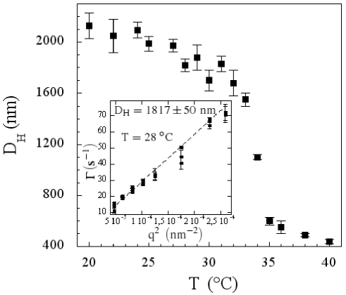
Figure 1: Mean hydrodynamic diameter of the pNIPAm particles as a function of temperature, measured with dynamic light scattering experiments. The polydispersity was found to vary between $5\%$ to $15\%$, depending on the realization. A sharp decrease of the microgel particles size was observed around $\mathrm{T}=32\,^{\circ}$C. Their diameter was multiplied by $5$ from the fully collapsed state at high temperature to the fully swollen state at low temperature, reflecting the small degree of cross-linking. Inset: linear relation between the inverse $\Gamma$ of the correlation function decay time $\tau$ and $q^{2}$, here at $\mathrm{T}=28\,^{\circ}$C. The linear dependency validates that only the diffusion of the particles is probed, and allows us to determine the particles diameter.

2.3 Particle Tracking

The thermal motion of the tracers was recorded using a inverted Leica DM IRB microscope with a $\times 100$ oil immersion objective, coupled to a CMOS camera (Phantom v9). The camera was typically running at $20$ frames per second (fps) in the more concentrated states, and at $500$ fps in the low viscosity suspensions, with a $56\times 56$ $\mu\text{m}^{2}$ field of view. Most of the records were $2\,\cdot 10^{3}$ frames long. Depending on the realization, $10$ to $70$ probe thermal motions could be recorded in the same field of view. For reliable analysis of the Brownian motion, particular attention was brought to record the motion far from the rigid wall imposed by the glass slides.

A home-made image analysis software allowed us to track the bead positions $x(t)$ and $y(t)$ close to the focus plane of the objective. For each probe $i$, the time-averaged mean-squared displacement (MSD), $\langle\Delta r^{2}_{i}(t)\rangle_{t^{\prime}}=\langle[x_{i}(t^{\prime}+t)-x_{i}(t^{\prime})]^{2}+[y_{i}(t^{\prime}+t)-y_{i}(t^{\prime})]^{2}\rangle_{t^{\prime}}$ was calculated, improving the statistical accuracy. When necessary, an ensemble-averaged MSD over all the probes, denoted as $\langle\Delta r^{2}(t)\rangle_{t^{\prime},i}$, could be computed. In the following, $\langle\Delta r^{2}_{i}(t)\rangle_{t^{\prime}}$ will refer to the temporal-averaged MSD for one probe, and $\langle\Delta r^{2}(t)\rangle_{t^{\prime},i}$ to the ensemble and temporal averaged MSD.

In our aging experiments, the recording time was short compared to the aging dynamics, which means that no significative aging was observed during the recording. The system could then be considered to be in a quasi stationary state, at a given aging time, during the recording. The resolution limit of our set-up was tested using a highly concentrated ($95\%$ wt) glycerol solution, and was found to be $15$ nm.

Probability Distribution Functions (PDF) of the tracer displacements (self part of the van Hove correlation function) were also computed for each tracer : $p_{i}\left(\Delta x,t\right)=\langle\delta\left(\Delta x-\Delta x_{i}\left(t\right)\right)\rangle_{t^{\prime}}$, and for the overall sample : $p\left(\Delta x,t\right)=\langle\delta\left(\Delta x-\Delta x_{i}\left(t\right)\right)\rangle_{t^{\prime},i}$, for different lag times $t$, where $\Delta x$ denotes the elementary one-dimensional displacement along the $x$ axis of the field of view and $\delta$ refers to the delta function. In this study, the system is isotropic, and the behaviour was found to be quantitatively the same on both $x$ and $y$ axis.

2.4 Quenching procedure

One important consideration for the investigation of the aging dynamics in glasses is the preparation and reproducibility of the initial glassy state. In colloidal glasses, one has to quench the system from the liquid state by increasing rapidly the volume fraction. In pNIPAM microgel particles suspensions, such a possibility is offered by varying the temperature. This can be achieved rapidly because the swelling / deswelling rate is of the order of the millisecond ³⁸. After a quench, microgel particles which are swollen in a few seconds, generate stresses through the sample, that relax with time.

The microscope objective temperature could be set between $20\,^{\circ}\rm{C}<T<35\,^{\circ}\rm{C}$, using a Bioptechs objective heater coupled with a cooling device. The sample, kept at high temperature on a Peltier plate at $\mathrm{T}=30\,^{\circ}$C, was suddenly placed on the objective, set at a lower temperature. The sample temperature was then controlled through the oil immersion objective in contact. The equilibration of the temperature sample with the immersion oil by thermal diffusion was achieved in a few seconds.

All the quenches described here were performed from our equilibrium ’liquid’ state at $\Phi=\Phi_{0}$, $\mathrm{T}=30\,^{\circ}$C, resulting in a new couple describing the sample ($\Phi$, T). The quench defines the origin of aging times $t_{w}$. At $t_{w}=0$, the volume fraction of the suspension increases in a few milliseconds, and for sufficiently high volume fractions reached after the quench, a glass was formed out of the initial equilibrium liquid. Aging, due to structural relaxations in the deformable soft spheres suspension, was observed.

The relative size of pNIPAm particles to probe particles changes by 20 $\%$, through the quench. As a result, it is not the same in the starting liquid state and in the corresponding glass state. Moreover, the temperature change slightly affects the particles softness. As for the polydispersity, it does not change much between $\mathrm{T}=20\,^{\circ}$ C and $\mathrm{T}=30\,^{\circ}$C. As long as these quantities (relative size of pNIPAm particles to probe particles, particles softness, polydispersity) remain constant during the aging process, after the quench, it will not affect quantitatively our results. It would be an issue to determine quantitatively the phase diagram of such a suspension.

3 Results and discussion

3.1 Aging dynamics in the glass

The aging dynamics of the microgel particles suspension after a quench in temperature, was investigated by looking at the Brownian motion of the tracers. The mean-squared displacement (MSD) of the probes as a function of the lag time, is displayed in Fig. 2, in the reference ’liquid’ state at $\Phi=\Phi_{0}$, $\mathrm{T}=30\,^{\circ}$C, and after quenches of different amplitudes.

In the reference equilibrium state, the MSD of the probes is nearly diffusive, characterized by a nearly linear dependency with the lag time, and no aging could be observed over more than $4$ hours. All the quenches were performed from this ’liquid’ state at $\Phi=\Phi_{0}$, $\mathrm{T}=30\,^{\circ}$C. The suspension viscosity was estimated with the Stokes relation $\eta=4k_{B}Tt/(6\pi R\langle\Delta r^{2}\left(t\right)\rangle_{t^{\prime},i})=6.1\pm 1.1\,\textrm{mPa}\cdot$s, where $R$ is the tracer radius and $k_{B}$ the Boltzmann constant.

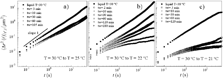
Figure 2: Mean-squared displacement of the tracers ($1\,\mu$m in diameter) as a function of the lag time in the pNIPAM microgel particles suspension, for quenches of different amplitude. Starting from an equilibrium liquid state at $\Phi=\Phi_{0}$, $\mathrm{T}=30\,^{\circ}$C, the sample is quenched down to $\mathrm{T}=25,22$ and $21\,^{\circ}$C, from the left to the right. (a): at $\mathrm{T}=25\,^{\circ}$C, the suspension exhibits an equilibrium visco-elastic behaviour. No aging was observed over more than one hour. The straight line represents the slope 1 corresponding to a purely diffusive behaviour. (b): at $\mathrm{T}=22\,^{\circ}$C, the sample enters a glassy state and slowly ages over several hours. (c): for a deeper quench at $\mathrm{T}=21\,^{\circ}$C, the aging dynamics was found to be faster. (b,c): upon aging, the MSD decreases continuously, and develops a relatively smooth ’plateau’ for large lag times $t$, while it is still diffusive for short lag times. Moreover, the deeper the quench in the glassy state, the faster the glass aging dynamics, i.e. the faster and the deeper the plateau develops.

For a quench from $\mathrm{T}=30\,^{\circ}$C to $\mathrm{T}=25\,^{\circ}$C, the suspension, still at equilibrium, becomes slightly visco-elastic, characterized by a non linear increase of the MSD with the lag time; no aging was observed over more than one hour (Fig. 2(a)). For larger amplitudes quenches – down to $\mathrm{T}=22\,^{\circ}$C and $\mathrm{T}=21\,^{\circ}$C – the suspension was found to fall out-of-equilibrium and to age over hours, indicating that the sample has entered a glassy state, as shown in Fig. 2 (b,c). Upon aging, the MSD decreases continuously, and develops a subdiffusive ’plateau’ at large lag times $t$, while it is still diffusive for short lag times. Moreover, with increasing the quench amplitude, the aging dynamics is faster and the suspension goes in a deeper glass state.

The underlying corresponding picture for the MSD data in the glass state, is the following : the first diffusive regime, at short times, is associated with the motion of the tracer in the cage formed by the surrounding microgel particles. The second regime – smooth plateau becoming deeper upon aging – reflects the elastic response of the cage at the probe length scale. Upon aging, the cage becomes stiffer due to structural relaxations of the soft deformable spheres, and the tracer gets more trapped. Since the pNIPAm particles are soft, the probe can penetrate the shell of the surrounding microgel particles, and the plateau is a ’smooth’ one. In these experiments, the cross over to a diffusive motion of the tracers at larger lag times (cage rearrangement) was not observed, indicating that the tracers remain trapped on the observation time scale.

Here, the glass transition was defined with respect to the out-of-equilibrium regime experienced by the suspension above a certain threshold volume fraction. This is reasonable since no crystal is expected because of the suspension polydispersity. The onset temperature below which the suspension enters a glassy out-of-equilibrium state, was found between $\mathrm{T}=24\,^{\circ}$C and $\mathrm{T}=22\,^{\circ}$C (corresponding to $1.5\,\Phi_{0}<\Phi<1.6\,\Phi_{0}$). Given the relatively small dependence of the microgel particles size as a function of temperature in this range (see Fig. 1), the ’glass transition’ temperature could not be determined with more accuracy.

From the MSD data, a characteristic time $\tau$ associated with the probes diffusion was extracted. This characteristic time was defined as the lag time necessary for a probe to diffuse over a lengthscale $l$, such as $\langle\Delta r^{2}\left(t\right)\rangle_{t^{\prime},i}=l^{2}$. Fig. 3 shows the evolution of the characteristic time $\tau$ with aging time, for two different values of $l^{2}$ – $2.5\,10^{-3}\mu$m² and $5.0\,10^{-3}\mu\mathrm{m}^{2}$ – after a quench from $\mathrm{T}=30\,^{\circ}$C to $\mathrm{T}=22\,^{\circ}$C. On these length scales, typically of the order of one tenth of the probe and pNIPAm particle radius, the characteristic time grows exponentially with aging time by $2$ decades as $\tau\sim\exp(kt_{w})$. Another definition involving $Q\left(l,\tau\right)=\langle e^{-\Delta r_{i}^{2}(\tau)/l^{2}}\rangle_{i,t^{\prime}}=0.6$, where $Q\left(l,\tau\right)$ is a correlation function equivalent to the intermediate scattering function, gave totally similar results ³⁹.

Such an exponential increase of the relaxation time was already observed in other soft glasses and gels, often coupled to a transition to an asymptotic aging regime ($\tau\sim t_{w}$)^{40, 41, 42}. Here the characteristic time we define is not a relaxation time in the usual definition. The asymptotic aging regime might develop at later aging times $t_{w}$, on the considered length scales. Experimentally, no cross over from the exponential growth to the full aging regime could be observed, by changing the quench depth to accelerate the aging process or measuring the characteristic time over $7$ hours.

In these experiments, we probe the dynamical behaviour of the microscopic environment at the scale of the pNIPAm particles, that might be very different from larger scale response. The radius of the probes being of the order of the radius of the pNIPAm particles, there is no scale separation between the probes and the environment constituting elements. We believe that the probes reflect the dynamics of the surrounding pNIPAm colloidal particles, even though the relation between the probes and microgels dynamics is not straightforward and depends on a number of parameters, especially the chemistry of the probes, and the probe size⁴³.

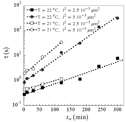
Figure 3: Characteristic times $\tau$ versus aging time $t_{w}$ after quenches at $\mathrm{T}=22\,^{\circ}$C and $\mathrm{T}=21\,^{\circ}$C , recorded over 5 hours. Here, the characteristic time was defined as the lag time needed to reach a certain value $l^{2}$ of the MSD. The characteristic time was found to increase exponentially with aging time, such as $\tau\sim\exp(kt_{w})$.

3.2 Spatially heterogeneous dynamics

3.2.1 The spatial distribution of local Gaussian dynamics behind non Gaussian van Hove functions

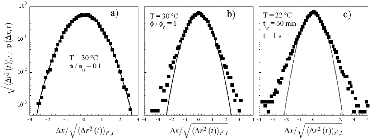
Figure 4: Rescaled Probability Distribution Functions (PDF) of the probes displacement as a function of the rescaled displacement. (a) in the diluted suspension at equilibrium at $\Phi=\Phi_{0}$, $\mathrm{T}=30\,^{\circ}$C, for a lag time $t=0.1$ s. In abscisse, the unity corresponds to $\Delta x=0.6\,R$, where $R$ is the probe radius; (b) in the suspension at $\mathrm{T}=30\,^{\circ}$C, for a lag time $t=0.15$ s. In abscisse, the unity corresponds to $\Delta x=0.38\,R$; (c) in the glass state after a quench from $\mathrm{T}=30^{\circ}$C to $\mathrm{T}=22\,^{\circ}$C, at aging time $t_{w}=60$ min, for a lag time $t=1$ s. In abscisse, the unity corresponds to $\Delta x=0.42\,R$. The black curves are Gaussian fits $Y=\exp\left(-X^{2}\right)/\sqrt{\pi}$. In the diluted suspension, the PDF is a Gaussian, as expected in a purely viscous liquid. In the suspension at $\mathrm{T}=30\,^{\circ}$C, the PDF slightly departs from a Gaussian at large displacements. In the glass state, the PDF exhibits a central Gaussian part for short displacements, and an exponential like decay for large displacements, observed at any lag time and aging time.

We now analyze the probe thermal fluctuations by looking at the Probability Distribution Functions (PDF) of the probes’ displacements (or van Hove functions). Near the glass transition, they have been shown to exhibit non Gaussian shapes, usually assigned to ’dynamic heterogeneity’. Here, we analyze the ensemble-averaged and individual PDF of the tracers.

Figure 4 shows rescaled ensemble-averaged PDF $\sqrt{\langle\Delta r^{2}\left(t\right)\rangle_{t^{\prime},i}}\>\>p(\Delta x,t)$ as a function of the normalized displacement $\Delta x/\sqrt{\langle\Delta r^{2}\left(t\right)\rangle_{t^{\prime},i}}$ in the equilibrium liquid state at different volume fractions, and in the glass state. Experiments performed in the diluted suspension at $\Phi=0.1\,\Phi_{0}$, $\mathrm{T}=30\,^{\circ}$C (dilution factor $10$, purely viscous, viscosity $1.85\pm 0.15$ mPa.s), shows a Gaussian PDF, as expected in a viscous homogeneous fluid (Fig. 4(a)). In the equilibrium reference state at $\Phi=\Phi_{0}$, $\mathrm{T}=30\,^{\circ}$C, the ensemble-averaged PDF were found to be nearly Gaussian at any lag time (Fig. 4(b)), while in the glassy state, they are Gaussian for short displacements, and exhibit an exponential like decay for large displacements, at any lag time allowing for a good statistics ($t<2$ s), and aging time (Fig. 4(c)). As shown here, the shape of the ensemble-averaged PDF changes with increasing volume fraction : it goes from a pure Gaussian at low volume fraction to a PDF with a Gaussian central part for short displacements, and a broad exponential like decay at large displacements, at higher volume fraction. Moreover, the tail of the distribution becomes more pronounced when approaching the glass transition (increasing volume fraction).

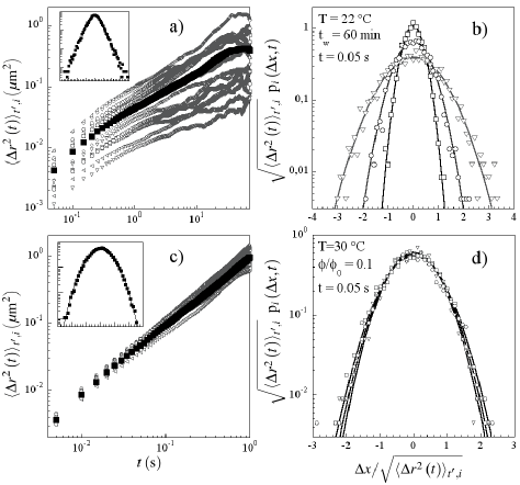
Figure 5: (a): MSD as a function of the lag time for different probes (open symbols) and the ensemble-averaged MSD over the probes (large filled symbols), in the glass state at aging time $t_{w}=60$ min, after a quench from $\mathrm{T}=30\,^{\circ}$C to $\mathrm{T}=22\,^{\circ}$C. A broad spatial distribution of MSD was observed for each $t$. In inset, the corresponding ensemble-averaged PDF is plotted. (b): Individual PDF of the displacements for three probes in the glass state after a quench from $\mathrm{T}=30\,^{\circ}$C to $\mathrm{T}=22\,^{\circ}$C, for a lag time $t=0.05$ s, at aging time $t_{w}=60$ min. For each probe, the individual PDF is a Gaussian with a different width, resulting from a different MSD. (c): the narrow spatial distribution in the diluted liquid state at $\Phi=0.1\,\Phi_{0}$, $\mathrm{T}=30\,^{\circ}$C, with the corresponding Gaussian ensemble-averaged PDF in inset. (d): the individual particles’ displacements distributions are Gaussian, with the same widths.

We now consider the individual motions of the probes through the sample. In the glass state, where the ensemble-averaged PDF were found to depart from a Gaussian, the spatial distribution of the MSD is wide (Fig. 5(a)). The MSD of the individual probes are drastically different from one probe to another, even at shortest lag times where the statistics is the highest. The corresponding individual PDF of the probes’ displacements are Gaussian, $p_{i}(\Delta x,t)\sim\exp{(-(\Delta x(t))^{2}/\Delta_{i})}$, at any lag time allowing for a good statistics ($t<2$ s) and aging times $t_{w}$. Their variance $\Delta_{i}$ were found to be widely distributed through the glass sample (Fig. 5(b)). The resulting ensemble-averaged PDF over all the probes, in the top inset and already shown in Fig. 4(c), exhibits a central Gaussian part, and an exponential like decay at large displacements. By comparison, in the diluted equilibrium liquid state ($\Phi=0.1\,\Phi_{0}$, $\mathrm{T}=30\,^{\circ}$C), the MSD are narrow distributed (Fig. 5(c)). The individual PDF of the probes are Gaussian and similar in width (Fig. 5(d)), and the resulting ensemble-averaged PDF, shown in the bottom inset and in Fig. 4(a), is a Gaussian. In the reference equilibrium state (not shown here, $\Phi=\Phi_{0}$, $\mathrm{T}=30\,^{\circ}$C), the distribution of the individual MSD through the sample is clearly narrower than in the glass state, but wider than in the diluted liquid state. The individual PDF are Gaussian with slightly different widths, and the corresponding PDF slightly departs from a Gaussian at large displacements, as shown in Fig. 4(b).

In the Appendix, we analyze the ensemble-averaged and individual Cumulative Distribution Function (CDF) of the probes’ displacements in the liquid state and in the glass state, in order to clearly identify the shape of the PDF at short and large displacements. Using the CDF to graph the displacements distribution of sample data and try to identify it with respect to known distributions avoids problems of bin size and bin location. We could validate that the ensemble averaged PDF is Gaussian for short displacements, and that its decay at large displacements is well adjusted by an exponential over at least 3 decades in the glass state, while local PDF remain Gaussian (see Appendix).

In our system, the individual distributions of the probes’ displacements were found to be Gaussian, whether at equilibrium or out-of-equilibrium, even though non diffusive, in the considered range of lag times $0.05<t<2$ s, at any volume fraction or age. They are given by $p_{i}(\Delta x,t)\sim\exp{(-(\Delta x(t))^{2}/\Delta_{i})}$, with a variance $\Delta_{i}$ which becomes widely distributed through the sample when approaching the glass transition. The variances $\Delta_{i}$ characterize the local dynamical environment. They can also be considered as a measure of the ’probe mobility’ within the suspension, since the larger the variance $\Delta_{i}$, the more ’mobile’ the probe is.

The scenario behind the non Gaussian van Hove functions is a spatially heterogeneous dynamics of the suspension. At low volume fraction, the spatial distribution of the probes’ mobilities is narrow, revealing an homogeneous suspension, and the ensemble-averaged PDF, $p(\Delta x,t)$, is a Gaussian. With increasing volume fraction, the spatial distribution of the mobilities gets wider, revealing a spatially heterogenous dynamics. A sum of local Gaussians $p_{i}$ of different widths is no longer a Gaussian. As a consequence, the corresponding ensemble-averaged PDF deviates from a Gaussian. The observed non Gaussian tails of the ensemble-averaged $p(\Delta x,t)$ are thus the result of the wide spatial distribution of local dynamical environments $\Delta_{i}$ through the sample.

Spatial heterogeneities already appear below the glass transition in the equilibrium state at $\Phi=\Phi_{0}$, $\mathrm{T}=30\,^{\circ}$C. This suggests that the suspension is already in a ’supercooled’ regime, where a qualitative change in the character of particles motion occurs. The crowding of the suspension is high enough to induce small heterogeneity of dynamics in the sample, but not enough to allow aging, out-of-equilibrium fall, or jamming to occur²⁵.

We now characterize the shape of the distributions $P(\Delta_{i})$ of the individual probes’ mobilities, at equilibrium and out-of-equilibrium. Fig. 6 shows the spatial probability distribution functions of the $\Delta_{i}$, defined such as $\langle\Delta r^{2}_{i}(t)\rangle_{t^{\prime}}=\Delta_{i}(t)$. In the reference liquid state ($\Phi=\Phi_{0}$, $\mathrm{T}=30\,^{\circ}$C) and in the glass state, the distribution is a Gaussian for short diffusion coefficients, and exhibits an exponential decay for large diffusion coefficients (Fig. 6(b,c)). In the diluted liquid state ($\Phi=0.1\Phi_{0}$, $\mathrm{T}=30\,^{\circ}$C), the distribution is centered around a mean diffusion coefficient, and no exponential decay was observed for large diffusion coefficients (Fig. 6(a)). Given a good statistics for the calculation of $\Delta_{i}(t)$, the shape and behaviour of the distributions remains similar for various lag times $t$: the distribution $P(\Delta_{i})$ was found to develop an exponential tail when approaching the glass state. In these experiments, no clear dependence of the distribution shape was found with the aging time.

It is now straightforward to show that, given an exponential tail for the distribution $P(\Delta_{i})$, the resulting ensemble-averaged PDF $p\left(\Delta x,t\right)$ will exhibit an exponential decay at large displacements. We consider the ensemble-averaged PDF as the sum of local Gaussian dynamics $p\left(\Delta x,t\right)=\int\mathrm{d}\Delta_{i}\,P\left(\Delta_{i}\right)\exp{(-(\Delta x(t))^{2}/\Delta_{i})}/\sqrt{\pi\Delta_{i}}$, with a spatial distribution $P\left(\Delta_{i}\right)=\frac{\exp\left(-\Delta_{i}/\Delta_{0}\right)}{\Delta_{0}}$, at large $\Delta_{i}$. The larger the $\Delta_{i}$, the more it contributes to the integral, so we can write : $p\left(\Delta x,t\right)\sim\int\mathrm{d}\Delta_{i}\frac{\exp\left(-\Delta_{i}/\Delta_{0}\right)}{\Delta_{0}}\exp{(-(\Delta x(t))^{2}/\Delta_{i})}/\sqrt{\pi\Delta_{i}}$, which yields, using a method of steepest descent, a leading term for the ensemble averaged PDF at large displacements $p\left(\Delta x,t\right)\sim\exp\left(-2|\Delta x(t)|/\sqrt{\Delta_{0}}\right)$. The exponential decay of the distribution $P(\Delta_{i})$, at large $\Delta_{i}$, results in an exponential decay of the ensemble-averaged PDF.

The exponential decay of $P(\Delta_{i})$ reveals that a small fraction of tracers are intrinsically faster than average. Given that all the individual PDF are Gaussian, the fast particles are responsible for the large displacements in the ensemble-averaged PDF. Here, the exponential decay of the ensemble-averaged PDF is thus the result of the existence of faster mobility zones than average on our observation time scales, rather than jumps experienced by the tracers from time to time. Moreover, in these experiments, no evidence of temporally heterogeneous dynamics was detected on the considered recording times, in the sense that fast regions did not switch from rapid to slow dynamics over time (and vice versa).

We have characterized the statistical distribution of dynamical environments, and show that it can explain the observed exponential tail of the van Hove functions, in the concentrated regimes (supercooled and glass). We analyze quantitatively below how the variance $\sigma^{2}(t)$ of this distribution $P(\Delta_{i})$ evolves when approaching the glass transition, and beyond.

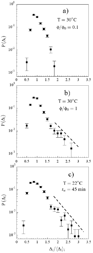
Figure 6: Probability distribution functions of the variances $\Delta_{i}$, defined such as $\langle\Delta r^{2}_{i}(t)\rangle_{t^{\prime}}=\Delta_{i}(t)$. (a) in the diluted liquid state at ($\mathrm{T}=30\,^{\circ}$C, $\Phi=0.1\Phi_{0}$), over $1200$ probes, lag time $t=6\,10^{-3}$ s; (b) in the reference liquid state at ($\mathrm{T}=30\,^{\circ}$C, $\Phi=\Phi_{0}$), over $1150$ probes, lag time $t=3.75\,10^{-2}$ s; (c) in the glass state at $\mathrm{T}=22\,^{\circ}$C and $t_{w}=45$ min, over $1220$ probes, lag time $t=6\,10^{-2}$ s. (b,c): in the reference liquid state and in the glass state, the distribution is a Gaussian for short diffusion coefficients, and exhibits an exponential decay for large diffusion coefficients. No clear dependence of the distribution shape was found with the aging time. (a): in the diluted liquid state, the distribution is centered around a mean diffusion coefficient, and no exponential decay was observed.

3.2.2 Spatial heterogeneities when approaching the glass transition, and beyond

A question that naturally arises now to further characterize the spatial heterogeneities concerns the way they evolve, when approaching and entering the glass state. We now look at the variance $\sigma^{2}(t)$ of the spatial distribution of the $\Delta_{i}(t)=\langle\Delta r^{2}_{i}(t)\rangle_{t^{\prime}}$ through the sample, given by :

$$\frac{\sigma^{2}(\langle\Delta r^{2}_{i}(t)\rangle_{t^{\prime}})}{\langle\Delta r^{2}(t)\rangle^{2}_{t^{\prime},i}}=\frac{\langle(\langle\Delta r^{2}_{i}(t)\rangle_{t^{\prime}}-\langle\Delta r^{2}_{i}(t)\rangle_{t^{\prime},i^{\prime}})^{2}\rangle_{i}}{\langle\Delta r^{2}(t)\rangle^{2}_{t^{\prime},i}}$$

where $\langle\Delta r^{2}_{i}(t)\rangle_{t^{\prime}}$ refers to the temporal-averaged MSD for one probe, and $\langle\Delta r^{2}(t)\rangle_{t^{\prime},i}$ to the ensemble and temporal averaged MSD. This variance gives a measure of the intensity of spatial heterogeneities in the sample. The larger the variance $\sigma^{2}$, the more distributed the variances $\Delta_{i}$ of the individual tracer motion through the sample, and the more the sample is spatially heterogenous.

Figure 7 shows the variance $\sigma^{2}$ of the spatial distribution of the $\langle\Delta r^{2}_{i}(t)\rangle_{t^{\prime}}$ through the sample, as a function of the volume fraction, before and after entering the glass state. Starting from a very diluted liquid state, the variance was found to increase with increasing volume fraction. Given a good statistics for the calculation of $\Delta_{i}(t)$, the variance $\sigma^{2}(t)$ was found to be independent of the lag time $t$, and Figure 7 unchanged. The water represents the reference where no spatial heterogeneities are expected, and sets the sensitivity in our experiments. In thermosensitive suspensions, the value for $\sigma^{2}(t)$ was found to be larger than the experimental sensitivity, which indicates that spatial heterogeneities are present. Figure 7 shows that the suspension dynamics becomes more and more spatially heterogeneous when approaching the glass transition. As seen in section 3.2.1, the dynamics is spatially homogeneous at low concentration ($\Phi/\Phi_{0}=0.1$, $\mathrm{T}=30\,^{\circ}$C), and becomes spatially heterogeneous, already below the glass transition ($\Phi/\Phi_{0}=1$, $\mathrm{T}=30\,^{\circ}$C).

When entering the glass state (above the vertical line), the dynamics remains strongly heterogeneous but also widely distributed. The behaviour of spatial heterogeneities in the glass state during aging is shown in Fig. 8, where we plot the variance $\sigma^{2}$ as a function of a given MSD, $\langle\Delta r^{2}(t)\rangle_{t^{\prime},i}$, at $t=2$ s. We take this MSD as a measure of how deep the suspension is in the glass state after a quench, since this allows us to compare quenches with different final temperatures and different realizations of these quenches, from the same initial equilibrium state. For a given $t$ in the diffusive regime or in the plateau, the variance tends to increase with decreasing amplitude of the $\langle\Delta r^{2}(t)\rangle_{t^{\prime},i}$. This suggests that the deeper the suspension in an arrested state, the more spatially heterogeneous the dynamics.

This work establishes the link between the non Gaussian, exponentially tailed van Hove functions and a spatial distribution of homogeneous dynamic environments in a soft colloidal glass. The intensity of the dynamic heterogeneities is characterized when approaching the glass transition. In aging experiments, reproducibility in the out-of-equilibrium dynamics after a change in the external control parameter, is a major experimental issue. In our experiments, we noticed that taking the aging time $t_{w}$ as a parameter of the ’glass state’ gives qualitatively contradictory results for $\sigma^{2}(t_{w})$, from one realization to the other. However, choosing a given MSD, $\langle\Delta r^{2}(t_{0})\rangle_{t^{\prime},i}$, as a measure of the ’glass state’ leads to the same qualitative behaviours for $\sigma^{2}$ as the suspension goes deeper in the glass state. The dispersion of the data in Fig. 8 certainly comes from the poor statistics consecutive to the use of tracers instead of the microgels themselves. More systematic experiments in the aging regime, improving the statistics, in suspensions with particles of various softness, are currently under investigation.

Dynamic heterogeneities in the aging regime have been investigated in a few studies^{44, 22, 23}, although results in this regime might help to discriminate between theories⁴⁵. Since the particles are almost index matched and impossible to visualize unambiguously on the microscope, the characterization of the shape and size of the regions of homogeneous dynamic environments were beyond the scope of this study, as well as an attempt to question a link between the structure and the dynamic heterogeneities²³. Here, the dynamic heterogeneity is seen as a spatial heterogeneity on the recording time scale, which was chosen to ensure quasi static conditions. Complementary work will investigate the temporal fluctuations of the dynamics and the relation between aging and temporally heterogeneous dynamics.

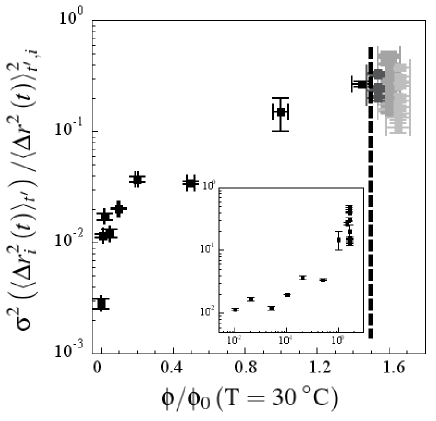
Figure 7: Variance of the spatial distribution of the individual MSD as a function of the relative volume fraction, at equilibrium and in the glass states. The relative volume fraction is defined with respect to the volume fraction $\Phi_{0}$ of the reference equilibrium state at $\mathrm{T}=30\,^{\circ}$C. Given a good statistics for the calculation of $\Delta_{i}(t)$, the variance $\sigma^{2}(t)$ was found to be independent of the lag time. The water represents the reference where no spatial heterogeneities are expected, and sets the sensitivity in our experiments. In thermosensitive suspensions, the value for $\sigma^{2}(t)$ is larger than the sensitivity, which indicates that spatial heterogeneities are present. At equilibrium, the variance increases with increasing volume fraction (roughly exponentially for large volume fractions, as a power law for low volume fractions, see inset), indicating the suspension becomes more and more spatially heterogeneous when approaching the glass transition. In the out-of equilibrium states (above the dashed vertical line), the suspension remains strongly spatially heterogeneous and also widely distributed (the different sets of points correspond to different quenches; within a quench, the different points correspond to different aging times). (inset): corresponding log-log plot.

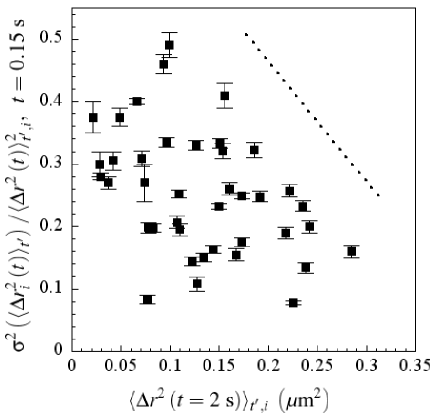
Figure 8: Variance of the distribution of the individual MSD in the glass state, after a quench from $\mathrm{T}=30\,^{\circ}$C to $\mathrm{T}=22\,^{\circ}$C, as a function of a given MSD, at a lag time $t=2$ s. At $\mathrm{T}=30\,^{\circ}$C, the suspension viscosity iss $6.0\pm 0.3$ mPa.s. Although widely distributed, the variance $\sigma^{2}$ tends to decrease with the mean MSD, suggesting that the more the suspension is arrested the more the dynamics is spatially heterogeneous. The dashed line is a guide to the eye.

4 Conclusion

We have investigated the aging dynamics and dynamic heterogeneity of a soft thermosensitive microgels suspension, by looking at the thermal fluctuations of tracers. By varying temperature, the volume fraction could be tuned, and the characteristics of the equilibrium liquid suspension and the out-of-equilibrium glass state during aging, investigated on the same sample. Aging was observed over several hours by quenching the suspension from an initial liquid state at high temperature. With increasing the quench amplitude, the aging dynamics was found to be faster, and the system to enter a deeper glass state. Spatially heterogeneous dynamics was observed to develop below the glass transition, and to persist in the glass state. Individually, the probes always exhibit a Gaussian PDF, whether at equilibrium or in the glass state, revealing a locally homogeneous dynamical environment. With increasing volume fraction, the local dynamical environment was found to change significantly from one probe to another, sign of a spatially heterogeneous dynamics. In the supercooled regime, characterized by a non aging heterogeneous system, and in the glass states, the statistical distribution of these dynamical environments was shown to decay exponentially, indicating that the dynamics is dominated by a small fraction of faster mobility zones than average, rather than jumps experienced by the tracers from time to time, on the experimental timescales. We show that these distributions with exponential tails can explain the observed exponential tails of the van Hove functions. Finally, we analyze the variance of these distributions, as a function of the volume fraction, and as a function of the age in the glass state. It gives a measure of the spatial heterogeneity intensity in our samples. With increasing volume fraction, spatially heterogeneous dynamics was found to amplify. In the glass state, it tends to increase as the suspension gets more arrested.

5 Appendix

5.1 Cumulative Distribution Function

The Cumulative Distribution Function (CDF) $\mathrm{C}\left(x\right)$ of a random variable (e.g. the displacement of a probe particle during a fixed lag time, $\Delta x$) is the probability that this random variable takes a value smaller or equal to $x$ : $\mathrm{C}\left(x\right)=p\left(\Delta x\leq x\right)$. The CDF of a random variable is deduced from its PDF $p$ by integration : $\mathrm{C}\left(x\right)=\int_{-\infty}^{x}\mathrm{d}x^{\prime}p\left(x^{\prime}\right)$. A schematic representation of a typical CDF is presented below :

It monotonically increases from $0$ to $1$, is antisymmetric around the variable median ($0$ in our case) and has a typical width of the order of its standard deviation (square root of the MSD in our case).

Our interest here is to know the detailed shape of the tails of the CDF, for large positive and negative displacements. Since the situation is symmetrical, we focused on positive displacements only. In order to zoom on what happens as $\mathrm{C}\left(x\right)$ reaches $1$, the tail is stretched by computing, for $x>0$, the quantity :

$$y=-\ln\left(2\left(1-\mathrm{C}\left(x\right)\right)\right),$$ (1)

which diverges as $\mathrm{C}\left(x\right)$ goes to $1$ ($x$ to $+\infty$). For the negative tail, we computed $y^{\prime}=\ln\left(2\mathrm{C}\left(x\right)\right)$ and found results in quantitative agreement with those of the positive tail.

Two particular cases were of great interest to us : the case of a Gaussian PDF of the displacements and the case of a PDF of displacements decreasing exponentially for large displacements.
In the case of a Gaussian pdf of the displacements $p\left(\Delta x\right)=\exp\left(-(\Delta x)^{2}/\langle\Delta r^{2}\rangle\right)/\sqrt{\langle\Delta r^{2}\rangle}$, the CDF is given by :

$$\mathrm{C}_{gauss}\left(x\right)=\frac{1+\mathrm{erf}\left(x/\sqrt{\langle\Delta r^{2}\rangle}\right)}{2}.$$ (2)

For large displacements ($x>>\sqrt{\langle\Delta r^{2}\rangle}$), the stretched CDF is given by inserting Eq. 2 in Eq.1 and developping for large $x$ and yields :

$$y_{gauss}=u^{2}+\frac{1}{2}\ln\pi+\ln u+O\left(u^{-2}\right),$$ (3)

where $u=x/\sqrt{\langle\Delta r^{2}\rangle}$. Thus a quadratic variation of $y$ with $x$ at leading order is reminiscent of a Gaussian shape of the PDF of displacements. We fitted variable $y$ in the Gaussian cases with its full expression (Eq. 2 inserted in Eq.1) rather than the large displacement development.

In the case of a PDF with exponential tails, if the PDF of displacements follows the equation $p\left(\Delta x\right)=\exp\left(-|\Delta x|/\lambda\right)/\lambda$ for large $\Delta x$, then The CDF of displacements is given for large $x$ by :

$$\mathrm{C}_{exp}\left(x\right)=1-Be^{-\frac{x}{\lambda}},$$ (4)

where $B$ depends on the detailed shape of the PDF at small displacements. The stretched CDF is then given for large displacements by :

$$y_{exp}=\frac{x}{\lambda}-\ln\left(2B\right).$$ (5)

A linear divergence of the stretched CDF is thus equivalent to an exponential decay of the PDF of displacements.

Finally, if the stretched CDF is fitted by $y=a\,u+b$ ($u=x/\sqrt{\langle\Delta r^{2}\rangle}$), it is easily shown that the PDF of displacements is given by $\frac{a}{2}\exp\left(-b\right)\exp\left(-a\,u\right)$. If the fit is valid on a range $u\in\left[u_{0};u_{1}\right]$, then the PDF decrease exponentially on a number $n$ of decades given by $n=\log_{10}\left(p(u_{0})/p(u_{1})\right)=\left(a\left(u_{1}-u_{0}\right)\right)\log_{10}\left(e\right)$.

Figure 9 shows the individual and ensemble-averaged Cumulative Distribution Functions (CDF) of the probes’ displacements in the low concentration liquid equilibrium state and in the glass state. In the low concentration liquid state, the individual CDF are narrow distributed, indicating a spatially homogeneous suspension. All the CDF in the liquid state, individual and ensemble-averaged, could be adjusted by a parabolic curve indicating a Gaussian behaviour of the corresponding PDF. In the glass state, the individual CDF are widely distributed and still described by a parabolic function, as seen in Figure 9-right. Their ensemble-average results in a linear function, giving evidence of an exponential decay of the associated PDF over 3 decades.

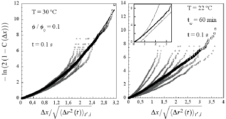
Figure 9: Cumulative distribution functions (CDF) of the probes’ displacements in the liquid equilibrium state (left) and in the glass state (right). The grey symbols represent the individual CDF of the probes while the black symbols are for the ensemble-averaged CDF over the probes. In the liquid state, all the CDF are well described by a Gaussian distribution of displacements and the individual CDF are narrow distributed. In the glassy state, the spreading of individual Gaussian CDF is wide. The inset shows the ensemble-averaged CDF with two fits: a parabolic one at short displacements, and a linear one at large displacements, giving evidence that the displacements distribution is Gaussian-like for small displacement (as expected at first order) and exponential for large displacements.

In the glass phase at $\mathrm{T}=22^{\circ}\mathrm{C}$, we found $a=2.40\pm 0.05$ and $b=-0.40\pm 0.05$, valid over a range $u\in\left[0.7;3.5\right]$. This is equivalent to an exponential decrease of the PDF over $3$ decades.

Acknowledgements

R. C. and B. A. are grateful to F. Van Wijland and C. Gay for very fruitful discussions.

References

- 1 P. N. Pusey and W. van Megen. Phase behavior of concentrated suspensions of nearly hard colloidal spheres. Nature, 320:340–342, March 1986.
- 2 Alfons van Blaaderen and Pierre Wiltzius. Real-space structure of colloidal hard-sphere glasses. Science, 270:1177, November 1995.
- 3 Andrea J. Liu and Sidney R. Nagel. Jamming is not just cool anymore. Nature, 396:21, 1998.
- 4 L. Cipelletti and E. Weeks. Glassy dynamics and dynamical heterogeneities in colloids. arXiv:1009.6089v1[cond-mat.soft], 2010.
- 5 J. Mattson, H. M. Wyss, A. Fernandez-Nieves, K. Miyazaki, Z. Hu, D. R. Reichman, and D. Weitz. Soft colloids make strong glasses. Nature, 462:83, 2009.
- 6 Brian R. Saunders and Brian Vincent. Microgel particules as model colloids : theory, properties and applications. Advances in Colloid and Interface Science, 80:1–25, 1999.
- 7 H. Senff and W. Richtering. Influence of cross-link density on rheological properties of temperature-sensitive microgel suspensions. Colloid Polym. Sci., 278:830–840, February 2000.
- 8 Markus Stieger, Jan Skov Pederson, Peter Lindner, and Walter Richtering. Are thermoresponsive microgels model systems for concentrated colloidal suspensions ? a rheology and small-angle neutron scattering study. Langmuir, 20:7283–7292, June 2004.
- 9 T. Hellweg, C. D. Dewhurst, E. Brückner, K. Kratz, and W. Eimer. Colloidal crystals made of poly(n-isopropylacrylamide) microgel particles. Colloid Polym. Sci., 278:972–978, March 2000.
- 10 L. Andrew Lyon, Justin D. Debord, Saet Byul Debord, Clinton D. Jones, Jonathan G. McGrath, and Michael J. Serpe. Microgel colloidal crystals. Journal of Physical Chemistry B, 108:19099–19108, May 2004.
- 11 A. M. Alsayed, M.F. Islam, J. Zhang, P.J. Collings, and A.G. Yodh. Premelting at defects within bulk colloidal crystals. Science, 309:1207, August 2005.
- 12 Y. Han, N. Y. Ha, A. M. Alsayed, and A. G. Yodh. Melting of two-dimensional tunable-diameter colloidal crystals. Phys. Rev. E, 77:041406, April 2008.
- 13 M. A. Lohr, A. M. Alsayed, B. G. Chen, Z. Zhang, R. D. Kamien, and A. G. Yodh. Helical packings and phase transformations of soft spheres in cylinders. Phys. Rev. E, 81:040401, April 2010.
- 14 Eko H. Purnomo, Dirk van den Ende, Siva A. Vanapalli, and Frieder Mugele. Glass transition and aging in dense suspensions of thermosensitive microgel particles. Phys. Rev. Lett., 101(23):238301, Dec 2008.
- 15 Z. Zhang, N. Xu, D. T. N. Chen, P. Yunker, A. M. Alsayed, K. B. Aptowicz, P. Habdas, A. J. Liu, S. R. Nagel, and A. G. Yodh. Thermal vestige of the zero-temperature jamming transition. Nature, 459:07998, May 2009.
- 16 Dirk van den Ende, Eko H. Purmono, Michel H. G. Duits, Walter Richtering, and Frieder Mugele. Aging in dense suspensions of soft thermoresponsive microgel particles studied with particle-tracking microrheology. Phys. Rev. E, 81:011404, January 2010.
- 17 A. Kasper, E. Bartsch, and H. Sillescu. Self-diffusion in concentrated colloid suspensions studied by digital video microscopy of core-shell tracer particles. Langmuir, page 5004, 1998.
- 18 A. H. Marcus, J. Schofield, and S.A. Rice. Experimental observations of non-gaussian behavior and stringlike cooperative dynamics in concentrated quasi-two-dimensional collidal liquids. Phys. Rev. E, 60:5725, 1999.
- 19 Willem K. Kegel and Alfons van Blaaderen. Direct observation of dynamical heterogeneities in colloidal hard-sphere suspensions. Science, 287:290, January 2000.
- 20 Eirc R. Weeks, John C. Crocker, Andrew C. Levitt, Andrew Schofield, and David A. Weitz. Three-dimentional direct imaging of structural relaxation near the colloidal glass transition. Science, 287:627, January 2000.
- 21 M. Cloitre, R. Borrega, and L. Leibler. Rheological aging and rejuvenation in microgel pastes. Phys. Rev. Lett., 85:4819, 2000.
- 22 J.M. Lynch, G.C. Cianci, and E.R. Weeks. Dynamics and structure of an aging binary colloidal glass. Phys. Rev. E, 78:031410, 2008.
- 23 P. Yunker, Z. Zhang, K. B. Aptowicz, and A. G. Yodh. Phys. Rev. Lett., 103:115701, 2009.
- 24 R. Zorn. Deviation from gaussian behavior in the self-correlation function of the proton motion in polybutadiene. Phys. Rev. B, 55:6249, 1997.
- 25 M.D. Ediger. Spatial heterogeneous dynamics in supercooled liquids. Annual Review of Physical Chemistry, 51:99–128, 2000.
- 26 E. Vidal Russel and N. E. Israeloff. Direct observation of molecular cooperativity near the glass transition. Nature, 2000.
- 27 G. Marty and O. Dauchot. Subdiffusion and cage effect in a sheared granular material. Phys. Rev. Lett., 94(1):015701, Jan 2005.
- 28 A. R. Abate and D. J. Durian. Topological persistence and dynamical heterogeneities near jamming. Phys. Rev. E, 76:021306, 2007.
- 29 B. Doliwa and A. Heuer. Cage effect, local anisotropies, and dynamical heterogeneities at the glass transition: a computer study of hard spheres. Phys. Rev. Lett., 80:4915, 1998.
- 30 S. C. Glotzer. Spatially heterogeneous dynamics in liquids: insights from simulation. Journ. of Non-crystalline Solids, 274:342, 2000.
- 31 D. El Masri, L. Berthier, and L. Cipelletti. Subdiffusion and intermittent dynamic fluctuations in the aging regime of concentrated hard spheres. Phys. Rev. E, 82:031503, 2010.
- 32 Ranko Richert. Heterogeneous dynamics in liquids : fluctuations in space and time. Journal of Physics : Condensed Matter, 14:R703–R738, May 2002.
- 33 Pinaki Chaudhuri, Walter Kob, and Ludovic Berthier. Universal nature of particle displacements close to glass and jamming transitions. Phys. Rev. Lett., 99:060604, august 2007.
- 34 R. Richert. Journ. of Non-crystalline Solids, 172:209, 1994.
- 35 B. Vorselaars, A.V. Lyulin, K. Karatasos, and M.A.J. Michels. Non-gaussian nature of glassy dynammics by cage to cage motion. Phys. Rev. E, 75:011504, 2007.
- 36 D.A. Sessoms, I. Bischofberger, L. Cipelletti, and V. Trappe. Phil. Trans. R. Soc. A, 367:5013 –5032, 2009.
- 37 Bruce J. Berne and Robert Pecora. Dynamic light Scattering With Application to Chemistry, Biology and Physics. Dover Publications, Inc., 2000.
- 38 T. Tanaka and D. J. Filmore. Kinetics of swelling of gels. Journ. of Chem. Phys., 70:1214–1218, 1979.
- 39 Frédéric Lechenault, Olivier Dauchot, Giulio Biroli, and J.P. Bouchaud. Critical scaling and heterogeneous superdiffusion across the jamming/rigidity transition of a granular glass. Europhys. Lett., 83(4):46003, 2008.
- 40 Bérengère Abou, Daniel Bonn, and Jacques Meunier. Aging dynamics in a colloidal glass. Phys. Rev. E, 64(2):021510, July 2001.
- 41 Knaebel A. Bellour, M. and, J. L. Harden, F. Lequeux, and J.-P. Munch. Aging processes and scale dependence in soft glassy colloidal suspensions. Phys. Rev. E, 67(3):031405, March 2003.
- 42 S. Kaloun, R. Skouri, M. Skouri, J. P. Munch, and F. Schosseler. Successive exponential and full aging regimes evidenced by tracer diffusion in a colloidal glass. Phys. Rev. E, 72(1):011403, July 2005.
- 43 T. A. Waigh. Microrheology of complex fluids. Rep. Prog. Phys., 68:685–742, 2005.
- 44 Rachel E. Courtland and Eric R. Weeks. Direct visualization of ageing in colloidal glasses. Journal of Physics : Condensed Matter, 15:S359–S365, January 2003.
- 45 L. Berthier, G. Biroli, J.-P. Bouchaud, and R. L. Jack. Overview of different characterisations of dynamic heterogeneity. arXiv:1009.4765v2[cond-mat.soft], 2010.