Splitting rate matrix as a definition of time reversal in master equation systems

Abstract

Motivated by recent progresses in nonequilibrium Fluctuation Relations, we present a generalized time reversal for stochastic master equation systems with discrete states that is defined as a splitting of the rate matrix into irreversible and reversible parts. An immediate advantage of this definition is that a variety of fluctuation relations can be attributed to different matrix splitting. Additionally, we also find that, the accustomed total entropy production formula and conditions of the detailed balance must be modified appropriately to account for the presence of the reversible part, which was completely ignored in the past a long time.

I Introduction

Fluctuation theorems or fluctuation relations Bochkov77 ; Evans ; Searles ; Gallavotti ; Kurchan ; Lebowitz ; JarzynskiPRL97 ; JarzynskiPRE97 ; Crooks99 ; Crooks00 ; HatanoSasa ; Maes ; SeifertPRL05 ; Speck are a variety of exact equalities about statistics of entropy production or dissipated work that are held even in far from equilibrium regimes. In near-equilibrium region, these relations reduce to the famous fluctuation-dissipation theorems (FDTs) Evans ; Lebowitz ; Callen ; Kubo ; GallavottiPRL96 . The discovery of these fluctuation relations significantly advances our understanding about nonequilibrium physics, and particularly about the second law of thermodynamics of small systems Bustamante .

The fluctuation relations are very relevant with the concept of time reversal Evans ; Searles ; Gallavotti ; Kurchan ; Lebowitz ; JarzynskiPRL97 ; JarzynskiPRE97 ; Crooks99 ; Crooks00 ; HatanoSasa ; Maes ; SeifertPRL05 ; Chernyak ; TCohen . For instance, under the framework of Markovian stochastic systems, previous work has proved that a majority of them can be derived by a ratio of the probability densities of observing a trajectory in a original system and the reversed trajectory in the time-reversed system. Very recently, Chetrite and Gawedzki Chetrite further elaborated this observation and presented a generalized time reversal definition on continuous diffusion processes. Different from conventional definition of time reversal as simply changing time parameter in a stochastic dynamics into minus, they explicitly defined time reversal as a splitting of drift vector into irreversible and reversible parts which possess distinct rules under the transformation of $t$$\to$$-t$. Because of freedom of the splitting, a variety of time reversal and corresponding fluctuation relations are obtained, e.g., the Hatano-Sasa equality HatanoSasa arising from a novel time reversal with nonzero reversible drift. The importance of the generalized time reversal was shown again when we understood the origin of a generalized integral fluctuation relation (GIFR) on general diffusion processes LiuF1 ; LiuF3 .

In addition to the continuous diffusion process, another typical and important Markovian process is master equation with discrete states and continuous time Gardiner . Although the latter is more general than the former in principle, due to their highly formal analogy, many results and evaluations about the fluctuation relations in the diffusion processes could be established correspondingly in the master equation systems Lebowitz ; SeifertPRL05 ; Esposito07 ; Harris ; LiuF2 ; EspositoPRL10 . Nevertheless, whether a similar time reversal definition exists and how to define it are not investigated yet. We must emphasize that it is not trivial as one might think of at first glance. Except for positive transition rates, in these master equation systems there are not quantities such as drift vector and diffusion matrix that have intuitive rules of transformation as time reversed Risken . Somewhat surprisingly, here we will show that an physically relevant answer indeed exists.

The organization of this work is as follows. In sec. II, we briefly review a GIFR in the master equation systems that we found very recently LiuF2 . The reason we use the GIFR rather than other famous fluctuation relations is its generality. Additionally, the necessary of extending the conventional time reversal will be brought forth naturally in deriving the GIFR. In order to interpret an unknown matrix in this relation, in sec. III we present a generalized time reversal in these systems as a splitting of rate matrix into reversal and irreversible parts. The consequences of this new definition will be discussed in sec. IV, which includes reinvestigation of the fluctuation relations from a point of view of the splitting, generalization of total entropy production and conditions of the detailed balance. Section V is the summary.

II Review of the GIFR in the master equation systems

Assume a Markovian process with discrete states and continuous time is described by a master equation LiuF2

$$\frac{dp_{n}(t)}{dt}=\left[{\textbf{H}}(t){\textbf{p}}(t)\right]_{n},$$ (1)

where $n$ is the state index which may be a vector, the $N$-dimensional column vector ${\textbf{p}}(t)$$=$$(p_{1},\cdots,p_{N})^{\rm T}$ is the probability of the system at individual states at time $t$, and the matrix element $({\bf H})_{mn}$=$H_{mn}$$>$0 ($m$$\neq$$n$) is the time dependent or independent rate and $({\textbf{H}})_{nn}$=$-$$\sum_{m\neq n}H_{mn}$. Given a normalized positive column vector ${\textbf{f}}(t)$=$(f_{1},\cdots,f_{N})^{\rm T}$ and a $N$$\times$$N$ matrix A whose elements $({\bf A})_{mn}$$=$$A_{mn}$ ($m\neq n$) satisfy condition $H_{mn}f_{n}$$+$$A_{mn}$$>0$ and $A_{nn}$$=$$-\sum_{m\neq n}A_{mn}$, we found that the inner product ${\textbf{f}}^{\rm T}(t^{\prime}){\textbf{v}}(t^{\prime})$ ($t^{\prime}$$<$$t$) is $t^{\prime}$-invariable if the vector $\textbf{v}(t^{\prime})=(v_{1},\cdots,v_{N})^{\rm T}$ satisfies a perturbed backward equation

$$\frac{dv_{n}(t^{\prime})}{dt^{\prime}}= - ({\textbf{H}}^{\rm T}{\textbf{v}})_{n}$$ (2)

$$- f_{n}^{-1}\left(\partial_{t^{\prime}}{\textbf{f}}-{\textbf{H}}{\textbf{f}}\right)_{n}v_{n}+f_{n}^{-1}[\left({\textbf{A}}\textbf{1}\right)_{n}v_{n}-({\textbf{A}}^{\rm T}{\textbf{v}})_{n}],$$

where the final condition $v_{n}(t)$=$d_{n}$, and $N$-dimension column vector ${\textbf{1}}=(1,\cdots,1)^{\rm T}$. This is easily proved by noticing the time differential property and the transpose property of a matrix. Employing the Feynman-Kac and Girsanov formulas for discrete jump processes LiuF2 , the solution of (2) has a path integral representation given by

$$\sum_{m=1}^{N}f_{m}(0)^{m,0}\langle e^{-{\int_{0}^{t}\cal J}[\textbf{f},\textbf{A}]({\bf x}(\tau))d\tau}d_{{\textbf{x}}(t)}\rangle={\textbf{f}}^{\rm T}(t){\textbf{d}}$$ (3)

and the integrant in the functional is

$${\cal J}[{\bf f,A}] = f_{\textbf{x}(\tau)}^{-1}\left[-\partial_{\tau}\textbf{f}+\textbf{H}\textbf{f}+\textbf{A}\textbf{1}\right]_{{\textbf{x}}(\tau)}+{\cal Q}[f_{\textbf{x}(\tau)}^{-1}\textbf{A}]$$ (4)

with

$${\cal Q}[\textbf{B}] = -B_{{\textbf{x}}(\tau){\textbf{x}}(\tau)}-\ln\left[1+\frac{B_{{\textbf{x}}(\tau^{+}){\textbf{x}}(\tau^{-})}(\tau)}{H_{{\textbf{x}}(\tau^{+}){\textbf{x}}(\tau^{-})}(\tau)}\right]\sum_{i=1}^{k}\delta(\tau-\tau_{i}),$$ (5)

where ${}^{m,0}\langle\rm$ $\rangle$ is the expectation over all trajectories x generated from the system (1) with a fixed state $m$ at initial time 0, $\textbf{x}(\tau)$ is the discrete state of the system at instant time $\tau$, $\textbf{x}(\tau^{-})$ and $\textbf{x}(\tau^{+})$ represent the states just before and after a jump occurring at time $\tau$, respectively, and we have assumed the jumps occur $k$ times for a trajectory. By selecting different ${\bf f}$ and ${\bf A}$, the GIFR (3) may be reduced into different fluctuation relations in the literature LiuF2 .

Although (2) seems complicated, in fact it could be arranged into a concise form:

$$\frac{dq_{\tilde{n}(s)}}{ds}=[\widetilde{\textbf{H}}(s)\textbf{q}(s)]_{\tilde{n}},$$ (6)

where the elements of the probability ${\bf q}(s)$ are

$$q_{\tilde{n}}(s)=[{\bf f}(t)^{\rm T}{\bf d}]^{-1}f_{n}(t^{\prime})v_{n}(t^{\prime})$$ (7)

with $s$=$t$$-$$t^{\prime}$, and the elements of the matrix $\widetilde{\bf H}(s)$ are

$$\widetilde{H}_{{\tilde{n}}{\tilde{m}}}(s)=f_{m}^{-1}(t^{\prime})\left[H_{mn}(t^{\prime})f_{n}(t^{\prime})+A_{mn}(t^{\prime})\right]$$ (8)

for $m$$\neq$$n$ and $\widetilde{H}_{{\tilde{m}}{\tilde{m}}}(s)$$=$$-\sum_{{\tilde{n}}\neq{\tilde{m}}}\widetilde{H}_{{\tilde{n}}{\tilde{m}}}(s)$, and $\tilde{n}$ represents an index whose components are the same or the minus of themselves depending on whether they are even or odd under time reversal $t$$\to$$-t$. Considering that the parameter $s$ is analogous to a reversed time and $\widetilde{H}_{{\tilde{n}}{\tilde{m}}}(s)$$=$${H}_{nm}(t^{\prime})$ as specifically selecting ${\bf A}$ whose elements are the probability flux $[{\bf J}({\bf f})]_{mn}$=$(H_{nm}f_{m}$$-$$H_{mn}f_{n})$, we simply name (6) as generalized time reversal of the original system (1). However, why ${\bf A}$ is almost arbitrary instead of equaling probability flux only was not fully understood previously. Hence, defining the generalized time reversal from a different point of view seems very essential.

III Splitting rate matrix as time reversal

Let us begin with two general matrix identities:

$${[{\textbf{M}}({\bf a.\bf b})]}_{n}-{[{\textbf{M}}{\bf a}]}_{n}b_{n}+a_{n}{[{\textbf{M}}^{\rm T}{\bf b}]}_{n} = [{\textbf{S}}^{\rm T}{\bf b}]_{n}-[{\textbf{S}}{\textbf{1}}]_{n}b_{n},$$ (9)

$${[{\textbf{M}}({\bf a.b})]}_{n}+{[{\textbf{M}}{\bf a}]}_{n}b_{n}-a_{n}{[{\textbf{M}}^{\rm T}{\bf b}]}_{n} = [{\textbf{J}}^{\rm T}{\bf b}]_{n}-[{\textbf{J}}{\bf 1}]_{n}b_{n},$$ (10)

where both ${\bf a}$ and ${\bf b}$ are $N$-dimensional vectors, ${\bf M}$ is $N$$\times$$N$ matrix with $\sum_{m}M_{mn}$$=$$0$, $({\bf a.\bf b})$=$(a_{1}b_{1},\cdots,a_{N}b_{N})^{\rm T}$ represents an array multiplication of the vectors, and the matrixes ${\bf S}$ and ${\bf J}$ are constructed by ${\bf M}$ and ${\bf a}$:

$$({\bf S})_{mn}=M_{nm}a_{m}+M_{mn}a_{n},\hskip 11.38092pt({\bf J})_{mn}=M_{nm}a_{m}-M_{mn}a_{n}.$$ (11)

They are symmetric and antisymmetric, respectively. Proving (9) and (10) is straightforward.

Now we assume that the rate matrix can be splitted into a sum of “reversible” and “irreversible” matrixes, namely ${\bf H}$=${\bf H}^{\rm rev}$+${\bf H}^{\rm irr}$. Particularly, we require $H^{\rm irr}_{mn}$$>$$H^{\rm rev}_{mn}$ ($m$$\neq$$n$), the reason of which will be seen shortly. It is easily to see that $H^{\rm irr}_{mn}$ is always greater than zero for $H_{mn}$$>$0, though the sign of $H^{\rm irr}_{mn}$ is indefinite. We further assume ${\bf H}$ is transformed into ${\bf\widetilde{H}}$=${\bf\widetilde{H}}^{\rm rev}$+${\bf\widetilde{H}}^{\rm irr}$ under time reversal and

$$\widetilde{H}^{\rm irr}_{\tilde{m}\tilde{n}}(s)={H}^{\rm irr}_{mn}(t^{\prime}),\hskip 11.38092pt\widetilde{H}^{\rm rev}_{\tilde{m}\tilde{n}}(s)=-{H}^{\rm rev}_{mn}(t^{\prime}).$$ (12)

Obviously, time-reversed matrix ${\bf\widetilde{H}}$ still possesses rate interpretation. Using these definitions and identities we rewrite the right-hand side of (6) as

$$[\widetilde{\bf H}{\bf q}]_{\tilde{n}} = \frac{1}{{\bf f}(t){\bf d}^{\rm T}}\{[\widetilde{\bf H}^{\rm irr}({\bf f.v})]_{\tilde{n}}+[\widetilde{\bf H}^{\rm rev}({\bf f.v})]_{\tilde{n}}\}$$

$$= \frac{1}{{\bf f}(t){\bf d}^{\rm T}}\{({\textbf{H}}^{\rm T}{\textbf{v}})_{n}-({\textbf{H}}{\textbf{f}})_{n}v_{n}-[(\textbf{J}^{\rm irr}-\textbf{S}^{\rm rev})\textbf{1}]_{n}v_{n}$$

$$\hskip 34.14322pt+[(\textbf{J}^{\rm irr}-\textbf{S}^{\rm rev})^{\rm T}\textbf{v}]_{n}\},$$

where

$$({\textbf{S}}^{\rm rev})_{mn} = H^{\rm rev}_{nm}f_{m}+H^{\rm rev}_{mn}f_{n},$$ (14)

$$({\textbf{J}}^{\rm irr})_{mn} = H^{\rm irr}_{nm}f_{m}-H^{\rm irr}_{mn}f_{n}.$$ (15)

Comparing (III) with (2), we immediately find that

$$[{\bf A(f)}]_{mn} = ({\bf J}^{\rm irr})_{mn}-({\bf S}^{\rm rev})_{mn}$$ (16)

$$= [{\bf J(f)}]_{mn}-2H^{\rm rev}_{nm}f_{m},$$ (17)

(17) implies why the matrix ${\bf A}$ is almost arbitrary: the reversible matrix ${\bf H}^{\rm rev}$ to be determined is responsible for this freedom. In addition, we also notice that the condition of $H_{mn}f_{n}$$+$$A_{mn}$$>$0 mentioned in last section is identical with $H^{\rm irr}_{mn}$$>$$H^{\rm rev}_{mn}$ here.

In practice, we may prior know the matrix ${\bf A}$ or time-reversed rate matrix $\widetilde{\bf H}$. Under these circumstances, the splitting can be constructed conversely as

$$H^{\rm rev}_{nm}=(H_{nm}f_{m}-H_{mn}f_{n}-A_{mn})/2f_{m},$$ (18)

$$H^{\rm irr}_{nm}=(H_{nm}f_{m}+H_{mn}f_{n}+A_{mn})/2f_{m},$$ (19)

or

$$H^{\rm rev}_{mn}(t^{\prime})=[H_{mn}(t^{\prime})-\widetilde{H}_{\tilde{m}\tilde{n}}(s)]/2,$$ (20)

$$H^{\rm irr}_{mn}(t^{\prime})=[H_{mn}(t^{\prime})+\widetilde{H}_{\tilde{m}\tilde{n}}(s)]/2.$$ (21)

Regardless of how a splitting of the rate matrix is achieved, substituting (16) into the integrand (4) we can obtain its new expression given by 

$${\cal J}[{\bf f},\textbf{H}^{\rm irr},\textbf{H}^{\rm rev}] = -\frac{d}{d\tau}\ln f_{{\bf x}(\tau)}(\tau)+{\cal J}[\textbf{1},\textbf{H}^{\rm irr},\textbf{H}^{\rm rev}],$$ (22)

where the second term on the right-hand side is

$$-2\sum_{m\neq{\bf x}(\tau)}H^{\rm rev}_{m{\bf x}(\tau)}-\ln[\frac{H^{\rm irr}_{{\bf x}(\tau^{-}){\bf x}(\tau^{+})}-H^{\rm rev}_{{\bf x}(\tau^{-}){\bf x}(\tau^{+})}}{H^{\rm irr}_{{\bf x}(\tau^{+}){\bf x}(\tau^{-})}+H^{\rm rev}_{{\bf x}(\tau^{+}){\bf x}(\tau^{-})}}]\sum^{k}_{i=1}\delta(\tau-\tau_{i}).$$ (23)

(22) is a consequence of the arbitrariness of ${\bf f}$ in (7), a brief explanation of which is given in Appendix A. Noting (23) also satisfies a fluctuation relation if the initial distribution of the system is uniform. (22) and (23) are the central results of this work.

IV Discussion

Because the physical interpretation of the GIFR (3), its connection with the other fluctuation relations, and its detailed version have been partially investigated LiuF2 , in the remainder we only present several new results obtained from a point of view of the splitting.

IV.1 Total entropy production rate

If ${\bf f}$ is the system’s probability vector ${\bf p}$ and the splitting is prior known from physical consideration, e.g., time reversibility below, (22) is the balance equation of trajectory entropy: the first term on the right-hand side is the change in trajectory system entropy, the second term is the change in trajectory environmental entropy along a specified trajectory, and the left-hand side is the total trajectory entropy. This interpretation has been widely accepted SeifertPRL05 ; Esposito07 ; Harris ; EspositoPRL10 ; GeQian . To our knowledge, however, the expression of the trajectory environmental entropy (23) that involves both even and odd discrete variables is firstly given here. This new formula also reminds us that the total entropy production for the master equation systems with irreversible and reversible rate matrixes is

$$\langle{\cal J}\rangle= - 2\sum_{m\neq n}\sum_{n}H^{\rm rev}_{nm}p_{m}$$ (24)

$$- \sum_{m\neq n}\sum_{n}(H^{\rm irr}_{nm}+H^{\rm rev}_{nm})p_{m}\ln\frac{(H^{\rm irr}_{mn}-H^{\rm rev}_{mn})p_{n}}{(H^{\rm irr}_{nm}+H^{\rm rev}_{nm})p_{m}}\geq 0.$$

The inequality may be proved easily by using ($x$$-1$)$\geq$$\ln x$ or using the Jensen inequality for the GIFR (3). The expression of (24) is significantly distinct from the classical entropy production formula given by Schnakenberg Schnakenberg that involves only even variables.

IV.2 Conditions of the detailed balance

For a time-independent master equation system that has equilibrium state ${\bf p}^{\rm eq}$, we may physically require it invariable under time-reversal, namely, $\widetilde{\bf H}$$=$${\bf H}$. According to (20) and (21) an unique splitting is then

$$H^{\rm rev}_{mn}=(H_{mn}-H_{\tilde{m}\tilde{n}})/2,\hskip 11.38092ptH^{\rm irr}_{mn}=(H_{mn}+H_{\tilde{m}\tilde{n}})/2.$$ (25)

Under this circumstance the irreversible and reversible parts have distinctive properties:

$$H^{\rm rev}_{nm}=-H^{\rm rev}_{{\tilde{n}}{\tilde{m}}},\hskip 11.38092ptH^{\rm irr}_{nm}=H^{\rm irr}_{{\tilde{n}}{\tilde{m}}}.$$ (26)

Obviously, if the discrete master equation system involves only even states, which is exclusively the object investigated in numerous references Gardiner ; Risken ; Oppenheim ; Kampen , the reversible rate matrix must vanish. Because the entropy production is zero when the system is in equilibrium state, according to (24), all terms on its right hand side must vanish. Hence we obtain conditions of detailed balance on the rate matrix and the state which are respectively

$$({\textbf{S}}^{\rm rev})_{mn} = H^{\rm rev}_{nm}p^{\rm eq}_{m}+H^{\rm rev}_{mn}p^{\rm eq}_{n}=0,$$ (27)

$$({\textbf{J}}^{\rm irr})_{mn} = H^{\rm irr}_{nm}p^{\rm eq}_{m}-H^{\rm irr}_{mn}p^{\rm eq}_{n}=0,$$ (28)

$$\sum_{m\neq n}H^{\rm rev}_{mn} = 0.$$ (29)

We must emphasize that, except for the last equation (29) that is from the steady-state requirement and was ignored in previous literature Gardiner ; Risken ; Oppenheim ; Kampen , the former two equations are fully equivalent with the conventional detailed balance condition

$$H_{{\tilde{n}}{\tilde{m}}}p^{\rm eq}_{m}=H_{mn}p^{\rm eq}_{n},$$ (30)

which may be easily checked using (25). We see an unusual side of a time-reversible master equation system with nonvanishing $\textbf{H}^{\rm rev}$: the probability flux $({\bf J})_{mn}$ between two states $m$ and $n$ may be not zero even if the system is in an equilibrium state; both the irreversible and reversible rate matrixes have contributes to the total entropy production. The latter point can be seen more clearly when we rewrite (24) as

$$\langle{\cal J}\rangle= - \sum_{m\neq n}\sum_{n}H^{\rm irr}_{nm}p_{m}\ln\frac{H^{\rm irr}_{mn}p_{n}}{H^{\rm irr}_{nm}p_{m}}$$

$$- \sum_{m\neq n}\sum_{n}H^{\rm rev}_{nm}p_{m}\ln(-\frac{H^{\rm rev}_{mn}p_{n}}{H^{\rm rev}_{nm}p_{m}}).$$

by taking (27)-(29) into account. To our best knowledge, there are very fewer stochastic jump processes with both even and odd variables in the literature. In Appendix B we present a simple mathematical model to exemplify their intriguing features.

IV.3 Jarzynski and Hatano-Sasa equalities

For a time-dependent master equation system, we may select the simplest case with ${\bf A}$=0. Then (18) and (19) become

$${\cal{H}}^{\rm rev}_{nm}=\frac{1}{2f_{m}}(H_{nm}f_{m}-H_{mn}f_{n}),$$ (32)

$${\cal{H}}^{\rm irr}_{nm}=\frac{1}{2f_{m}}(H_{nm}f_{m}+H_{mn}f_{n}).$$ (33)

We used a new notation ${\cal H}$ instead of $H$ to indicate the speciality of this splitting. Under this case, (22) is

$${\cal J}[{\bf f},{\bf A}=0] = -\frac{d}{d\tau}\ln f_{{\bf x}(\tau)}(\tau)+{\cal J}[\textbf{1},{\cal H}^{\rm irr},{\cal H}^{\rm rev}],$$ (34)

and

$${\cal J}[{\bf 1},{\cal H}^{\rm irr},{\cal H}^{\rm rev}]= -\frac{1}{f_{{\bf x}(\tau)}}\sum_{m\neq{{\bf x}}(\tau)}[H_{{\bf x}(\tau)m}f_{m}-H_{m{\bf x}(\tau)}f_{{\bf x}(\tau)}]$$ (35)

$$-\ln\frac{f_{\bf x(\tau^{-})}}{f_{\bf x(\tau^{+})}}\sum^{k}_{i=1}\delta(\tau-\tau_{i}).$$

If one further selects ${\bf f}$ to be the instant equilibrium solution ${\bf p}^{\rm eq}(t)$ or the instant nonequilibrium steady-state solution ${\bf p}^{\rm ss}(t)$ of the master equation if it has, the GIFR is respectively the famous Jarzynski equality about dissipated work JarzynskiPRL97 ; JarzynskiPRE97 or Hatano-Sasa equality about excess entropy HatanoSasa . Noting the first term of the right-hand side of the above equation in both cases vanishes because of the steady-state condition. It is worth pointing out that for the former equality, the detailed balance conditions (27) and (28) imply that such a splitting is trivial because of ${\cal{H}}^{\rm rev}_{nm}(t)$=$H^{\rm rev}_{nm}(t)$ and ${\cal{H}}^{\rm irr}_{nm}(t)$=$H^{\rm irr}_{nm}(t)$, and (35) has other three different but equivalent expressions:

$$\ln\frac{p^{\rm eq}_{{\bf x(\tau^{-})}}}{p^{\rm eq}_{{\bf x(\tau^{+})}}} =\ln\frac{H^{\rm irr}_{{\bf x(\tau^{-})}{\bf x(\tau^{+})}}}{H^{\rm irr}_{{\bf x(\tau^{+})}{\bf x(\tau^{-})}}}=\ln[-\frac{H^{\rm rev}_{{\bf x(\tau^{-})}{\bf x(\tau^{+})}}}{H^{\rm rev}_{{\bf x(\tau^{+})}{\bf x(\tau^{-})}}}]$$ (36)

$$=\ln\frac{H^{\rm irr}_{{\bf x(\tau^{-})}{\bf x(\tau^{+})}}-H^{\rm rev}_{{\bf x(\tau^{-})}{\bf x(\tau^{+})}}}{H^{\rm irr}_{{\bf x(\tau^{+})}{\bf x(\tau^{-})}}+H^{\rm rev}_{{\bf x(\tau^{+})}{\bf x(\tau^{-})}}}.$$

On the other hand, if $\bf A1$$=$$0$ the integrand (4) can be decomposed into

$${\cal J}[{\bf f},{\bf A}]={\cal J}[{\bf f},{\bf 0}]+{\cal Q}[f_{\textbf{x}(\tau)}^{-1}\textbf{A}].$$ (37)

This relationship is very intriguing. In addition that the three terms above satisfy integral fluctuation relation LiuF2 simultaneously, all of them have important physical implications in the nonequilibrium steady-state thermodynamics HatanoSasa ; Speck ; EspositoPRL10 ; GeQian ; Oono . Here we do not repeat previous interpretations but present a simple understanding from a point of view of the splitting. For a nonequilibrium master equation system with ${\bf H}(t)$$=$${\bf H}^{\rm irr}(t)$ and assuming it has unique steady-state as external time-dependent parameter fixed, we have

$${\cal J}[{\bf p},{\bf J(p)}]= - \frac{d}{d\tau}\ln\frac{p_{{\bf x}(\tau)}}{{p}_{{\bf x}(\tau)}^{\rm ss}}+{\cal J}[{\bf p}^{ss},{\bf J(p^{\rm ss})}]$$ (38)

$$= -\frac{d}{d\tau}\ln\frac{p_{{\bf x}(\tau)}}{{p}_{{\bf x}(\tau)}^{\rm ss}}+{\cal J}[{\bf p}^{ss},{\bf 0}]+{\cal Q}[\frac{{\bf J}(p^{\rm ss})}{p_{\bf x(\tau)}^{\rm ss}}]$$ (39)

$$= -\frac{d}{d\tau}\ln p_{{\bf x}(\tau)}+{\cal J}[{\bf 1},{\cal H}^{\rm irr},{\cal H}^{\rm rev}]+{\cal Q}[\frac{{\bf J}(p^{\rm ss})}{p_{\bf x(\tau)}^{\rm ss}}],$$ (40)

where (22), (34), (37) and steady-state condition ${\bf J(p^{\rm ss})1}$=0 are used. (39) implies that trajectory total entropy is the sum of trajectory relative entropy, trajectory excess entropy HatanoSasa , and trajectory housekeeping entropy Speck . Particularly, the sum of the first two terms in (40) that was called as nonadiabatic trajectory entropy EspositoPRL10 is just ${\cal J}[{\bf p},{\cal H}^{\rm irr},{\cal H}^{\rm rev}]$, the ensemble average of which is

$$\langle{\cal J}[{\bf p},{\cal H}^{\rm irr},{\cal H}^{\rm rev}]\rangle= - \sum_{m\neq n}\sum_{n}H_{nm}p_{m}\ln\frac{p^{\rm ss}_{m}p_{n}}{p_{n}^{\rm ss}p_{m}}\geq 0$$ (41)

according to (24). In Ref. GeQian this quantity was also named as free energy dissipation.

V Conclusion

Motivated by the important idea of defining time reversal as a splitting of drift vector in continuous diffusion process, we present the same effort in the master equation system with discrete states. Different from the former, we define the time reversal in this system as a splitting of the rate matrix into irreversible and reversible parts. Even that we find very analogous formulas and results are revealed in these two systems. e.g. (23) corresponding (7.6) in the work of Chetrite and Gawedzki Chetrite or (28) in the work of us LiuF3 . The advantages of introducing this definition are obvious. First, we explain the origin of the matrix $\bf A$ in the GIFR, which was somewhat mysterious to us before starting this work. Second, a variety of fluctuation relations in the master equation systems are unified into various rate matrix splitting. This point was not acknowledged previously. Additionally, the relationships among these fluctuation relations become very clear from this splitting viewpoint, e.g. (39) and (40). Finally, this definition also reminds us the importance of the reversible part of the rate matrix. For instance, the expression of the total entropy production must be modified appropriately. To our knowledge, its existence and implications in the master equation systems were almost completely ignored for a very long time.

This work was supported in part by State Key Laboratory of Software Development Environment SKLSDE-2011ZX-20 and the National Science Foundation of China under Grant No. 11174025.

Appendix A: Derivation of (22) and (23)

For simplicity in notations, we study a specific case of (2) with a final condition is $d_{n}$=1. Under this circumstance the perturbed backward master equation has the time-reversal explanation (6) and

$$q_{\tilde{n}}(s)=f_{n}(t^{\prime})v_{n}(t^{\prime}).$$ (42)

Noting that the initial condition of $q_{\tilde{n}}$ is now $f_{n}(t)$. It is worth emphasizing that we can replace the vector $\bf f$ above by other normalized positive vectors, e.g. $\bf c$=$(1/N,\cdots,1/N)$. Then we have a new relation

$$q_{\tilde{n}}(s)=c_{n}u_{n}(t^{\prime}),$$ (43)

where $u_{n}$ satisfies the same (2) except that $f_{n}$ therein including those in the matrix ${\bf A(f)}$ (16) are substituted by $c_{n}$ and the finial condition becomes $u_{n}(t)$=$f_{n}(t)/c_{n}$. According to (42), (43), and the path integral representation (3), we immediately obtain

$${}^{n,0}\langle e^{-{\int_{0}^{t}\cal J}[\textbf{c},\textbf{A}(\textbf{c})]({\bf x}(\tau))d\tau}\frac{f_{{\textbf{x}}(t)}(t)}{f_{n}(0)}\rangle=^{n,0}\langle e^{-{\int_{0}^{t}\cal J}[\textbf{f},\textbf{A}]({\bf x}(\tau))d\tau}\rangle$$ (44)

Because of ${\cal J}[\textbf{c},\textbf{A}(\textbf{c})]$=${\cal J}[\textbf{1},\textbf{A}(\textbf{1})]$ (22) is proved.

Appendix B: A discrete jump model with both even and odd variables

Figure 1: (a) A discrete jump process with both even (1 and 2) and odd ($\uparrow$ and $\downarrow$) variables, (b) jump process with only even variables (1, 1^′, 2, and 2^′). The letters $r,l,r^{\prime},l^{\prime},u_{1},d_{1},u_{2},d_{2}$ ($>$0) are respective rates.

To show the unusual features of jump processes with both even and odd variables, we develop a simple model; see Fig. (1)(a). Assuming that the variable $i$=1 and $2$ are even and $\uparrow$ and $\downarrow$ are odd, under time reversal ($t$$\rightarrow$$-t$) we have $\widetilde{(i,\uparrow)}=(i,\downarrow)$ and $\widetilde{(i,\downarrow)}=(i,\uparrow)$. Although this model has eight rate parameters, they would not to be independent of each other if we required the model to have a steady-state solution satisfying the detailed balance principle. Using (27)-(29) and performing a simple calculation, we find these rates must obey the following three constraints:

$$lr-l^{\prime}r^{\prime}=0,$$ (45)

$$r-r^{\prime}+d_{1}-u_{1}=0,$$ (46)

$$l-l^{\prime}+d_{2}-u_{2}=0.$$ (47)

The first equation is a consequence of (27) or (28), while the last two equations are from (29). The equilibrium solutions can be easily obtained, which are

$$p^{\rm eq}_{(1,\uparrow)}=p^{\rm eq}_{(1,\downarrow)}=(l+l^{\prime})/2(l+l^{\prime}+r+r^{\prime}),$$ (48)

$$p^{\rm eq}_{(2,\uparrow)}=p^{\rm eq}_{(2,\downarrow)}=(r+r^{\prime})/2(l+l^{\prime}+r+r^{\prime}).$$ (49)

In addition, the total entropy production (IV.2) is

$$\langle{\cal J}\rangle = [d_{1}p_{(1,\uparrow)}-u_{1}p_{(1,\downarrow)}]\ln\frac{p_{(1,\uparrow)}}{p_{(1,\downarrow)}}+[d_{2}p_{2,\uparrow)}-u_{2}p_{(2,\downarrow)}]\ln\frac{p_{(2,\uparrow)}}{p_{(2,\downarrow)}}$$ (50)

$$+ [rp_{(1,\uparrow)}-lp_{(2,\uparrow)}]\ln\frac{(r+r^{\prime})p_{(1,\uparrow)}}{(l+l^{\prime})p_{(2,\uparrow)}}+[r^{\prime}p_{(1,\downarrow)}-l^{\prime}p_{(2,\downarrow)}]\ln\frac{(r+r^{\prime})p_{(1,\downarrow)}}{(l+l^{\prime})p_{(2,\downarrow)}},$$

where $p_{(i,\uparrow)}$ and $p_{(i,\downarrow)}$ are the transient probabilities of the model at distinct states started from an initial distribution. Reader may easily check that, if $p$=$p^{\rm eq}$, the probability currents ${\bf J}$ or the terms before these logarithmic functions above are nonzero.

It would be interesting to compare these results with those obtained in a conventional jump processes with only even variables, e.g. Fig. (1)(b). Its states are respectively marked by the variables 1, 2, 1^′, and 2^′, all of which are even under time reversal. Because of $p^{\rm eq}(i,\uparrow)$=$p^{\rm eq}(i,\downarrow)$ in the model (a), here we additionally require $p^{\rm eq}(i)$=$p^{\rm eq}(i^{\prime})$. Hence, we obtain three constraints on the rates given by

$$d_{1}-u_{1}=0,$$ (51)

$$d_{2}-u_{2}=0,$$ (52)

$$lr^{\prime}-l^{\prime}r=0,$$ (53)

the equilibrium solutions

$$p^{\rm eq}_{1}=p^{\rm eq}_{1^{\prime}}=l/2(r+l),$$ (54)

$$p^{\rm eq}_{2}=p^{\rm eq}_{2^{\prime}}=r/2(r+l),$$ (55)

and the classical total entropy production Schnakenberg

$$\langle{\cal J}\rangle_{c} = (d_{1}p_{1}-u_{1}p_{1^{\prime}})\ln(\frac{d_{1}p_{1}}{u_{1}p_{1^{\prime}}})+(d_{2}p_{2}-u_{2}p_{2^{\prime}})\ln(\frac{d_{2}p_{2}}{u_{2}p_{2^{\prime}}})$$ (56)

$$+ (rp_{1}-lp_{2})\ln(\frac{rp_{1}}{lp_{2}})+(r^{\prime}p_{1^{\prime}}-l^{\prime}p_{2^{\prime}})\ln(\frac{r^{\prime}p_{1^{\prime}}}{l^{\prime}p_{2^{\prime}}}),$$

where $p_{i}$ and $p_{i^{\prime}}$ ($i=$1,2) are the transient probabilities of the model (b) at individual states started from an initial distribution. Obviously, in the model (a) if one did not take the odd variable into account and naively used (56), namely replacing $p_{i}$ and $p_{i^{\prime}}$ therein by $p_{(i,\uparrow)}$ and $p_{(i,\downarrow)}$, respectively, he or she would find that the classical formula would not vanish as the system reaches the equilibrium states (48) and (49). A numerical example to confirm these results is shown in Fig. (2).

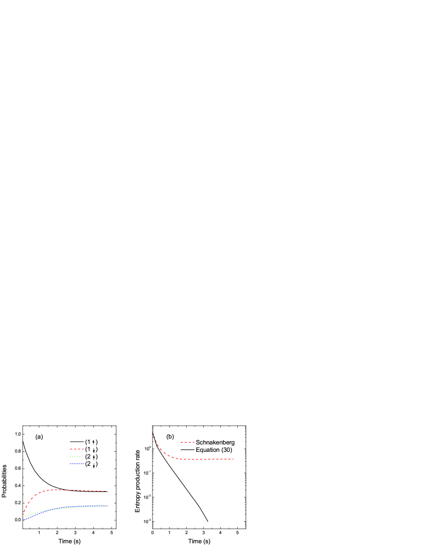
Figure 2: (a) Time evolution of the probabilities at the four states in Fig. (1)(a) and (b) the entropy production rates calculated by the classical Schnakenbergs formula (56) and (IV.2) proposed in this work. We choose $l$=1s^-1, $r$=0.2s^-1, $l_{1}$=0.4s^-1, $r_{1}$=0.5s^-1; $d_{1}$=0.7s^-1; $u_{1}$=0.4s^-1, $d_{2}$=0.2s^-1, and $u_{2}$=0.8s^-1, which satisfy (45)-(47). The initial conditions are $p_{(1,\uparrow)}$=1.0, and the others vanish.

References

References

- (1) Bochkov G N and Kuzovlev Yu E 1977 Sov. Phys. JETP 45 125
- (2) Evans D J Cohen E G D and Morriss G P 1993 Phys. Rev. Lett. 71 2401
- (3) Searles D J and Evans D J 1999 Phys. Rev E 60 159
- (4) Gallavotti G and Cohen E G D 1995 Phys. Rev. Lett. 74 2694
- (5) Kurchan J 1998 J. Phys. A: Math. Gen. 31 3719
- (6) Lebowitz J L and Spohn H 1999 J. Stat. Phys. 95 333
- (7) Jarzynski C 1997 Phys. Rev. Lett. 78 2690
- (8) Jarzynski C 1997 Phys. Rev. E 56 5018
- (9) Crooks G E 1999 Phys. Rev. E 60 2721
- (10) Crooks G E 1999 Phys. Rev. E 61 2361
- (11) Hatano T and Sasa S I 2001 Phys. Rev. Lett. 86 3463
- (12) Maes C 2003 Sem. Poincare 2 29
- (13) Seifert U 2005 Phys. Rev. Lett. 95 040602
- (14) Speck T and Seifert U 2005 J. Phys. A 38 L581
- (15) Callen H B and Welton T A 1951 Phys. Rev. 83 34
- (16) Kubo R 1966 Rep. Prog. Phys. 29 255
- (17) Gallavotti G 1996 Phys. Rev. Lett. 77 4334
- (18) Bustamante C Liphardt J and Ritort F 2005 Phys. Today 58(7) 43
- (19) Chernyak V Cjertkov M and Jarzynski C 2006 J. State. Mech.: Theor. Exp. P08001
- (20) Taniguchi T and Cohen E G D 2008 J. Stat. Phys 130 611
- (21) Chetrite R and Gawedzki K 2008 Commun. Math. Phys. 282 469
- (22) Liu F and Ou-Yang Z C 2009 Phys. Rev. E 79 060107(R)
- (23) Liu F Tong H Ma R and Ou-Yang Z C 2010 J. Phys. A: Math. Theor. 43 495003
- (24) Gardiner C W 1983 Handbook of stochastic methods (Berlin: Springer)
- (25) Esposito M Harbola U and Mukamel S 2007 Phys. Rev. E 76 031132
- (26) Harris R J and Schutz G M 2007 J. Stat. Mech: Theor. Exp. P07020
- (27) Liu F Luo Y P Huang M C and Ou-Yang Z C 2009 J. Phys. A: Math. Gen. 37 332003
- (28) Esposito M and Van den Broeck C 2010 Phys. Rev. Lett 104 090601
- (29) Risken H 1984 The Fokker-Planck equation (Berlin: Springer)
- (30) Ge H and Qian H 2010 Phys. Rev. E 81(051133)
- (31) Schnakenberg J 1976 Rev. Mod. Phys. 48 571
- (32) Oppenheim I Shuler K E and Weiss G H 1977 Stochastic Processes in Chemical Physics-the Master Equation (M.I.T. Press, Cambridge)
- (33) van Kampen N G 1992 Stochastic Processes in physics and chemistry (North Holland, Amsterdam)
- (34) Oono Y and Paniconi M 1998 Prog. Theor. Phys. Suppl. 130 29