Abstract

Four types of photon counters are discussed in terms of information, fidelity, and physical reversibility: conventional photon counter, quantum counter, and their quantum nondemolition (QND) versions. It is shown that when a photon field to be measured is in an arbitrary superposition of vacuum and one-photon states, the quantum counter is the most reversible, the QND version of conventional photon counter provides the most information, and the QND version of quantum counter causes the smallest state change. Our results suggest that the physical reversibility of a counter tends to decrease the amount of information obtained by the counter.

PACS: 03.65.Ta, 03.67.-a, 42.50.Dv
Keywords: quantum measurement, quantum information, photon counter

1 Introduction

When a quantum measurement provides information about a physical system, it inevitably changes the state of the system into another state via non-unitary state reduction. This property is of great interest not only in the foundations of quantum mechanics but also in quantum information processing and communication [1], e.g., in quantum cryptography [2, 3, 4, 5]. However, such a state change by measurement is not necessarily irreversible [6, 7], despite being widely believed to be intrinsically irreversible [8]. A quantum measurement is said to be physically reversible [7, 9] if the pre-measurement state can be recovered from the post-measurement state with a nonzero probability of success by means of a second measurement, referred to as reversing measurement. Recently, physically reversible measurements have been proposed with various systems [10, 11, 12, 13, 14, 15, 16] and discussed in the context of quantum computation [17, 18], and have been experimentally demonstrated using a superconducting phase qubit [19] and a photonic qubit [20]. Therefore, it would be worth discussing the state change by a measurement together with its physical reversibility.

The necessary and sufficient condition for physical reversibility is that the operator $\hat{M}$ describing the state change by the measurement has a bounded left inverse $\hat{M}^{-1}$ [7, 9]. In fact, to recover the pre-measurement state, the reversing measurement is constructed so that it applies $\hat{M}^{-1}$ to the measured system to cancel the effect of $\hat{M}$ when a preferred outcome is obtained. Interestingly, the reversing measurement completely erases the information provided by the first measurement when it successfully recovers the pre-measurement state (see Erratum of Ref. [11]), although a physically reversible measurement actually provides some information about the measured system in contrast to the unitarily reversible measurements [21, 22]. Therefore, a reversing operation based on $\hat{M}^{\dagger}$, instead of $\hat{M}^{-1}$, has been proposed [23], which can approximately recover the pre-measurement state especially with increasing, rather than decreasing, information gain for a weak measurement. Further discussions of information gain by physically reversible measurement can be seen in other studies [24, 25].

In this article, we investigate four types of photon counters to compare them in terms of information gain, state change, and physical reversibility of the photodetection processes. The first counter is a conventional photon counter that operates by absorption of photons, and the second counter is a quantum counter [26, 27] that operates by stimulated emission of photons. The third and fourth counters are the quantum nondemolition (QND) [28] versions of the first and second counters, that is, the QND photon and QND quantum counters, which perform unsharp measurements of photon number without perturbing photon-number states. Among the four counters, quantum counter and its QND version are physically reversible. For each counter, we evaluate the amount of information gain using a decrease in Shannon entropy [25, 23], the degree of state change using fidelity [29], and the degree of physical reversibility using the maximal successful probability of reversing measurement [17], assuming that a photon field to be measured is in an arbitrary superposition of vacuum and one-photon states.

This article is organized as follows: Section 2 reviews a mathematical formulation of quantum measurement and the physical reversibility in quantum measurement. Sections 3, 4, 5, and 6 discuss the conventional photon counter, quantum counter, QND photon counter, and QND quantum counter, respectively, calculating the information gain, fidelity, and physical reversibility in a two-state model. Section 7 summarizes our results, compares the four counters, and discusses an implementation of a QND quantum counter proposed in this article.

2 Quantum Measurement

Here, we briefly review a mathematical formulation of quantum measurement together with its physical reversibility. Let $|\psi\rangle$ be an unknown pre-measurement state of a system to be measured. To obtain information about the state, we perform an indirect measurement using a probe as follows. We first prepare the probe in a state $|i\rangle_{\text{p}}$ and then turn on an interaction between the probe and the system via an interaction Hamiltonian $\hat{H}_{\text{int}}$ during a time interval $\Delta t$. After the interaction, the state of the whole system becomes $\hat{U}_{\text{int}}|\psi\rangle|i\rangle_{\text{p}}$, where $\hat{U}_{\text{int}}=\exp\left(-i\hat{H}_{\text{int}}\Delta t/\hbar\right)$. Finally, we perform a projective measurement on the probe with respect to an orthonormal basis $\{|m\rangle_{\text{p}}\}$. From the outcome $m$, we can indirectly obtain some information about the state. Below we shall show what and how much information we can obtain in the case of photodetection processes.

The measurement yields an outcome $m$ with probability

$$p_{m}=\langle\psi|\hat{M}_{m}^{\dagger}\hat{M}_{m}|\psi\rangle,$$ (1)

where $\hat{M}_{m}={}_{\text{p}}\langle m|\hat{U}_{\text{int}}|i\rangle_{\text{p}}$, and simultaneously changes the state of the system from $|\psi\rangle$ into

$$|\psi_{m}\rangle=\frac{1}{\sqrt{p_{m}}}\hat{M}_{m}\,|\psi\rangle,$$ (2)

depending on the outcome $m$. In other words, a quantum measurement is mathematically described by a set of linear operators $\{\hat{M}_{m}\}$ [30, 1], called measurement operators, that satisfy the completeness condition

$$\sum_{m}\hat{M}_{m}^{\dagger}\hat{M}_{m}=\hat{I},$$ (3)

where $\hat{I}$ is the identity operator. The probability and post-measurement state are then given for each outcome $m$ by Eqs. (1) and (2), respectively. Conversely, for a give set of linear operators $\{\hat{M}_{m}\}$ satisfying the completeness condition (3), an indirect measurement described by $\{\hat{M}_{m}\}$ can always be constructed by choosing the initial state $|i\rangle_{\text{p}}$, the interaction $\hat{U}_{\text{int}}$, and the orthonormal basis $\{|m\rangle_{\text{p}}\}$ of the probe.

Although the measurement changes the state of the system as in Eq. (2), this state change is physically reversible if and only if $\hat{M}_{m}$ has a bounded left inverse [7, 9]. In fact, to undo the state change, consider performing another measurement, called reversing measurement, on the post-measurement state (2). The reversing measurement is described by a set of measurement operators $\{\hat{R}^{(m)}_{\nu}\}$ that satisfy

$$\sum_{\nu}\hat{R}^{(m)\dagger}_{\nu}\hat{R}^{(m)}_{\nu}=\hat{I}$$ (4)

and for a particular $\nu_{0}$,

$$\hat{R}^{(m)}_{\nu_{0}}=\eta_{m}\,\hat{M}_{m}^{-1}$$ (5)

with a complex constant $\eta_{m}$. The index $\nu$ denotes the outcome of the reversing measurement. Therefore, if the reversing measurement yields the particular outcome $\nu_{0}$, it restores the pre-measurement state $|\psi\rangle$ except for an overall phase factor from Eq. (2) as

$$|\psi_{m\nu_{0}}\rangle=\frac{1}{\sqrt{p_{m\nu_{0}}}}\,\hat{R}^{(m)}_{\nu_{0}}\,|\psi_{m}\rangle\propto|\psi\rangle,$$ (6)

where

$$p_{m\nu_{0}}=\langle\psi_{m}|\hat{R}^{(m)\dagger}_{\nu_{0}}\hat{R}^{(m)}_{\nu_{0}}|\psi_{m}\rangle=\frac{|\eta_{m}|^{2}}{p_{m}}$$ (7)

is the probability for the second outcome $\nu_{0}$ given the first outcome $m$, and thus is the successful probability of the reversing measurement. Since the completeness condition (4) requires $\langle\psi^{\prime}|\hat{R}^{(m)\dagger}_{\nu_{0}}\hat{R}^{(m)}_{\nu_{0}}|\psi^{\prime}\rangle\leq 1$ for any state $|\psi^{\prime}\rangle$, the upper bound for $|\eta_{m}|^{2}$ becomes [17]

$$|\eta_{m}|^{2}\leq\inf_{|\psi^{\prime}\rangle}\,\langle\psi^{\prime}|\hat{M}_{m}^{\dagger}\hat{M}_{m}|\psi^{\prime}\rangle\equiv b_{m},$$ (8)

which does not depend on the pre-measurement state $|\psi\rangle$. The upper bound $b_{m}$ is called the background of $\hat{M}_{m}$, implying that the measurement $\{\hat{M}_{m}\}$ yields the outcome $m$ with a probability not less than $b_{m}$ for any state. Combining Eqs. (7) and (8), we find that if the pre-measurement state is $|\psi\rangle$ and the first outcome is $m$, the maximal successful probability of the reversing measurement is given by

$$R\bigl{(}m,|\psi\rangle\bigr{)}\equiv\max_{\eta_{m}}\,p_{m\nu_{0}}=\frac{b_{m}}{p_{m}}.$$ (9)

That is, we can, in principle, recover the unknown pre-measurement state $|\psi\rangle$ from the post-measurement state $|\psi_{m}\rangle$ with the probability (9), even though it would be difficult to experimentally implement the reversing measurement $\{\hat{R}^{(m)}_{\nu}\}$ with $|\eta_{m}|^{2}=b_{m}$ as an indirect measurement.

3 Photon Counter

A photon counter usually detects photons one by one from a photon field. This means that the photon counter detects at most one photon during a short time interval. When detecting one photon (“one-count” process), the counter annihilates the detected photon from the photon field. Even in the case when no photon is detected (“no-count” process), the counter changes the state of the photon field owing to the obtained information that no photon was detected during the time interval. A physical model of the photon counter is described in accordance with the indirect measurement in Sec. 2. In this case, the probe is a two-level atom having a ground state $|g\rangle_{\text{p}}$ and an excited state $|e\rangle_{\text{p}}$ with a raising operator $\hat{\sigma}_{+}=|e\rangle_{\text{p}\,\text{p}}\langle g|$ and a lowering operator $\hat{\sigma}_{-}=|g\rangle_{\text{p}\,\text{p}}\langle e|$. The initial state of the atom is the ground state $|g\rangle_{\text{p}}$, and the interaction Hamiltonian between the atom and the photon field is the Jaynes-Cummings Hamiltonian

$$\hat{H}_{\text{int}}=\hbar g\left(\hat{a}\hat{\sigma}_{+}+\hat{a}^{\dagger}\hat{\sigma}_{-}\right),$$ (10)

where $g$ is a coupling constant, and $\hat{a}^{\dagger}$ and $\hat{a}$ are the creation and annihilation operators of the photon. The projective measurement on the atom is with respect to the basis $\{|g\rangle_{\text{p}},|e\rangle_{\text{p}}\}$. As a result of the measurement, if the atom is found to be in the excited state $|e\rangle_{\text{p}}$, we recognize that the one-count process has occurred with the absorption of a photon. On the other hand, if the atom is found to be still in the ground state $|g\rangle_{\text{p}}$, we recognize that the no-count process has occurred with detecting no photon.

In terms of the measurement operator in Sec. 2, the one- and no-count processes are described by [31, 32, 7],

$$\hat{M}_{1}=\gamma\hat{a},\qquad\hat{M}_{0}\simeq\hat{I}-\frac{\gamma^{2}}{2}\hat{a}^{\dagger}\hat{a},$$ (11)

respectively, where $\gamma=g\Delta t$ is a constant that is assumed to be so small that we can ignore the fourth and higher order terms in $\gamma$. In fact, the annihilation operator in $\hat{M}_{1}$ annihilates a photon from the photon field through the state reduction (2) in the one-count process. Moreover, combined with $\hat{M}_{1}$, the measurement operator $\hat{M}_{0}$ for the no-count process satisfies the completeness condition (3), i.e.,

$$\sum_{m=0,1}\hat{M}_{m}^{\dagger}\hat{M}_{m}\simeq\hat{I}$$ (12)

up to the order of $\gamma^{3}$. This means that we can regard the one-count and no-count processes as a mutually exclusive and exhaustive set of events in the measurement.

3.1 General Model

To evaluate the amount of information provided by the photon counter, we assume that the pre-measurement state of the photon field is known to be one of the predefined pure states $\{|\psi(a)\rangle\}$ with equal probability, $p(a)=1/N$, where $a=1,\ldots,N$, although the pre-measurement state is unknown. Because in quantum measurement the pre-measurement state is usually an arbitrary unknown state, the set $\{|\psi(a)\rangle\}$ is essentially an infinite set ($N\to\infty$) to cover the Hilbert space of the photon field. Each state can be expanded by the eigenstates $\{|n\rangle\}$ of the photon-number operator $\hat{a}^{\dagger}\hat{a}$ as

$$|\psi(a)\rangle=\sum_{n}c_{n}(a)\,|n\rangle$$ (13)

with $n=0,1,2,\ldots$, and the coefficients $\{c_{n}(a)\}$ that obey the normalization condition $\sum_{n}\left|c_{n}(a)\right|^{2}=1$. Our lack of information about the photon field can be quantified by the Shannon entropy associated with the probability distribution $\{p(a)\}$ as

$$H_{0}=-\sum_{a}p(a)\log_{2}p(a)=\log_{2}N.$$ (14)

Next, we perform a measurement by the photon counter (11) to obtain a piece of information about the photon field. According to Eq. (1), if the pre-measurement state is $|\psi(a)\rangle$, the one-count process occurs with probability

$$p^{\text{PC}}(1|a)=\langle\psi(a)|\hat{M}_{1}^{\dagger}\hat{M}_{1}|\psi(a)\rangle=\gamma^{2}n_{1}(a),$$ (15)

where

$$n_{1}(a)\equiv\sum_{n}n\left|c_{n}(a)\right|^{2}.$$ (16)

Since the probability for $|\psi(a)\rangle$ is $p(a)=1/N$, the total probability for the one-count process is given by

$$p^{\text{PC}}(1)=\sum_{a}p^{\text{PC}}(1|a)\,p(a)=\frac{1}{N}\sum_{a}\gamma^{2}n_{1}(a)=\gamma^{2}\overline{n_{1}},$$ (17)

where the overline denotes the average over $a$,

$$\overline{f}\equiv\frac{1}{N}\sum_{a}f(a).$$ (18)

On the contrary, given that the photon counter detects one photon, we can find the probability for the pre-measurement state $|\psi(a)\rangle$ as

$$p^{\text{PC}}(a|1)=\frac{p^{\text{PC}}(1|a)\,p(a)}{p^{\text{PC}}(1)}=\frac{n_{1}(a)}{N\overline{n_{1}}}$$ (19)

from Bayes’ rule. Using this probability distribution, our lack of information after the one-count process is evaluated by the Shannon entropy as follows:

$$H^{\text{PC}}(1)=-\sum_{a}p^{\text{PC}}(a|1)\log_{2}p^{\text{PC}}(a|1)=\log_{2}N-\frac{\overline{n_{1}\log_{2}n_{1}}-\overline{n_{1}}\log_{2}\overline{n_{1}}}{\overline{n_{1}}}.$$ (20)

The information gain by the one-count process is then defined by the decrease in Shannon entropy as

$$I^{\text{PC}}(1)=H_{0}-H^{\text{PC}}(1)=\frac{\overline{n_{1}\log_{2}n_{1}}-\overline{n_{1}}\log_{2}\overline{n_{1}}}{\overline{n_{1}}},$$ (21)

which does not depend on $\gamma$ (i.e., on the coupling constant $g$ between the photon counter and the photon field). That is, this information gain is a measure of how much our knowledge about the pre-measurement state increases when we revise the probability distribution from $p(a)=1/N$ to $p^{\text{PC}}(a|1)$ according to the outcome. Note that it results from a single measurement outcome [25, 23] without averaging all the outcomes, and that it indicates the state of the pre-measurement rather than a value of some observable. Similar to the one-count process, we obtain the total probability for the no-count process which is given as $p^{\text{PC}}(0)\simeq 1-\gamma^{2}\overline{n_{1}}$; this information gain by the no-count process is $I^{\text{PC}}(0)\simeq 0$ up to the order of $\gamma^{3}$. Therefore, averaging over the outcomes $m=0,1$, we find that the mean information gain by the measurement is given by

$$I^{\text{PC}}=\sum_{m}p^{\text{PC}}(m)\,I^{\text{PC}}(m)\simeq\gamma^{2}\left(\,\overline{n_{1}\log_{2}n_{1}}-\overline{n_{1}}\log_{2}\overline{n_{1}}\,\right),$$ (22)

which is identical to the mutual information [1] of the random variables $\{a\}$ and $\{m\}$:

$$I^{\text{PC}}=\sum_{m,a}p^{\text{PC}}(a|m)\,p^{\text{PC}}(m)\,\log_{2}\frac{p^{\text{PC}}(a|m)}{p(a)}.$$ (23)

Unfortunately, the measurement changes the state of the photon field. The state change can be evaluated by the fidelity [29, 1] between the pre-measurement and post-measurement states. According to Eq. (2), when the pre-measurement state is $|\psi(a)\rangle$, the post-measurement state after the one-count process is

$$|\psi(1,a)\rangle^{\text{PC}}=\frac{1}{\sqrt{p^{\text{PC}}(1|a)}}\,\hat{M}_{1}|\psi(a)\rangle=\frac{1}{\sqrt{n_{1}(a)}}\sum_{n}\sqrt{n+1}\,c_{n+1}(a)\,|n\rangle,$$ (24)

whose fidelity to $|\psi(a)\rangle$ is

$$F^{\text{PC}}(1,a)=\bigl{|}\langle\psi(a)|\psi(1,a)\rangle^{\text{PC}}\bigr{|}=\frac{1}{\sqrt{n_{1}(a)}}\left|\sum_{n}\sqrt{n+1}\,c_{n}^{\ast}(a)\,c_{n+1}(a)\right|.$$ (25)

Since the index $a$ is unknown, we average over $a$ with the probability (19) to obtain the fidelity after the one-count process as

$$F^{\text{PC}}(1)=\sum_{a}p^{\text{PC}}(a|1)\,F^{\text{PC}}(1,a)=\overline{\frac{\sqrt{n_{1}}}{\overline{n_{1}}}\left|\sum_{n}\sqrt{n+1}\,c_{n}^{\ast}\,c_{n+1}\right|}.$$ (26)

On the other hand, the fidelity after the no-count process is $F^{\text{PC}}(0)\simeq 1$ up to the order of $\gamma^{3}$. The mean fidelity after the measurement is thus given by

$$F^{\text{PC}}=\sum_{m}p^{\text{PC}}(m)\,F^{\text{PC}}(m)\simeq 1-\gamma^{2}\overline{n_{1}}+\gamma^{2}\overline{\sqrt{n_{1}}\left|\sum_{n}\sqrt{n+1}\,c_{n}^{\ast}\,c_{n+1}\right|}.$$ (27)

We can, however, undo this state change of the photon field if the measurement is physically reversible as described in Sec. 2. The physical reversibility can be evaluated by the maximal successful probability (9) of the reversing measurement. If the pre-measurement state is $|\psi(a)\rangle$ and the outcome is the one-count process, it becomes

$$R^{\text{PC}}(1,a)=\frac{b^{\text{PC}}(1)}{p^{\text{PC}}(1|a)}=\frac{n_{1\text{i}}}{n_{1}(a)},$$ (28)

where $b^{\text{PC}}(1)$ is the background of $\hat{M}_{1}$ defined in Eq. (8), namely,

$$b^{\text{PC}}(1)=\inf_{a^{\prime}}p^{\text{PC}}(1|a^{\prime})=\gamma^{2}\inf_{a^{\prime}}n_{1}(a^{\prime})\equiv\gamma^{2}n_{1\text{i}}.$$ (29)

Averaging over $a$ with the probability (19), we find the reversibility of the one-count process as

$$R^{\text{PC}}(1)=\sum_{a}p^{\text{PC}}(a|1)\,R^{\text{PC}}(1,a)=\frac{n_{1\text{i}}}{\,\overline{n_{1}}\,}.$$ (30)

Similarly, using the background of $\hat{M}_{0}$,

$$b^{\text{PC}}(0)=\inf_{a^{\prime}}p^{\text{PC}}(0|a^{\prime})\simeq 1-\gamma^{2}\sup_{a^{\prime}}n_{1}(a^{\prime})\equiv 1-\gamma^{2}n_{1\text{s}},$$ (31)

the reversibility of the no-count process is found to be

$$R^{\text{PC}}(0,a)=\frac{b^{\text{PC}}(0)}{p^{\text{PC}}(0|a)}\simeq\frac{1-\gamma^{2}n_{1\text{s}}}{1-\gamma^{2}n_{1}(a)}$$ (32)

if the pre-measurement state is $|\psi(a)\rangle$, and is

$$R^{\text{PC}}(0)=\sum_{a}p^{\text{PC}}(a|0)\,R^{\text{PC}}(0,a)\simeq\frac{1-\gamma^{2}n_{1\text{s}}}{1-\gamma^{2}\overline{n_{1}}}$$ (33)

if averaged over $a$. The mean reversibility of the measurement thus becomes

$$R^{\text{PC}}=\sum_{m}p^{\text{PC}}(m)\,R^{\text{PC}}(m)\simeq 1-\gamma^{2}\left(n_{1\text{s}}-n_{1\text{i}}\right).$$ (34)

It is easy to check from Eqs. (19), (28), and (30) that

$$R^{\text{PC}}=\sum_{m}\inf_{a^{\prime}}p^{\text{PC}}(m|a^{\prime}).$$ (35)

That is, the quantity (34) is identical to the degree of physical reversibility of measurement discussed by Koashi and Ueda [17].

3.2 Two-state Model

As an example, we consider a situation where the photon field is in an arbitrary superposition of the states $|0\rangle$ and $|1\rangle$. That is, the set of predefined states $\{|\psi(a)\rangle\}$ consists of all possible states of the form

$$|\psi(a)\rangle=\cos\frac{\theta}{2}\,|0\rangle+e^{i\phi}\sin\frac{\theta}{2}\,|1\rangle,$$ (36)

where $0\leq\theta\leq\pi$ and $0\leq\phi<2\pi$. The index $a$ now represents the two continuous angles $(\theta,\phi)$. Therefore, the probability $p(a)=1/N$ is replaced with a probability density $p(a)=1/4\pi$ using the volume element $\sin\theta d\theta d\phi$ and the summation over $a$ is replaced with an integral over $(\theta,\phi)$, namely,

$$\frac{1}{N}\sum_{a}\quad\longrightarrow\quad\frac{1}{4\pi}\int^{2\pi}_{0}d\phi\,\int^{\pi}_{0}d\theta\sin\theta.$$ (37)

If the pre-measurement state is $|\psi(a)\rangle$, the probability (15) for the one-count process is

$$p^{\text{PC}}(1|a)=\gamma^{2}\sin^{2}\frac{\theta}{2},$$ (38)

since for the state $|\psi(a)\rangle$ in Eq. (36) we have

$$n_{1}(a)=\sum_{n=0,1}n\left|c_{n}(a)\right|^{2}=\left|c_{1}(a)\right|^{2}=\sin^{2}\frac{\theta}{2}.$$ (39)

The total probability (17) for the one-count process then becomes

$$p^{\text{PC}}(1)=\frac{1}{2}\gamma^{2},$$ (40)

because of

$$\overline{n_{1}}=\frac{1}{N}\sum_{a}n_{1}(a)=\frac{1}{4\pi}\int^{2\pi}_{0}d\phi\,\int^{\pi}_{0}d\theta\sin\theta\times\sin^{2}\frac{\theta}{2}=\frac{1}{2}.$$ (41)

On the contrary, given the one-count process, the probability density (19) for the pre-measurement state $|\psi(a)\rangle$ is

$$p^{\text{PC}}(a|1)=\frac{1}{2\pi}\sin^{2}\frac{\theta}{2},$$ (42)

while the corresponding probability density for the no-count process is

$$p^{\text{PC}}(a|0)\simeq\frac{1}{4\pi}\left[1-\gamma^{2}\left(\sin^{2}\frac{\theta}{2}-\frac{1}{2}\right)\right].$$ (43)

These probability densities are the content of information provided by the photon counter (11). Figure 1 shows these densities as functions of $\theta$ when $\gamma=0.3$. Although all the states were equally probable before the measurement, as shown by the dotted line, the one-count process increases the possibility of $|1\rangle$ and completely excludes the possibility of $|0\rangle$, as shown by the line $p^{\text{PC}}(a|1)$. On the contrary, the no-count process decreases the possibility of $|1\rangle$ and increases the possibility of $|0\rangle$, as shown by the line $p^{\text{PC}}(a|0)$, but so slightly that $I^{\text{PC}}(0)\simeq 0$.

Figure 1: Probability density for the pre-measurement state $|\psi(a)\rangle$ conditioned by the one-count process $p^{\text{PC}}(a|1)$ and that conditioned by the no-count process $p^{\text{PC}}(a|0)$ as functions of $\theta$ when $\gamma=0.3$. The dotted line indicates the initial probability density $p(a)=1/4\pi$.

Calculating

$$\overline{n_{1}\log_{2}n_{1}} =\frac{1}{N}\sum_{a}n_{1}(a)\log_{2}n_{1}(a)$$

$$=\frac{1}{4\pi}\int^{2\pi}_{0}d\phi\,\int^{\pi}_{0}d\theta\sin\theta\times\sin^{2}\frac{\theta}{2}\log_{2}\sin^{2}\frac{\theta}{2}=-\frac{1}{4\ln 2}$$ (44)

with $\log_{2}x=\ln x/\ln 2$, we obtain the information gain (21) by the one-count process as

$$I^{\text{PC}}(1)=1-\frac{1}{2\ln 2}\simeq 0.279$$ (45)

and the mean information gain (22) by the measurement as

$$I^{\text{PC}}\simeq\left(\frac{1}{2}-\frac{1}{4\ln 2}\right)\gamma^{2}\simeq 0.139\gamma^{2}.$$ (46)

Furthermore, the fidelity (26) after the one-count process becomes

$$F^{\text{PC}}(1) =\overline{\frac{\sqrt{n_{1}}}{\overline{n_{1}}}\bigl{|}\,c_{0}^{\ast}\,c_{1}\bigr{|}}=\frac{1}{N}\sum_{a}\frac{\sqrt{n_{1}(a)}}{\overline{n_{1}}}\bigl{|}\,c_{0}^{\ast}(a)\,c_{1}(a)\bigr{|}$$

$$=\frac{1}{4\pi}\int^{2\pi}_{0}d\phi\,\int^{\pi}_{0}d\theta\sin\theta\times 2\sin^{2}\frac{\theta}{2}\cos\frac{\theta}{2}=\frac{8}{15}$$ (47)

and the mean fidelity (27) after the measurement becomes

$$F^{\text{PC}}\simeq 1-\frac{7}{30}\gamma^{2}.$$ (48)

Since $n_{1\text{i}}=\inf_{a^{\prime}}n_{1}(a^{\prime})=0$ with $|\psi(a^{\prime})\rangle=|0\rangle$ and $n_{1\text{s}}=\sup_{a^{\prime}}n_{1}(a^{\prime})=1$ with $|\psi(a^{\prime})\rangle=|1\rangle$, the reversibilities (30) and (33) of the one-count and no-count processes are given by

$$R^{\text{PC}}(1) =0,$$ (49)

$$R^{\text{PC}}(0) \simeq 1-\frac{1}{2}\gamma^{2},$$ (50)

respectively. The mean reversibility (34) of the measurement is thus

$$R^{\text{PC}}\simeq 1-\gamma^{2}.$$ (51)

From Eq. (49), we can see that the one-count process of the photon counter (11) is not physically reversible. This means that we can never recover the pre-measurement state from the post-measurement state unless we know the pre-measurement state. The irreversibility originates from the fact that the photon counter does not respond to the vacuum state [6], namely, $p^{\text{PC}}(1|a)=0$ for $|\psi(a)\rangle=|0\rangle$.

4 Quantum Counter

A quantum counter is a photon counter that operates by stimulated emission, rather than by absorption, of photons. It was proposed to detect infrared photons [26] or to measure antinormally ordered correlation functions [27, 33], and was discussed to show reversibility in quantum measurement [6]. A physical model of the quantum counter is the indirect measurement with the two-level atom and the Jaynes-Cummings Hamiltonian (10) as in the photon counter in Sec. 3. However, in this case, the atom is first prepared in the excited state $|e\rangle_{\text{p}}$. After the interaction and the projective measurement, if the atom is found to be in the ground state $|g\rangle_{\text{p}}$, we recognize that the one-count process has occurred with the emission of a photon. On the other hand, if the atom is found to be still in the excited state $|e\rangle_{\text{p}}$, we recognize that the no-count process has occurred with detecting no photon.

The action of the quantum counter is described by the measurement operators for one-count and no-count processes [6, 7]

$$\hat{L}_{1}=\gamma\hat{a}^{\dagger},\qquad\hat{L}_{0}\simeq\hat{I}-\frac{\gamma^{2}}{2}\hat{a}\hat{a}^{\dagger}.$$ (52)

As seen from $\hat{L}_{1}$, the quantum counter creates a new photon in the photon field by stimulated or spontaneous emission in the one-count process through the state reduction (2) as opposed to the conventional photon counter (11). Similar to $\hat{M}_{1}$ and $\hat{M}_{0}$, the measurement operators $\hat{L}_{1}$ and $\hat{L}_{0}$ also satisfy the completeness condition (3) as

$$\sum_{m=0,1}\hat{L}_{m}^{\dagger}\hat{L}_{m}\simeq\hat{I},$$ (53)

up to the order of $\gamma^{3}$.

4.1 General Model

The amount of information provided by the quantum counter (52) can be evaluated using the predefined states $\{|\psi(a)\rangle\}$ as in Sec. 3. If the pre-measurement state is $|\psi(a)\rangle$, the probability for the one-count process is

$$p^{\text{QC}}(1|a)=\langle\psi(a)|\hat{L}_{1}^{\dagger}\hat{L}_{1}|\psi(a)\rangle=\gamma^{2}\left[n_{1}(a)+1\right]$$ (54)

from Eq. (1). Note that the one-count process occurs even when the photon field is in the vacuum state, $|\psi(a)\rangle=|0\rangle$, owing to spontaneous emission, unlike the conventional photon counter [see Eq. (15)]. In this sense, the quantum counter is sensitive not only to photons but also to the vacuum state. The total probability for the one-count process is then

$$p^{\text{QC}}(1)=\sum_{a}p^{\text{QC}}(1|a)\,p(a)=\gamma^{2}\left(\overline{n_{1}}+1\right).$$ (55)

On the contrary, given the one-count process, the probability for the pre-measurement state $|\psi(a)\rangle$ is

$$p^{\text{QC}}(a|1)=\frac{p^{\text{QC}}(1|a)\,p(a)}{p^{\text{QC}}(1)}=\frac{n_{1}(a)+1}{N\left(\overline{n_{1}}+1\right)}.$$ (56)

Calculating the Shannon entropy $H^{\text{QC}}(1)$ associated with this probability distribution, we find the information gain by the one-count process as

$$I^{\text{QC}}(1)=H_{0}-H^{\text{QC}}(1)=\frac{\overline{(n_{1}+1)\log_{2}(n_{1}+1)}-(\overline{n_{1}}+1)\log_{2}(\overline{n_{1}}+1)}{\overline{n_{1}}+1}.$$ (57)

This quantifies the increase in our knowledge about the pre-measurement state when we revise the probability distribution from $p(a)=1/N$ to $p^{\text{QC}}(a|1)$ according to the outcome. Similarly, the total probability for the no-count process is $p^{\text{QC}}(0)\simeq 1-\gamma^{2}\left(\overline{n_{1}}+1\right)$ and the information gain by the no-count process is $I^{\text{QC}}(0)\simeq 0$ up to the order of $\gamma^{3}$. The mean information gain by the measurement then becomes

$$I^{\text{QC}} =\sum_{m}p^{\text{QC}}(m)\,I^{\text{QC}}(m)$$

$$\simeq\gamma^{2}\left[\,\overline{(n_{1}+1)\log_{2}(n_{1}+1)}-(\overline{n_{1}}+1)\log_{2}(\overline{n_{1}}+1)\,\right].$$ (58)

On the other hand, the state change owing to the measurement can be evaluated by fidelity. When the pre-measurement state is $|\psi(a)\rangle$, the post-measurement state after the one-count process is, from Eq. (2),

$$|\psi(1,a)\rangle^{\text{QC}}=\frac{1}{\sqrt{p^{\text{QC}}(1|a)}}\,\hat{L}_{1}|\psi(a)\rangle=\frac{1}{\sqrt{n_{1}(a)+1}}\sum_{n}\sqrt{n}\,c_{n-1}(a)\,|n\rangle,$$ (59)

whose fidelity to $|\psi(a)\rangle$ is

$$F^{\text{QC}}(1,a)=\bigl{|}\langle\psi(a)|\psi(1,a)\rangle^{\text{QC}}\bigr{|}=\frac{1}{\sqrt{n_{1}(a)+1}}\left|\sum_{n}\sqrt{n}\,c_{n}^{\ast}(a)\,c_{n-1}(a)\right|.$$ (60)

Averaging over $a$ with the probability (56), we find that the fidelity after the one-count process is

$$F^{\text{QC}}(1)=\sum_{a}p^{\text{QC}}(a|1)\,F^{\text{QC}}(1,a)=\overline{\frac{\sqrt{n_{1}+1}}{\overline{n_{1}}+1}\left|\sum_{n}\sqrt{n}\,c_{n}^{\ast}\,c_{n-1}\right|}.$$ (61)

Since the fidelity after the no-count process is $F^{\text{QC}}(0)\simeq 1$ up to the order of $\gamma^{3}$, the mean fidelity after the measurement is given by

$$F^{\text{QC}}=\sum_{m}p^{\text{QC}}(m)\,F^{\text{QC}}(m)\simeq 1-\gamma^{2}(\overline{n_{1}}+1)+\gamma^{2}\overline{\sqrt{n_{1}+1}\left|\sum_{n}\sqrt{n}\,c_{n}^{\ast}\,c_{n-1}\right|}.$$ (62)

Moreover, the reversibility of the measurement can be evaluated by the maximal successful probability (9) of its reversing measurement. If the pre-measurement state is $|\psi(a)\rangle$, the reversibilities of the one-count and no-count processes are

$$R^{\text{QC}}(1,a) =\frac{b^{\text{QC}}(1)}{p^{\text{QC}}(1|a)}=\frac{n_{1\text{i}}+1}{n_{1}(a)+1},$$ (63)

$$R^{\text{QC}}(0,a) =\frac{b^{\text{QC}}(0)}{p^{\text{QC}}(0|a)}\simeq\frac{1-\gamma^{2}\left(n_{1\text{s}}+1\right)}{1-\gamma^{2}\left[n_{1}(a)+1\right]},$$ (64)

respectively, from the background $b^{\text{QC}}(m)=\inf_{a^{\prime}}p^{\text{QC}}(m|a^{\prime})$ in Eq. (8). Averaging over $a$ with the probability (56), we obtain

$$R^{\text{QC}}(1) =\sum_{a}p^{\text{QC}}(a|1)\,R^{\text{QC}}(1,a)=\frac{n_{1\text{i}}+1}{\overline{n_{1}}+1},$$ (65)

$$R^{\text{QC}}(0) =\sum_{a}p^{\text{QC}}(a|0)\,R^{\text{QC}}(0,a)\simeq\frac{1-\gamma^{2}\left(n_{1\text{s}}+1\right)}{1-\gamma^{2}\left(\overline{n_{1}}+1\right)}.$$ (66)

The mean reversibility of the measurement is thus given by

$$R^{\text{QC}}=\sum_{m}p^{\text{QC}}(m)\,R^{\text{QC}}(m)\simeq 1-\gamma^{2}\left(n_{1\text{s}}-n_{1\text{i}}\right).$$ (67)

4.2 Two-state Model

As an example, we consider the situation discussed in Sec. 3. If the pre-measurement state is $|\psi(a)\rangle$, the probability (54) for the one-count process is

$$p^{\text{QC}}(1|a)=\gamma^{2}\left(\sin^{2}\frac{\theta}{2}+1\right)$$ (68)

from Eq. (39). The total probability (55) for the one-count process is then

$$p^{\text{QC}}(1)=\frac{3}{2}\gamma^{2}$$ (69)

owing to Eq. (41). On the contrary, given the one-count process, the probability density (56) for the pre-measurement state $|\psi(a)\rangle$ is

$$p^{\text{QC}}(a|1)=\frac{1}{6\pi}\left(\sin^{2}\frac{\theta}{2}+1\right).$$ (70)

Similarly, given the no-count process, the probability density for $|\psi(a)\rangle$ is

$$p^{\text{QC}}(a|0)\simeq\frac{1}{4\pi}\left[1-\gamma^{2}\left(\sin^{2}\frac{\theta}{2}-\frac{1}{2}\right)\right].$$ (71)

Figure 2 shows these probability densities as functions of $\theta$ when $\gamma=0.3$. The one-count process of the quantum counter (52) deforms the probability density to a smoother slope than that done by the conventional photon counter (11), not excluding the possibility of $|0\rangle$ owing to the sensitivity to the vacuum state.

Figure 2: Probability density for the pre-measurement state $|\psi(a)\rangle$ conditioned by the one-count process $p^{\text{QC}}(a|1)$ and that conditioned by the no-count process $p^{\text{QC}}(a|0)$ as functions of $\theta$ when $\gamma=0.3$. The dotted line indicates the initial probability density $p(a)=1/4\pi$.

Using

$$\overline{(n_{1}+1)\log_{2}(n_{1}+1)}=2-\frac{3}{4\ln 2},$$ (72)

we find the information gain (57) by the one-count process as

$$I^{\text{QC}}(1)=\frac{7}{3}-\frac{1}{2\ln 2}-\log_{2}3\simeq 0.0270$$ (73)

and the mean information gain (58) by the measurement as

$$I^{\text{QC}}\simeq\left(\frac{7}{2}-\frac{3}{4\ln 2}-\frac{3}{2}\log_{2}3\right)\gamma^{2}\simeq 0.0405\gamma^{2}.$$ (74)

Moreover, the fidelity (61) after the one-count process is

$$F^{\text{QC}}(1)=\overline{\frac{\sqrt{n_{1}+1}}{\overline{n_{1}}+1}\bigl{|}\,c_{1}^{\ast}\,c_{0}\bigr{|}}=\frac{1}{3}\,\mathrm{B}\!\left(\frac{3}{4},\frac{3}{2}\right)\simeq 0.320$$ (75)

and the mean fidelity (62) after the measurement is

$$F^{\text{QC}}\simeq 1-\frac{3}{2}\left[1-\frac{1}{3}\,\mathrm{B}\!\left(\frac{3}{4},\frac{3}{2}\right)\right]\gamma^{2}\simeq 1-1.02\gamma^{2},$$ (76)

where $\mathrm{B}(p,q)$ is the beta function. The reversibilities (65) and (66) of the one-count and no-count processes are then

$$R^{\text{QC}}(1) =\frac{2}{3},$$ (77)

$$R^{\text{QC}}(0) \simeq 1-\frac{1}{2}\gamma^{2},$$ (78)

respectively. Equation (77) shows that the one-count process of the quantum counter (52) is physically reversible. That is, we can, in principle, recover the pre-measurement state from the post-measurement state with probability $2/3$ on average, even though it would be difficult to experimentally implement the reversing measurement of the quantum counter. The reversibility is because of the sensitivity to the vacuum state, namely, $p^{\text{QC}}(1|a)>0$ even for $|\psi(a)\rangle=|0\rangle$. The mean reversibility (67) of the measurement is then given by

$$R^{\text{QC}}\simeq 1-\gamma^{2}.$$ (79)

5 QND Photon Counter

Next, we consider a QND version of the conventional photon counter. Its measurement operators for one-count and no-count processes are given by [34, 7]

$$\hat{N}_{1}=\gamma\hat{a}^{\dagger}\hat{a},\qquad\hat{N}_{0}\simeq\hat{I}-\frac{\gamma^{2}}{2}\left(\hat{a}^{\dagger}\hat{a}\right)^{2},$$ (80)

respectively. This counter neither absorbs nor emits a photon in both the one-count and no-count processes through the state reduction (2), thereby not perturbing the photon-number states $\{|n\rangle\}$ to perform an unsharp QND measurement of photon number. The measurement operators $\hat{N}_{1}$ and $\hat{N}_{0}$ also satisfy the completeness condition (3), namely,

$$\sum_{m=0,1}\hat{N}_{m}^{\dagger}\hat{N}_{m}\simeq\hat{I},$$ (81)

up to the order of $\gamma^{3}$.

A physical model of the QND photon counter is an indirect measurement described in Sec. 2. In this case, the probe is an atom having two degenerate states $|a\rangle_{\text{p}}$ and $|b\rangle_{\text{p}}$ with a transition operator $\hat{\sigma}=|b\rangle_{\text{p}\,\text{p}}\langle a|$. The initial state of the atom is the state $|a\rangle_{\text{p}}$, and the interaction Hamiltonian between the atom and the photon field is

$$\hat{H}_{\text{int}}=\hbar g\hat{a}^{\dagger}\hat{a}\left(\hat{\sigma}+\hat{\sigma}^{\dagger}\right).$$ (82)

Performing the projective measurement with respect to the basis $\{|a\rangle_{\text{p}},|b\rangle_{\text{p}}\}$, we recognize that the one-count process has occurred if the atom is found to be in the state $|b\rangle_{\text{p}}$ or that the no-count process has occurred if the atom is found to be still in the state $|a\rangle_{\text{p}}$.

5.1 General Model

To evaluate the amount of information provided by the QND photon counter (80), we consider the set of predefined states $\{|\psi(a)\rangle\}$ described in Sec. 3. If the pre-measurement state is $|\psi(a)\rangle$, the probability for the one-count process is

$$p^{\text{QPC}}(1|a)=\langle\psi(a)|\hat{N}_{1}^{\dagger}\hat{N}_{1}|\psi(a)\rangle=\gamma^{2}n_{2}(a)$$ (83)

owing to Eq. (1), where

$$n_{2}(a)\equiv\sum_{n}n^{2}\left|c_{n}(a)\right|^{2}.$$ (84)

Then, the total probability for the one-count process is given by

$$p^{\text{QPC}}(1)=\sum_{a}p^{\text{QPC}}(1|a)\,p(a)=\gamma^{2}\overline{n_{2}}.$$ (85)

On the contrary, given the one-count process, the probability for the pre-measurement state $|\psi(a)\rangle$ is

$$p^{\text{QPC}}(a|1)=\frac{p^{\text{QPC}}(1|a)\,p(a)}{p^{\text{QPC}}(1)}=\frac{n_{2}(a)}{N\overline{n_{2}}}.$$ (86)

Therefore, we obtain the information gain by the one-count process as

$$I^{\text{QPC}}(1)=H_{0}-H^{\text{QPC}}(1)=\frac{\overline{n_{2}\log_{2}n_{2}}-\overline{n_{2}}\log_{2}\overline{n_{2}}}{\overline{n_{2}}},$$ (87)

where $H^{\text{QPC}}(1)$ is the Shannon entropy associated with the probability distribution (86). This means that our knowledge about the pre-measurement state increases by $I^{\text{QPC}}(1)$ when we revise the probability distribution from $p(a)=1/N$ to $p^{\text{QPC}}(a|1)$ according to the outcome. On the other hand, the total probability for the no-count process is $p^{\text{QPC}}(0)\simeq 1-\gamma^{2}\overline{n_{2}}$ and the information gain by the no-count process is $I^{\text{QPC}}(0)\simeq 0$ up to the order of $\gamma^{3}$. The mean information gain by the measurement thus becomes

$$I^{\text{QPC}}=\sum_{m}p^{\text{QPC}}(m)\,I^{\text{QPC}}(m)\simeq\gamma^{2}\left(\,\overline{n_{2}\log_{2}n_{2}}-\overline{n_{2}}\log_{2}\overline{n_{2}}\,\right).$$ (88)

Then, we evaluate the state change owing to the measurement using fidelity. When the pre-measurement state is $|\psi(a)\rangle$, the post-measurement state after the one-count process is, from Eq. (2),

$$|\psi(1,a)\rangle^{\text{QPC}}=\frac{1}{\sqrt{p^{\text{QPC}}(1|a)}}\,\hat{N}_{1}|\psi(a)\rangle=\frac{1}{\sqrt{n_{2}(a)}}\sum_{n}n\,c_{n}(a)\,|n\rangle,$$ (89)

with the fidelity to $|\psi(a)\rangle$ being

$$F^{\text{QPC}}(1,a)=\bigl{|}\langle\psi(a)|\psi(1,a)\rangle^{\text{QPC}}\bigr{|}=\frac{n_{1}(a)}{\sqrt{n_{2}(a)}}.$$ (90)

Averaging over $a$ with the probability (86), we obtain the fidelity after the one-count process as

$$F^{\text{QPC}}(1)=\sum_{a}p^{\text{QPC}}(a|1)\,F^{\text{QPC}}(1,a)=\frac{\overline{\sqrt{n_{2}}\,n_{1}}}{\overline{n_{2}}}.$$ (91)

Since the fidelity after the no-count process is $F^{\text{QPC}}(0)\simeq 1$, the mean fidelity after the measurement becomes

$$F^{\text{QPC}}=\sum_{m}p^{\text{QPC}}(m)\,F^{\text{QPC}}(m)\simeq 1-\gamma^{2}\overline{n_{2}}+\gamma^{2}\overline{\sqrt{n_{2}}\,n_{1}}.$$ (92)

Furthermore, we evaluate the reversibility of the measurement using the maximal successful probability (9) of its reversing measurement. From the background in Eq. (8), $b^{\text{QPC}}(m)=\inf_{a^{\prime}}p^{\text{QPC}}(m|a^{\prime})$, with $n_{2\text{i}}=\inf_{a^{\prime}}n_{2}(a^{\prime})$ and $n_{2\text{s}}=\sup_{a^{\prime}}n_{2}(a^{\prime})$, the reversibilities of the one-count and no-count processes are

$$R^{\text{QPC}}(1,a) =\frac{b^{\text{QPC}}(1)}{p^{\text{QPC}}(1|a)}=\frac{n_{2\text{i}}}{n_{2}(a)},$$ (93)

$$R^{\text{QPC}}(0,a) =\frac{b^{\text{QPC}}(0)}{p^{\text{QPC}}(0|a)}\simeq\frac{1-\gamma^{2}n_{2\text{s}}}{1-\gamma^{2}n_{2}(a)},$$ (94)

respectively, if the pre-measurement state is $|\psi(a)\rangle$. Therefore, they become

$$R^{\text{QPC}}(1) =\sum_{a}p^{\text{QPC}}(a|1)\,R^{\text{QPC}}(1,a)=\frac{n_{2\text{i}}}{\,\overline{n_{2}}\,},$$ (95)

$$R^{\text{QPC}}(0) =\sum_{a}p^{\text{QPC}}(a|0)\,R^{\text{QPC}}(0,a)\simeq\frac{1-\gamma^{2}n_{2\text{s}}}{1-\gamma^{2}\overline{n_{2}}},$$ (96)

respectively, if averaged over $a$ with probability (86). The mean reversibility of the measurement is then given by

$$R^{\text{QPC}}=\sum_{m}p^{\text{QPC}}(m)\,R^{\text{QPC}}(m)\simeq 1-\gamma^{2}\left(n_{2\text{s}}-n_{2\text{i}}\right).$$ (97)

5.2 Two-state Model

We again consider the situation discussed in Sec. 3 as an example. If the pre-measurement state is $|\psi(a)\rangle$, the probability (83) for the one-count process is

$$p^{\text{QPC}}(1|a)=\gamma^{2}\sin^{2}\frac{\theta}{2},$$ (98)

since using Eq. (36) we have

$$n_{2}(a)=\sum_{n=0,1}n^{2}\left|c_{n}(a)\right|^{2}=\sin^{2}\frac{\theta}{2}.$$ (99)

Note that $n_{2}(a)=n_{1}(a)$ in this two-state model since $n^{2}=n$ for $n=0,1$. Therefore, from Eq. (41), we obtain

$$\overline{n_{2}}=\frac{1}{2}.$$ (100)

The total probability (85) for the one-count process is thus given by

$$p^{\text{QPC}}(1)=\frac{1}{2}\gamma^{2}.$$ (101)

On the contrary, given the one-count process, the probability density (86) for $|\psi(a)\rangle$ is

$$p^{\text{QPC}}(a|1)=\frac{1}{2\pi}\sin^{2}\frac{\theta}{2},$$ (102)

and the corresponding probability density for the no-count process is

$$p^{\text{QPC}}(a|0)\simeq\frac{1}{4\pi}\left[1-\gamma^{2}\left(\sin^{2}\frac{\theta}{2}-\frac{1}{2}\right)\right].$$ (103)

These probability densities are shown in Fig. 3, which is the same form as Fig. 1 owing to $n_{2}(a)=n_{1}(a)$ in this two-state model.

Figure 3: Probability density for the pre-measurement state $|\psi(a)\rangle$ conditioned by the one-count process $p^{\text{QPC}}(a|1)$ and that conditioned by the no-count process $p^{\text{QPC}}(a|0)$ as functions of $\theta$ when $\gamma=0.3$. The dotted line indicates the initial probability density $p(a)=1/4\pi$.

Since we have

$$\overline{n_{2}\log_{2}n_{2}}=-\frac{1}{4\ln 2}$$ (104)

as in Eq. (44), the information gain (87) by the one-count process becomes

$$I^{\text{QPC}}(1)=1-\frac{1}{2\ln 2}\simeq 0.279$$ (105)

and the mean information gain (88) by the measurement becomes

$$I^{\text{QPC}}\simeq\left(\frac{1}{2}-\frac{1}{4\ln 2}\right)\gamma^{2}\simeq 0.139\gamma^{2}.$$ (106)

On the other hand, the fidelity (91) after the one-count process is

$$F^{\text{QPC}}(1)=\frac{\overline{\sqrt{n_{2}}\,n_{1}}}{\overline{n_{2}}}=\frac{4}{5}$$ (107)

and the mean fidelity (92) after the measurement is

$$F^{\text{QPC}}\simeq 1-\frac{1}{10}\gamma^{2}.$$ (108)

In addition, since we have $n_{2\text{i}}=\inf_{a^{\prime}}n_{2}(a^{\prime})=0$ with $|\psi(a^{\prime})\rangle=|0\rangle$ and $n_{2\text{s}}=\sup_{a^{\prime}}n_{2}(a^{\prime})=1$ with $|\psi(a^{\prime})\rangle=|1\rangle$, the reversibilities (95) and (96) of the one-count and no-count processes are given by

$$R^{\text{QPC}}(1) =0,$$ (109)

$$R^{\text{QPC}}(0) \simeq 1-\frac{1}{2}\gamma^{2},$$ (110)

respectively. As shown in Eq. (109), the one-count process of the QND photon counter (80) is not physically reversible. We cannot recover the pre-measurement state from the post-measurement state as in the case of the conventional photon counter (11). Note that the QND photon counter is not sensitive to the vacuum state owing to $p^{\text{QPC}}(1|a)=0$ for $|\psi(a)\rangle=|0\rangle$. The mean reversibility (97) of the measurement is thus

$$R^{\text{QPC}}\simeq 1-\gamma^{2}.$$ (111)

6 QND Quantum Counter

In this section, we propose a novel type of photon counter, that is, a QND version of the quantum counter, whose measurement operators for one-count and no-count processes are written as

$$\hat{Q}_{1}=\gamma\hat{a}\hat{a}^{\dagger},\qquad\hat{Q}_{0}\simeq\hat{I}-\frac{\gamma^{2}}{2}\left(\hat{a}\hat{a}^{\dagger}\right)^{2},$$ (112)

respectively. This counter performs a reversible QND measurement of photon number because it is sensitive not only to photons but also to the vacuum state without perturbing the photon-number states $\{|n\rangle\}$. Of course, the measurement operators $\hat{Q}_{1}$ and $\hat{Q}_{0}$ satisfy the completeness condition (3),

$$\sum_{m=0,1}\hat{Q}_{m}^{\dagger}\hat{Q}_{m}\simeq\hat{I},$$ (113)

up to the order of $\gamma^{3}$. A physical model of the QND quantum counter is similar to that of the QND photon counter described in Sec. 5. The only difference is that the interaction Hamiltonian between the atom and the photon field is now

$$\hat{H}_{\text{int}}=\hbar g\hat{a}\hat{a}^{\dagger}\left(\hat{\sigma}+\hat{\sigma}^{\dagger}\right),$$ (114)

instead of Eq. (82).

6.1 General Model

The amount of information provided by the QND quantum counter (112) is evaluated using the set of predefined states $\{|\psi(a)\rangle\}$ as in Sec. 3. If the pre-measurement state is $|\psi(a)\rangle$, the probability for the one-count process is

$$p^{\text{QQC}}(1|a)=\langle\psi(a)|\hat{Q}_{1}^{\dagger}\hat{Q}_{1}|\psi(a)\rangle=\gamma^{2}n_{3}(a),$$ (115)

according to Eq. (1), where

$$n_{3}(a)\equiv\sum_{n}(n+1)^{2}\left|c_{n}(a)\right|^{2}.$$ (116)

The total probability for the one-count process is thus

$$p^{\text{QQC}}(1)=\sum_{a}p^{\text{QQC}}(1|a)\,p(a)=\gamma^{2}\overline{n_{3}}.$$ (117)

On the contrary, given the one-count process, the probability for the pre-measurement state $|\psi(a)\rangle$ is

$$p^{\text{QQC}}(a|1)=\frac{p^{\text{QQC}}(1|a)\,p(a)}{p^{\text{QQC}}(1)}=\frac{n_{3}(a)}{N\overline{n_{3}}}.$$ (118)

Calculating the Shannon entropy $H^{\text{QQC}}(1)$ associated with the probability distribution (118), we find the information gain by the one-count process as

$$I^{\text{QQC}}(1)=H_{0}-H^{\text{QQC}}(1)=\frac{\overline{n_{3}\log_{2}n_{3}}-\overline{n_{3}}\log_{2}\overline{n_{3}}}{\overline{n_{3}}},$$ (119)

which quantifies the increase in our knowledge about the pre-measurement state when the probability distribution $p(a)=1/N$ is revised to $p^{\text{QQC}}(a|1)$ according to the outcome. In a similar way, we obtain the total probability for the no-count process as $p^{\text{QQC}}(0)\simeq 1-\gamma^{2}\overline{n_{3}}$ and the information gain by the no-count process as $I^{\text{QQC}}(0)\simeq 0$ up to the order of $\gamma^{3}$. The mean information gain by the measurement is thus

$$I^{\text{QQC}}=\sum_{m}p^{\text{QQC}}(m)\,I^{\text{QQC}}(m)\simeq\gamma^{2}\left(\,\overline{n_{3}\log_{2}n_{3}}-\overline{n_{3}}\log_{2}\overline{n_{3}}\,\right).$$ (120)

Furthermore, the state change owing to the measurement is evaluated by fidelity. According to Eq. (2), when the pre-measurement state is $|\psi(a)\rangle$, the post-measurement state after the one-count process is

$$|\psi(1,a)\rangle^{\text{QQC}}=\frac{1}{\sqrt{p^{\text{QQC}}(1|a)}}\,\hat{Q}_{1}|\psi(a)\rangle=\frac{1}{\sqrt{n_{3}(a)}}\sum_{n}(n+1)\,c_{n}(a)\,|n\rangle.$$ (121)

Therefore, the fidelity to $|\psi(a)\rangle$ becomes

$$F^{\text{QQC}}(1,a)=\bigl{|}\langle\psi(a)|\psi(1,a)\rangle^{\text{QQC}}\bigr{|}=\frac{n_{1}(a)+1}{\sqrt{n_{3}(a)}}$$ (122)

after the one-count process. Averaging over $a$ with the probability (118), we obtain the fidelity after the one-count process as

$$F^{\text{QQC}}(1)=\sum_{a}p^{\text{QQC}}(a|1)\,F^{\text{QQC}}(1,a)=\frac{\overline{\sqrt{n_{3}}\,\left(n_{1}+1\right)}}{\overline{n_{3}}}.$$ (123)

Since the fidelity after the no-count process is $F^{\text{QQC}}(0)\simeq 1$, the mean fidelity after the measurement is given by

$$F^{\text{QQC}}=\sum_{m}p^{\text{QQC}}(m)\,F^{\text{QQC}}(m)\simeq 1-\gamma^{2}\overline{n_{3}}+\gamma^{2}\overline{\sqrt{n_{3}}\,\left(n_{1}+1\right)}.$$ (124)

Finally, the reversibility of the measurement is evaluated by the maximal successful probability (9) of its reversing measurement. If the pre-measurement state is $|\psi(a)\rangle$, the reversibilities of the one-count and no-count processes are respectively given by

$$R^{\text{QQC}}(1,a) =\frac{b^{\text{QQC}}(1)}{p^{\text{QQC}}(1|a)}=\frac{n_{3\text{i}}}{n_{3}(a)},$$ (125)

$$R^{\text{QQC}}(0,a) =\frac{b^{\text{QQC}}(0)}{p^{\text{QQC}}(0|a)}\simeq\frac{1-\gamma^{2}n_{3\text{s}}}{1-\gamma^{2}n_{3}(a)},$$ (126)

where we have used the background $b^{\text{QQC}}(m)=\inf_{a^{\prime}}p^{\text{QQC}}(m|a^{\prime})$ defined in Eq. (8), and $n_{3\text{i}}=\inf_{a^{\prime}}n_{3}(a^{\prime})$ and $n_{3\text{s}}=\sup_{a^{\prime}}n_{3}(a^{\prime})$. Averaged over $a$ with the probability (118), they become

$$R^{\text{QQC}}(1) =\sum_{a}p^{\text{QQC}}(a|1)\,R^{\text{QQC}}(1,a)=\frac{n_{3\text{i}}}{\,\overline{n_{3}}\,},$$ (127)

$$R^{\text{QQC}}(0) =\sum_{a}p^{\text{QQC}}(a|0)\,R^{\text{QQC}}(0,a)\simeq\frac{1-\gamma^{2}n_{3\text{s}}}{1-\gamma^{2}\overline{n_{3}}}.$$ (128)

Thus, the mean reversibility of the measurement is

$$R^{\text{QQC}}=\sum_{m}p^{\text{QQC}}(m)\,R^{\text{QQC}}(m)\simeq 1-\gamma^{2}\left(n_{3\text{s}}-n_{3\text{i}}\right).$$ (129)

6.2 Two-state Model

We consider the situation discussed in Sec. 3 as an example. If the pre-measurement state is $|\psi(a)\rangle$, the probability (115) for the one-count process is

$$p^{\text{QQC}}(1|a)=\gamma^{2}\left(3\sin^{2}\frac{\theta}{2}+1\right),$$ (130)

since

$$n_{3}(a)=\sum_{n=0,1}(n+1)^{2}\left|c_{n}(a)\right|^{2}=3\sin^{2}\frac{\theta}{2}+1$$ (131)

from Eq. (36). Using

$$\overline{n_{3}}=\frac{5}{2},$$ (132)

we find the total probability (117) for the one-count process as

$$p^{\text{QQC}}(1)=\frac{5}{2}\gamma^{2}.$$ (133)

On the contrary, given the one-count process, the probability density (118) for the pre-measurement state $|\psi(a)\rangle$ is

$$p^{\text{QQC}}(a|1)=\frac{1}{10\pi}\left(3\sin^{2}\frac{\theta}{2}+1\right),$$ (134)

while the corresponding probability density for the no-count process is

$$p^{\text{QQC}}(a|0)\simeq\frac{1}{4\pi}\left[1-3\gamma^{2}\left(\sin^{2}\frac{\theta}{2}-\frac{1}{2}\right)\right].$$ (135)

These probability densities are shown in Fig. 4. Note that the possibility of $|0\rangle$ is not excluded by the one-count process, but it is less than that in the case of the quantum counter.

Figure 4: Probability density for the pre-measurement state $|\psi(a)\rangle$ conditioned by the one-count process $p^{\text{QQC}}(a|1)$ and that conditioned by the no-count process $p^{\text{QQC}}(a|0)$ as functions of $\theta$ when $\gamma=0.3$. The dotted line indicates the initial probability density $p(a)=1/4\pi$.

Since

$$\overline{n_{3}\log_{2}n_{3}}=\frac{16}{3}-\frac{5}{4\ln 2},$$ (136)

the information gain (119) by the one-count process is

$$I^{\text{QQC}}(1)=\frac{47}{15}-\frac{1}{2\ln 2}-\log_{2}5\simeq 0.0901$$ (137)

and the mean information gain (120) by the measurement is

$$I^{\text{QQC}}\simeq\left(\frac{47}{6}-\frac{5}{4\ln 2}-\frac{5}{2}\log_{2}5\right)\gamma^{2}\simeq 0.225\gamma^{2}.$$ (138)

Moreover, the fidelity (123) after the one-count process becomes

$$F^{\text{QQC}}(1)=\frac{\overline{\sqrt{n_{3}}\,\left(n_{1}+1\right)}}{\overline{n_{3}}}=\frac{652}{675}$$ (139)

and the mean fidelity (124) after the measurement becomes

$$F^{\text{QQC}}\simeq 1-\frac{23}{270}\gamma^{2}.$$ (140)

On the other hand, since we have $n_{3\text{i}}=\inf_{a^{\prime}}n_{3}(a^{\prime})=1$ with $|\psi(a^{\prime})\rangle=|0\rangle$ and $n_{3\text{s}}=\sup_{a^{\prime}}n_{3}(a^{\prime})=4$ with $|\psi(a^{\prime})\rangle=|1\rangle$, the reversibilities (127) and (128) of the one-count and no-count processes are given by

$$R^{\text{QQC}}(1) =\frac{2}{5},$$ (141)

$$R^{\text{QQC}}(0) \simeq 1-\frac{3}{2}\gamma^{2},$$ (142)

respectively. As in Eq. (141), the one-count process of the QND quantum counter (112) is physically reversible because of the sensitivity to the vacuum state, namely, $p^{\text{QQC}}(1|a)>0$ even for $|\psi(a)\rangle=|0\rangle$. Thus, we can recover the pre-measurement state from the post-measurement state as in the case of the quantum counter (52). However, in the QND quantum counter, the successful recovery occurs with probability $2/5$ on average, which is less than that in the quantum counter, Eq. (77). The mean reversibility (129) of the measurement is then

$$R^{\text{QQC}}\simeq 1-3\gamma^{2}.$$ (143)

7 Summary and Discussion

We investigated four types of photon counters: conventional photon counter, quantum counter, QND photon counter, and QND quantum counter. For each counter, we calculated information gain, fidelity, and physical reversibility, assuming that a photon field to be measured is in an arbitrary superposition of the vacuum state $|0\rangle$ and the one-photon state $|1\rangle$. Figure 5 displays the information gain by the one-count process of each counter, namely, Eqs. (45), (73), (105), and (137).

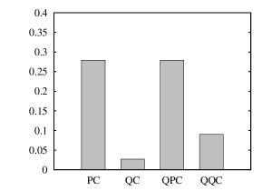
Figure 5: Information gain by the one-count process in the two-state model. PC, QC, QPC, and QQC denote the conventional photon counter, quantum counter, QND photon counter, and QND quantum counter, respectively.

The conventional photon counter and the QND photon counter provide the same amount of information in the two-state model. However, if the photon field is in an arbitrary superposition of the three states $|0\rangle$, $|1\rangle$, and $|2\rangle$, a numerical calculation shows that the QND photon counter provides more information than the conventional photon counter. Therefore, the QND photon counter has an advantage in terms of information gain. In contrast, the quantum counter provides about $10$ times less information than the QND photon counter. On the other hand, Fig. 6 displays the fidelity after the one-count process for each counter, namely, Eqs. (47), (75), (107), and (139).

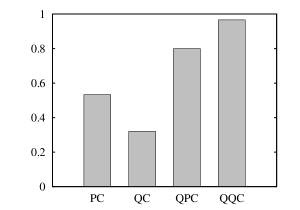
Figure 6: Fidelity after the one-count process in the two-state model. PC, QC, QPC, and QQC denote the conventional photon counter, quantum counter, QND photon counter, and QND quantum counter, respectively.

The QND versions change the state of the photon field less than that changed by their original versions. In particular, the QND quantum counter almost retains the state of photon field, compared with the quantum counter. To emphasize this property, we define an efficiency of counter by the ratio of information gain to fidelity loss, e.g., for the conventional photon counter

$$E^{\text{PC}}(1)\equiv\frac{I^{\text{PC}}(1)}{1-F^{\text{PC}}(1)},$$ (144)

and so on. Then, the QND quantum counter has approximately twice the efficiency of the QND photon counter, as shown in Fig. 7.

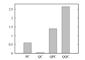
Figure 7: Efficiency of the one-count process in the two-state model. PC, QC, QPC, and QQC denote the conventional photon counter, quantum counter, QND photon counter, and QND quantum counter, respectively.

Figure 8 displays the physical reversibility of the one-count process of each counter, namely, Eqs. (49), (77), (109), and (141).

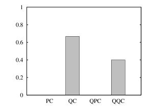
Figure 8: Physical reversibility of the one-count process in the two-state model. PC, QC, QPC, and QQC denote the conventional photon counter, quantum counter, QND photon counter, and QND quantum counter, respectively.

We can see that the quantum counter is the most reversible counter, while the conventional photon counter and the QND photon counter are irreversible.

Our results suggest that the reversibility of a counter tends to decrease the amount of information obtained by the counter. A similar result was shown [24] using reversible spin-$1/2$ measurement [11]. However, the reversibility of a counter does not necessarily decrease the state change caused by the counter. In fact, the quantum counter has the highest reversibility and provides the smallest amount of information but changes the state of the photon field most. This is because of a unitary part of the measurement operator [35, 23]. Note that the measurement operator $\hat{L}_{1}$ in Eq. (52) could be written by polar decomposition as

$$\hat{L}_{1}=\gamma\,\hat{U}\sqrt{\hat{a}\hat{a}^{\dagger}},$$ (145)

where $\hat{U}$ is a unitary operator and $\sqrt{\hat{a}\hat{a}^{\dagger}}$ is a non-negative operator, as long as the Hilbert space of the photon field is truncated to finite dimensions [36], as in the two-state model. The unitary part $\hat{U}$ causes an additional state change after the raw measurement $\sqrt{\hat{a}\hat{a}^{\dagger}}$, leaving the information gain and physical reversibility invariant. Therefore, the highest reversibility with the least information does not imply high fidelity in the quantum counter. Among the other counters, the conventional photon counter (11) also has such a unitary part, while the remaining two counters do not have a unitary part. A general theory on the relations among information, fidelity, and reversibility would be developed elsewhere.

We could implement the QND quantum counter proposed in Sec. 6 using a joint measurement. Consider performing the first measurement by the quantum counter and the second measurement by the conventional photon counter. If both the counters detect photons, the total process of the joint measurement is equivalent to the one-count process of the QND quantum counter because of

$$\hat{M}_{1}\hat{L}_{1}\propto\hat{Q}_{1}$$ (146)

from Eqs. (11), (52), and (112). The joint measurement is thus an implementation of the QND quantum counter, even though there are four possible outcomes. Note that this implementation is an example of the Hermitian conjugate measurement scheme [23], since the second measurement by the conventional photon counter is a Hermitian conjugate measurement of the first measurement by the quantum counter owing to $\hat{M}_{1}\propto\hat{L}_{1}^{\dagger}$. Therefore, the second measurement cancels the unitary part $\hat{U}$ of the measurement operator $\hat{L}_{1}$, thereby increasing the fidelity and information gain to the extent of a single measurement by the QND quantum counter.

References

- [1] M. A. Nielsen and I. L. Chuang, Quantum Computation and Quantum Information (Cambridge University Press, Cambridge, 2000).
- [2] C. H. Bennett and G. Brassard, in Proceedings of IEEE International Conference on Computers, Systems and Signal Processing, Bangalore, India (IEEE, New York, 1984), pp. 175–179.
- [3] A. K. Ekert, Phys. Rev. Lett. 67, 661 (1991).
- [4] C. H. Bennett, Phys. Rev. Lett. 68, 3121 (1992).
- [5] C. H. Bennett, G. Brassard, and N. D. Mermin, Phys. Rev. Lett. 68, 557 (1992).
- [6] M. Ueda and M. Kitagawa, Phys. Rev. Lett. 68, 3424 (1992).
- [7] M. Ueda, N. Imoto, and H. Nagaoka, Phys. Rev. A 53, 3808 (1996).
- [8] L. D. Landau and E. M. Lifshitz, Quantum Mechanics (Non-Relativistic Theory), 3rd ed. (Butterworth-Heinemann, Oxford, 1977).
- [9] M. Ueda, in Frontiers in Quantum Physics: Proceedings of the International Conference on Frontiers in Quantum Physics, Kuala Lumpur, Malaysia, 1997, edited by S. C. Lim, R. Abd-Shukor, and K. H. Kwek (Springer-Verlag, Singapore, 1999), pp. 136–144.
- [10] A. Imamoḡlu, Phys. Rev. A 47, R4577 (1993).
- [11] A. Royer, Phys. Rev. Lett. 73, 913 (1994); 74, 1040(E) (1995).
- [12] H. Terashima and M. Ueda, Phys. Rev. A 74, 012102 (2006).
- [13] A. N. Korotkov and A. N. Jordan, Phys. Rev. Lett. 97, 166805 (2006).
- [14] H. Terashima and M. Ueda, Phys. Rev. A 75, 052323 (2007).
- [15] Q. Sun, M. Al-Amri, and M. S. Zubairy, Phys. Rev. A 80, 033838 (2009).
- [16] Y.-Y. Xu and F. Zhou, Commun. Theor. Phys. 53, 469 (2010).
- [17] M. Koashi and M. Ueda, Phys. Rev. Lett. 82, 2598 (1999).
- [18] H. Terashima and M. Ueda, Int. J. Quantum Inf. 3, 633 (2005).
- [19] N. Katz, M. Neeley, M. Ansmann, R. C. Bialczak, M. Hofheinz, E. Lucero, A. O’Connell, H. Wang, A. N. Cleland, J. M. Martinis, and A. N. Korotkov, Phys. Rev. Lett. 101, 200401 (2008).
- [20] Y.-S. Kim, Y.-W. Cho, Y.-S. Ra, and Y.-H. Kim, Opt. Express 17, 11978 (2009).
- [21] H. Mabuchi and P. Zoller, Phys. Rev. Lett. 76, 3108 (1996).
- [22] M. A. Nielsen and C. M. Caves, Phys. Rev. A 55, 2547 (1997).
- [23] H. Terashima and M. Ueda, Phys. Rev. A 81, 012110 (2010).
- [24] M. Ban, J. Phys. A: Math. Gen. 34, 9669 (2001).
- [25] G. M. D’Ariano, Fortschr. Phys. 51, 318 (2003).
- [26] N. Bloembergen, Phys. Rev. Lett. 2, 84 (1959).
- [27] L. Mandel, Phys. Rev. 152, 438 (1966).
- [28] V. B. Braginsky and F. Y. Khalili, Rev. Mod. Phys. 68, 1 (1996), and references therein.
- [29] A. Uhlmann, Rep. Math. Phys. 9, 273 (1976).
- [30] E. B. Davies and J. T. Lewis, Commun. Math. Phys. 17, 239 (1970).
- [31] M. D. Srinivas and E. B. Davies, Opt. Acta 28, 981 (1981).
- [32] M. Ueda, N. Imoto, and T. Ogawa, Phys. Rev. A 41, 3891 (1990).
- [33] K. Usami, Y. Nambu, B.-S. Shi, A. Tomita, and K. Nakamura, Phys. Rev. Lett. 92, 113601 (2004); K. Usami, A. Tomita, and K. Nakamura, Int. J. Quantum Inf. 2, 101 (2004).
- [34] M. Ueda, N. Imoto, H. Nagaoka, and T. Ogawa, Phys. Rev. A 46, 2859 (1992).
- [35] C. A. Fuchs and K. Jacobs, Phys. Rev. A 63, 062305 (2001).
- [36] In the infinite-dimensional Hilbert space spanned by all the photon-number states with , the creation operator and annihilation operator do not have the polar decomposition: K. Fujikawa, Phys. Rev. A 52, 3299 (1995).