The classicality and quantumness of a quantum ensemble

Abstract

In this paper, we investigate the classicality and quantumness of a quantum ensemble. We define a quantity called ensemble classicality based on classical cloning strategy (ECCC) to characterize how classical a quantum ensemble is. An ensemble of commuting states has a unit ECCC, while a general ensemble can have a ECCC less than 1. We also study how quantum an ensemble is by defining a related quantity called quantumness. We find that the classicality of an ensemble is closely related to how perfectly the ensemble can be cloned, and that the quantumness of the ensemble used in a quantum key distribution (QKD) protocol is exactly the attainable lower bound of the error rate in the sifted key.

1 Introduction

Quantum theory has revealed many counterintuitive features of quantum systems in comparison with those of classical systems. The state of a classical system can be copied, deleted or distinguished with a unit probability, while an unknown quantum state can never be perfectly copied or deleted  [1, 2, 3], and non-orthogonal quantum states cannot be reliably distinguished [4, 5]. The no-cloning theorem assures the security of quantum key distribution protocols [6] and prohibits superluminal communication[7]. Non-commuting observables in quantum mechanics cannot be determined simultaneously, and a quantum measurement usually disturbs the involved quantum systems, in striking contrast to the fact that measurements can leave classical systems unperturbed in principle.

In this paper, we study the classicality and quantumness of a quantum ensemble $\mathcal{E}=\{q_{i},\rho_{i}\}$, specified by the set of states $\rho_{i}$ and the corresponding probabilities $p_{i}$. Some quantum ensembles can be manipulated like classical ones, whereas others can not. For example, an unknown state from an ensemble $\mathcal{E}_{ort}$ consisting of orthogonal pure states could be cloned perfectly and determined without being disturbed; on the other hand, a state from an ensemble $\mathcal{E}_{non}$ consisting of non-orthogonal states cannot be cloned perfectly and determined exactly [8]. By classicality, we mean how well a quantum ensemble can be manipulated as a classical one. Perfect clonability and distinguishability are essential characteristics of classical sets of states. Intuitively, the ensemble $\mathcal{E}_{ort}$ is more classical than $\mathcal{E}_{non}$, so the following questions naturally arise: what kind of ensembles could be handled like classical ones and what kind could not? Is there a quantity to quantify how classical an ensemble is? There have already been some researches on the quantumness of quantum ensembles [9, 10, 11, 12]. In this paper, we study the classicality and quantumness of a quantum ensemble from a different perspective. We start from considering how precisely an unknown state from the ensemble can be cloned and how stable it is under an appropriate measurement, i.e., how close the state after the measurement is to the original one.

For an arbitrary unknown input state $\rho$, a universal perfect cloning process does not exist, and many approximate cloning strategies have been proposed. One interesting strategy is given by the unitary transformation $|j\rangle|0\rangle\to|j\rangle|j\rangle$, where $\{\left|j\right\rangle\}$ is a basis of the Hilbert space of the input system and $|0\rangle$ is a blank state of an ancillary system. This cloning strategy was first introduced in [1], and we call it a classical cloning strategy under basis $\{\left|j\right\rangle\}$ as it is the quantum counterpart of the cloning process in the classical world.

Obviously, this classical cloning strategy is neither perfect nor optimum for cloning an unknown quantum state. The copies produced are generally different from the original state, so it is meaningful to quantify the distance between a copy and the original state. The way to measure the distance is investigated intensively and many proposals have been put forward [4, 13]. One distance measure is the relative entropy [12, 13], which has been used to quantify entanglement and correlations [13, 14, 15]. However, the relative entropy is not a genuine metric as it is not symmetric. Two other widely used distance measures, the trace distance and the fidelity [4], are well defined because both of them are symmetric and satisfy the requirements of good distance measures. In this paper, we use fidelity as the distance measure. The fidelity of $\rho$ and $\sigma$ is defined as [16]

$$F(\rho,\sigma)=(\mathrm{tr}{\sqrt{{\rho}^{1/2}\sigma{\rho}^{1/2}}})^{2}.$$ (1)

(The square root of the above quantity is also frequently used as the fidelity  [4], but we adopt Eq. (1) as the fidelity definition throughout this paper.) It is obvious that $0\leq F(\rho,\sigma)\leq 1$ and $F(\rho,\sigma)=1$ if and only if $\rho=\sigma$.

2 The ensemble classicality based on classical cloning strategy

For an ensemble $\mathcal{E}=\{q_{i},\rho_{i}\}$ consisting of the set of states $\{\rho_{i}\}$ and the corresponding probabilities of occurrence $\{p_{i}\}$, we investigate its classicality by studying how well an unknown state from the ensemble can be cloned by the classical cloning strategy under the basis $\{|j\rangle\}$. First, we define the average cloning fidelity for the ensemble $\mathcal{E}$ as

$$F_{ave}(\mathcal{E},\{|j\rangle\})=\sum_{i}q_{i}F(\rho_{i},\rho_{i}^{\prime}),$$ (2)

where $\rho_{i}^{\prime}$ is the state of an output copy via the classical cloning strategy under basis $\{\left|j\right\rangle\}$ if the input state is $\rho_{i}$, i.e.,

$$\rho_{i}^{\prime}=\mathrm{Tr}_{2}\sum_{i,j}\langle i|\rho_{i}|j\rangle|i\rangle|i\rangle\langle j|\langle j|=\sum_{j}\langle j|\rho_{i}|j\rangle|j\rangle\langle j|.$$ (3)

For an ensemble of orthogonal pure states, an average cloning fidelity 1 could be reached only if the states in the ensemble are actually the cloning basis states. For a general quantum ensemble $\mathcal{E}=\{q_{i},\rho_{i}\}$, it can be seen that $F_{ave}\leq 1$ as $F(\rho_{i},\rho_{i}^{\prime})\leq 1$ and $\sum_{i}q_{i}=1$. The average cloning fidelity $F_{ave}$ represents the performance of a classical copying strategy on a quantum ensemble; meanwhile, $F_{ave}$ can also represent stability of the states in an ensemble under a projective measurement, since $\rho_{i}^{\prime}=\sum_{j}\langle j|\rho_{i}|j\rangle|j\rangle\langle j|$ is also the density matrix after a von Neumann measurement on $\rho_{i}$ along the basis $\{|j\rangle\}$. In this sense, the average cloning fidelity characterizes how classical the ensemble is. Therefore, we define a quantity $J$, the ensemble classicality based on classical cloning strategy (ECCC), to quantify how classical the quantum ensemble $\mathcal{E}=\{q_{i},\rho_{i}\}$ is,

$$J(\mathcal{E})=\max_{\{|j\rangle\}}\{F_{ave}(\mathcal{E},|j\rangle)\}=\max_{\{|j\rangle\}}\{\sum_{i}q_{i}F(\rho_{i},\rho_{i}^{\prime})\},$$ (4)

where $\{|j\rangle\}$ is an orthonormal basis of the subspace spanned by the states in the ensemble. For an infinite quantum ensemble $\mathcal{E}=\{f(\alpha),\rho(\alpha)\}$, the ECCC is similarly defined as

$$J(\mathcal{E})=\max_{\{|j\rangle\}}\int f(\alpha)F(\rho(\alpha),\rho(\alpha)^{\prime}){\mathrm{d}}\alpha,$$ (5)

where $\rho(\alpha)^{\prime}=\sum_{j}\langle j|\rho(\alpha)|j\rangle|j\rangle\langle j|$ is the state of an output copy for an input $\rho(\alpha)$ and $f(\alpha)$ is the probability distribution function satisfying $\int f(\alpha){\mathrm{d}}\alpha=1$. It can be seen that the $J(\mathcal{E})$ defined above is an intrinsic property of the ensemble, independent of the cloning basis. It is evident that $\mathcal{E}$ can be manipulated like a classical ensemble only if $J(\mathcal{E})=1$.

A single state $\rho$ can be considered as an ensemble consisting of just one state with unit probability. The ECCC of a single-state ensemble $\rho$ is equal to one, since the cloning basis states could be chosen as the eigenstates of $\rho$, then $\rho=\rho^{\prime}$, and thus $J=F(\rho,\rho^{\prime})=1$.

In the following, the properties of ECCC will be studied. The range of $J$ will be given in the first two theorems.

Theorem 1.

The ECCC of a general ensemble $\mathcal{E}$ of states in a $d$-dimensional Hilbert space has the following upper and lower bounds: (i) $J(\mathcal{E})\leq 1$, with $J(\mathcal{E})=1$ if and only if all quantum states in the ensemble commute with each other; and (ii) $J(\mathcal{E})>\frac{1}{d}$ for any ensemble $\mathcal{E}$, and $J(\mathcal{E})\geq\frac{1}{d}+q_{m}\frac{d-1}{d}\geq\frac{N+d-1}{Nd}$ for any finite ensemble $\mathcal{E}=\{q_{i},\rho_{i}|i=1,2,\cdots,N\}$ of $N$ states, where $q_{m}=max\{q_{1},\cdots,q_{N}\}$.

Proof of theorem 1 is given in appendix A. The inequality $\frac{1}{d}<J(\mathcal{E})\leq 1$ is also valid for an ensemble of infinite number of states. The lower bound $\frac{1}{d}$ is generally not achievable for finite or infinite ensembles. Before presenting attainable lower bounds for specific cases, we give the following lemma (its proof is given in appendix B), which will be used in proving theorem 2.

Lemma 1.

For any state $\rho$ of a qubit system, the classical cloning strategy is performed with respect to a basis $\{|e_{i}\rangle\}$ and the state of either output copy is denoted by $\rho^{\prime}$, we have the following inequality

$$F(\rho,\rho^{\prime})\geq\sum_{i=0}^{1}q_{i}F(|\psi_{i}\rangle,\rho_{i}^{\prime})=\sum_{i,j=0}^{1}q_{i}|\langle e_{j}|\psi_{i}\rangle|^{4},$$ (6)

where $\rho_{i}^{\prime}=\sum_{j=0}^{1}|\langle e_{j}|\psi_{i}\rangle|^{2}|e_{j}\rangle\langle e_{j}|$ is the state of an output copy for an input $|\psi_{i}\rangle$, and $\{q_{i},|\psi_{i}\rangle\}$ are the eigenvalues and eigenvectors of $\rho$. Here, the right hand side of the inequality is actually the average cloning fidelity of the eigen-ensemble $\mathcal{E}=\{q_{i},|\psi_{i}\rangle\}$ of $\rho$.

In the following theorem, we present a tighter and achievable lower bound ($\frac{2}{d+1}$) of the ECCC for two special cases.

Theorem 2.

(i) For an ensemble $\mathcal{E}$ of pure states in a $d$-dimensional Hilbert space, $\frac{2}{d+1}\leq J(\mathcal{E})\leq 1$.

(ii) For an ensemble $\mathcal{E}$ consisting of general (pure or mixed) states in a two-dimensional Hilbert space of a qubit system, $\frac{2}{3}\leq J(\mathcal{E})\leq 1$.

The proof is given in appendix C. The lower bounds are actually achieved by an infinite ensemble consisting equiprobably of all pure states in the respective Hilbert space (see appendix C).

The ECCC $J$ of an ensemble $\{q_{i},\rho_{i}\}$ quantifies the maximum average performance of cloning the states from the ensemble by a classical strategy, thus provides a measure of how classical the ensemble is. From another perspective, the quantity $J$ of an ensemble $\{q_{i},\rho_{i}\}$ also tells us to what extent the states in the ensemble commute. The ECCC of an ensemble of mutually commuting states is equal to $1$, this is also in accordance with the fact that commuting states could be broadcasted [17].

Theorem 3.

For the ensembles $\mathcal{E}_{A}=\{q_{i},\rho_{iA}\}$, $\mathcal{E}_{B}=\{q_{j},\rho_{jB}\}$, and $\mathcal{E}_{AB}=\{{q_{i}}{q_{j}},\rho_{iA}\otimes\rho_{jB}\}$, there is an inequality

$$J(\mathcal{E}_{AB})\geq J(\mathcal{E}_{A})J(\mathcal{E}_{B});$$ (7)

the inequality (7) is also valid for the infinite ensembles $\mathcal{E}_{A}=\{f(\alpha),\rho_{A}(\alpha)\}$, $\mathcal{E}_{B}=\{f(\beta),\rho_{B}(\beta)\}$, and $\mathcal{E}_{AB}=\{f(\alpha)f(\beta),\rho_{A}(\alpha)\otimes\rho_{B}(\beta)\}$.

Proof.

Assume that $\{|k\rangle_{A}\}$ and $\{|m\rangle_{B}\}$ are the bases of the systems $A$ and $B$ which maximize $\sum_{i}q_{i}F(\rho_{iA},\rho_{iA}^{\prime})$ and $\sum_{j}q_{j}F(\rho_{jB},\rho_{jB}^{\prime})$ respectively, then $J(\mathcal{E}_{A})=\sum_{i}q_{i}F(\rho_{iA},\rho_{iA}^{\prime})$, $J(\mathcal{E}_{B})=\sum_{j}q_{j}F(\rho_{jB},\rho_{jB}^{\prime})$, where $\rho_{iA}^{\prime}=\sum_{k}\langle k|\rho_{iA}|k\rangle|k\rangle\langle k|$ and $\rho_{jB}^{\prime}=\sum_{m}\langle m|\rho_{jB}|m\rangle|m\rangle\langle m|$. The basis $\{|k\rangle\otimes|m\rangle\}$ may not be optimal for $\mathcal{E}_{AB}$, so from the definition of $J$ we can get

$$\begin{split}J(\mathcal{E}_{AB})&=\max_{\{|l\rangle^{AB}\}}\{F_{ave}(\mathcal{E}_{AB},\{|l\rangle^{AB}\})\}\\ &\geq F_{ave}(\mathcal{E}_{AB},\{|k\rangle\otimes|m\rangle\})\\ &=\sum_{ij}q_{i}q_{j}F(\rho_{iA}\otimes\rho_{jB},\rho_{iA}^{\prime}\otimes\rho_{jB}^{\prime})\\ &=\sum_{ij}q_{i}q_{j}F(\rho_{iA},\rho_{iA}^{\prime})F(\rho_{jB},\rho_{jB}^{\prime})\\ &=J(\mathcal{E}_{A})J(\mathcal{E}_{B}).\end{split}$$ (8)

The proof for infinite ensembles is similar. ∎

In fact, we have not found any example for which $J(\mathcal{E}_{AB})$ is strictly greater than $J(\mathcal{E}_{A})J(\mathcal{E}_{B})$ so far, so it is an open question that whether $J(\mathcal{E}_{AB})=J(\mathcal{E}_{A})J(\mathcal{E}_{B})$ holds true for all ensembles $\mathcal{E}_{A}$, $\mathcal{E}_{B}$, $\mathcal{E}_{AB}$ defined in Theorem 3.

It is intuitive to suggest that for an arbitrary ensemble $\{p_{i},\rho_{i}\}$ and a standard state $|0\rangle\langle 0|$, there is an inequality $J(\{p_{i},\rho_{i}\otimes|0\rangle\langle 0|\})\geq J(\{p_{i},\rho_{i}\otimes\rho_{i}\})$, with equality if and only if all $\rho_{i}$ are commuting. However, we don’t know how to prove this conjecture.

We show that $J$ is invariant under unitary operations. For a finite ensemble $\mathcal{E}=\{q_{i},\rho_{i}\}$, after a unitary operation $U$, the ECCC of the new ensemble is given as

$$\begin{split}J(U\mathcal{E}U^{\dagger})&=\max_{\{|j\rangle\}}\{F_{ave}(U\mathcal{E}U^{\dagger},|j\rangle)\}\\ &=\max_{\{U|j\rangle\}}\{F_{ave}(U\mathcal{E}U^{\dagger},U|j\rangle)\}\\ &=\max_{\{U|j\rangle\}}\{\sum_{i}q_{i}F(U\rho_{i}U^{\dagger},\sum_{j}\langle j|\rho_{i}|j\rangle U|j\rangle\langle j|U^{\dagger})\}\\ &=\max_{\{|j\rangle\}}\{\sum_{i}q_{i}F(\rho_{i},\rho_{i}^{\prime})\}\\ &=J(\mathcal{E}).\end{split}$$ (9)

It is obvious that the above equality is also valid for infinite ensembles. Therefore, an ensemble $\mathcal{E}_{0}$ can be transformed to another ensemble $\mathcal{E}_{1}$ by a unitary operation only if they have the same ECCC, i.e., $J(\mathcal{E}_{0})=J(\mathcal{E}_{1})$.

As an example, we consider the set of states used in the BB84 protocol, and for any given $p$ ($0\leq p\leq 1$) we define an ensemble $\mathcal{E}(p)$ as the set of states $\{|0\rangle,|1\rangle,(|0\rangle+|1\rangle)/\sqrt{2},(|0\rangle-|1\rangle)/\sqrt{2}\}$ with different prior probabilities $\{p/2,p/2,(1-p)/2,(1-p)/2\}$. The ensemble used in the BB84 protocol is essentially $\mathcal{E}(p=0.5)$. A straightforward calculation yields the ECCC of the ensemble $\mathcal{E}(p)$ as

$$J(\mathcal{E}(p))=\frac{3}{4}+\frac{1}{4}|2p-1|.$$ (10)

For the two ensembles, $J(\mathcal{E}(0.9))$ and $J(\mathcal{E}(0.5))$, specified by two different values of $p$, one easily has $J(\mathcal{E}(0.9))=0.95$, and $J(\mathcal{E}(0.5))=0.75$. Although both ensembles include the same set of quantum states, the ensemble $\mathcal{E}(0.9)$ is much more classical than the ensemble $\mathcal{E}(0.5)$ according to our definition of classicality. This is also intuitively correct, as in the limit case $p\rightarrow 0$ or $p\rightarrow 1$, the ensemble $\mathcal{E}(p)$ becomes a purely classical ensemble. The ECCC $J$ of an ensemble $\mathcal{E}=\{p_{i},\rho_{i}\}$ is essentially the maximum average cloning fidelity under a classical cloning strategy, it depends on the set of prior probabilities $\{p_{i}\}$.

Next, we consider two specific ensembles with infinite number of states in two-dimensional Hilbert space. A general basis of the two dimensional Hilbert space can be conveniently written as: $|e_{1}\rangle=\cos(\theta_{1}/2)|0\rangle+\sin(\theta_{1}/2)e^{i\varphi_{1}}|1\rangle$ and $|e_{2}\rangle=\sin(\theta_{1}/2)|0\rangle-\cos(\theta_{1}/2)e^{i\varphi_{1}}|1\rangle$. The first infinite ensemble $\mathcal{E}_{bloch}$ we consider consists of pure states uniformly distributed on the Bloch sphere, i.e., $\mathcal{E}_{bloch}=\{1/{4\pi},\cos(\theta/2)|0\rangle+\sin(\theta/2)e^{i\varphi}|1\rangle\}$, where $\theta\in[0,\pi]$ and $\varphi\in[0,2\pi)$. The average cloning fidelity of this ensemble is $F_{ave}=2/3$ which is independent of the basis used in the classical cloning process, so $J(\mathcal{E}_{bloch})=2/3$. The other ensemble we consider, a symmetric double-circle ensemble, is defined for a fixed $\theta$ as $\mathcal{E}(\theta)=\{1/{4\pi},\cos(\theta/2)|0\rangle\pm\sin(\theta/2)e^{i\varphi}|1\rangle\}$, where $\varphi\in[0,2\pi)$. The states in the ensemble $\mathcal{E}(\theta)$ lie on two symmetric latitudinal circles of the Bloch sphere with polar angles $\pm\theta$. The average cloning fidelity of this ensemble is $F_{ave}(\theta,\theta_{1},\varphi_{1})=1-{\sin^{2}\theta}/{2}+{\sin^{2}\theta_{1}}(3{\sin^{2}\theta}-2)/4$. According to the definition of $J$, we have

$$\begin{split}J(\theta)=&\max_{\{\theta_{1},\varphi_{1}\}}\{F_{ave}(\theta,\theta_{1},\varphi_{1})\}\\ =&\left\{\begin{aligned} &1-\frac{1}{2}{\sin^{2}\theta}&\textrm{if $0\leq\sin\theta\leq\sqrt{2/3}$}\\ &\frac{1}{2}+\frac{1}{4}{\sin^{2}\theta}&\textrm{if $\sqrt{2/3}<\sin\theta\leq 1$}\end{aligned}.\right.\end{split}$$ (11)

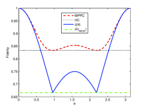
It can be seen that when $\theta=\arcsin(\sqrt{2/3})$ or $\pi-\arcsin(\sqrt{2/3})$, $J(\theta)$ reaches the minimal value $2/3$, which is also the ECCC of $\mathcal{E}_{bloch}$. When $\theta=\pi/2$, the states in the ensemble are equiprobably distributed on the $x-y$ equator, and the $J$ of this ensemble is $3/4$.

An unknown state cannot be perfectly cloned, but can be approximately cloned. The approximate cloning theories have been established and developed very well [7, 18, 19, 20]. In Fig. 1, the ECCC $J(\theta)$ of $\mathcal{E}(\theta)$ is depicted as a function of $\theta$, together with the ECCC $J(\mathcal{E}_{bloch})$ of the ensemble $\mathcal{E}_{bloch}$, the fidelity of the optimal mirror phase-covariant cloning (MPCC) [20], and the fidelity of universal cloning (UC) [19]. From Fig. 1, one can see that the MPCC fidelity $F(\theta)$ and the $J(\theta)$ reach their minimal values ($5/6$ and $2/3$ respectively) simultaneously when $\theta=\arcsin(\sqrt{2/3})$ or $\theta=\pi-\arcsin(\sqrt{2/3})$. The minimal value of the MPCC fidelity is equal to the UC fidelity, and the minimal value of $J(\theta)$ is equal to $J(\mathcal{E}_{bloch})$. Roughly speaking, Fig. 1 shows that the more classical an ensemble is, the more perfectly the states in the ensemble can be cloned. The ECCC $J$ of the ensembles used in the BB84 [6] protocol and in the six-state protocol [21, 22] are $3/4$ and $2/3$ respectively. It is interesting to note that the optimal cloning strategies for the BB84 ensemble and the six-state ensemble are equivalent to the optimal strategies for the phase-covariant cloning and the universal cloning respectively [7].

Figure 1: (Color online)The $\theta$ dependence of the ECCC and the cloning fidelilties for $\mathcal{E}(\theta)$ and $\mathcal{E}_{bloch}$: $J(\theta)$ (solid), $J(\mathcal{E}_{bloch})$ (dashdot), the MPPC (dashed), and the UC (dotted).

3 The quantumness of an ensemble

Next, we turn to study an opposite property of a quantum ensemble. We define the quantumness $Q$ of an ensemble $\mathcal{E}=\{q_{i},\rho_{i}\}$ as

$$Q(\mathcal{E})=1-J(\mathcal{E})=\min_{\{|j\rangle\}}\{\sum_{i}q_{i}(1-F(\rho_{i},\rho_{i}^{\prime}))\}.$$ (12)

The quantity $Q$ has similar properties to those of $J$. We have $0\leq Q<\frac{d-1}{d}$ for any ensemble, and $0\leq Q\leq(1-q_{m})(1-\frac{1}{d})\leq\frac{(N-1)(d-1)}{Nd}$ for any finite ensemble $\mathcal{E}=\{q_{i},\rho_{i}|i=1,2,\cdots,N\}$ of $N$ states, where $q_{m}=max\{q_{1},\cdots,q_{N}\}$. It can also be seen that $Q=0$ for a single-state ensemble or an ensemble of mutually commuting states, $Q\leq\frac{d-1}{d+1}$ for an ensemble of pure states, and $Q\leq\frac{1}{3}$ for an ensemble of states in a two-dimensional Hilbert space.

In [10], Fuchs et al. define a quantity $Q(S)$ to quantify the quantumness of a set of pure states by the difficulty of transmitting the states through a classical communication channel in the worst case. Recently, Luo et al. gave a quantity $Q_{D}$ to quantify the quantumness of an ensemble through the disturbances induced by von Neumann measurement [12]. Instead of the relative entropy which they used as the distance measure, we use the fidelity to measure the distance between the two states. Although both $Q_{D}$ and $Q$ are zero for the ensembles consisting of commuting states, they are different in general.

The quantumness $Q$ of an ensemble tells us the extent to which the ensemble is distinct from a purely classical ensemble, and we shall see that the quantumness of an ensemble used for quantum key distribution (QKD) is precisely the attainable lower bound of the error rate. In the quantum key distribution theory, the error rate is the rate of errors caused by eavesdroppers [23, 24]. Legitimate users can use it to detect whether there exist eavesdroppers. Now we study the relation between the quantumness of the ensemble used in a QKD protocol and the error rate under the intercept-resend eavesdropping strategies [24].

Theorem 4.

The quantumness $Q$ of the ensemble used in a general QKD protocol is the attainable lower bound of the error rate under the intercept-resend eavesdropping strategy.

Proof.

In a general QKD protocol, Alice sends a pure state $|\psi_{i}\rangle$ to Bob with a probability $q_{i}$, and the ensemble used is $\{q_{i},|\psi_{i}\rangle\}$. When Bob’s measurement basis is different from Alice’s sending basis, the state Bob receives is discarded, and when their bases are the same, the received state is reserved. The measurement results of the reserved states are usually called the sifted keys. The error rate is the average probability that Bob’s measurement gives a wrong result in the sifted key. With the intercept-resend strategy, the eavesdropper Eve intercepts a state from Alice, say $|\psi_{i}\rangle$, then performs a projective measurement along the basis $\{|j\rangle\}$ and gets an output $|j\rangle$ with a probability $|\langle j|\psi_{i}\rangle|^{2}$, and finally resends the output state to Bob. When Bob’s measurement basis is in accordance with Alice’s sending basis, the probability that Bob gets the original state $|\psi_{i}\rangle$ is $P=\sum_{j}|\langle j|\psi_{i}\rangle|^{4}=F(|\psi_{i}\rangle\langle\psi_{i}|,\rho_{i}^{\prime})$, where $\rho_{i}^{\prime}=\sum_{j}|\langle j|\psi_{i}\rangle|^{2}|j\rangle\langle j|$. Thus the error rate for this strategy is $R=\sum_{i}q_{i}(1-F(|\psi_{i}\rangle\langle\psi_{i}|,\rho_{i}^{\prime}))$. The quantumness of the ensemble $\{q_{i},|\psi_{i}\rangle\}$ is $Q=\min_{\{|j\rangle\}}\{\sum_{i}q_{i}(1-F(|\psi_{i}\rangle\langle\psi_{i}|,\rho_{i}^{\prime}))\}\leq R$. Therefore, the quantumness $Q$ is the lower bound of the error rate of a general QKD protocol, and the lower bound is achieved when the basis along which Eve performs the measurement is chosen as the basis that is used to achieve the ECCC of the ensemble $\{q_{i},|\psi_{i}\rangle\}$. ∎

It is obvious that an ensemble whose quantumness $Q$ is zero or very small is not suitable for QKD, since the eavesdropper can get the information of the keys without being detected. The quantumness $Q$ of an ensemble is closely related to the security of QKD protocol against the intercept-resend eavesdropping strategy. The error rates for BB84 protocol and six-state protocol are $1/4$ and $1/3$ respectively [23]. By simple calculation, we know that the quantumness of the two ensembles used in these two QKD protocols are $1/4$ and $1/3$ respectively, which are equal to their error rates. The quantumness of the six-state ensemble is $1/3$ which reaches the upper bound of the quantumness over all ensembles of qubit states. For the intercept-resend eavesdropping strategy, it can be seen that the six-state QKD protocol is most secure among the QKD protocols which use states in two-dimensional Hilbert space.

4 Conclusion

In conclusion, we have proposed a quantity $J$, the ensemble classicality based on classical cloning strategy (ECCC), to measure the classicality of a given ensemble. The quantity $J$ can tell how classical an ensemble is. When $J=1$ the ensemble behaves like a purely classical ensemble; and when $J<1$ the ensemble cannot be considered as a classical ensemble. We have revealed that the more classical an ensemble is, the better an unknown state from the ensemble can be cloned. The quantity of ECCC provides us with a tool to evaluate how well classical tasks such as cloning, deleting, and distinguishing could be accomplished for quantum ensembles. We also define the quantumness of an ensemble and we surprisingly find that the quantumness of an ensemble used in quantum key distribution is exactly the attainable lower bound of the error rate. Our work could be useful for further investigation of classical and quantum features of quantum ensembles and it could provide a quantitative framework for various tasks in quantum communication.

Appendix A: Proof of theorem 1

Proof.

(i) The upper bound can be easily shown since $J(\mathcal{E})=\max_{\{|j\rangle\}}\{\sum_{i}q_{i}F(\rho_{i},\rho_{i}^{\prime})\}\leq\sum_{i}q_{i}=1$ due to $F(\rho_{i},\rho_{i}^{\prime})\leq 1$. Now we prove that $J(\mathcal{E})=1$ if and only if all quantum states in the ensemble are mutually commutative. Suppose $\{|j^{*}\rangle\}$ is the basis that maximizes $F_{ave}$ for the ensemble $\mathcal{E}$. If $J(\mathcal{E})=1$, then for each $i$, $F(\rho_{i},\rho_{i}^{\prime})=1$ and thus $\rho_{i}=\rho_{i}^{\prime}=\sum_{j}\langle j^{*}|\rho_{i}|j^{*}\rangle|j^{*}\rangle\langle j^{*}|$. So all the states are diagonal in the same basis $\{|j^{*}\rangle\}$, and they commute with each other. On the other hand, if all the states in the ensemble commute with each other, all of them can be diagonalized simultaneously, i.e., there exists a basis in which all the states are diagonal and we can use this basis in the classical cloning strategy, then $\rho_{i}^{\prime}=\rho_{i}$ and $F(\rho_{i},\rho_{i}^{\prime})=1$ for each $i$, so we get $J(\mathcal{E})=1$.

(ii) Now we try to prove the lower bounds. Let $\rho_{m}$ be the state in the ensemble with the largest probability $q_{m}$, and $\{|e^{m}_{j}\rangle|j=1,\cdots,d\}$ be the orthonormal eigenstates of $\rho_{m}$. The classical cloning strategy could be performed with respect to the basis $\{|e^{m}_{j}\rangle|j=1,\cdots,d\}$, therefore $J(\mathcal{E})\geq\sum_{i}q_{i}F(\rho_{i},\rho_{i}^{\prime})$, where $\rho_{i}^{\prime}=\sum_{j}\langle e^{m}_{j}|\rho_{i}|e^{m}_{j}\rangle|e^{m}_{j}\rangle\langle e^{m}_{j}|$ and $F(\rho_{m},\rho_{m}^{\prime})=1$. The fidelity satisfies the inequality $F(\rho,\rho^{\prime})\geq\mathrm{tr}\rho\rho^{\prime}$ [16] for any two states $\rho$ and $\rho^{\prime}$, so $J(\mathcal{E})\geq\sum_{i\neq m}q_{i}\mathrm{tr}\rho_{i}\rho_{i}^{\prime}+q_{m}=\sum_{i\neq m}q_{i}\mathrm{tr}\rho_{i}^{\prime 2}+q_{m}$. Since $\rho_{i}^{\prime}$ is diagonal in the basis $\{|e^{m}_{j}\rangle|j=1,\cdots,d\}$, we have $\mathrm{tr}\rho_{i}^{\prime 2}=\sum_{j=1}^{d}(\rho_{i}^{\prime})_{jj}^{2}=\sum_{j=1}^{d}(\rho_{i})_{jj}^{2}\geq(\sum_{j=1}^{d}(\rho_{i})_{jj})^{2}/d=1/d$. Thus $J(\mathcal{E})\geq\sum_{i\neq m}q_{i}/d+q_{m}=1/d+q_{m}(d-1)/d\geq(N+d-1)/Nd$ since $q_{m}\geq 1/N$. This completes the proof.

∎

Appendix B: Proof of lemma 1

Proof.

A state $\rho$ in a two-dimensional Hilbert space has a spectral decomposition as $\rho=q_{0}|\psi_{0}\rangle\langle\psi_{0}|+q_{1}|\psi_{1}\rangle\langle\psi_{1}|$, where $|\psi_{0}\rangle$ and $|\psi_{1}\rangle$ are the orthonormal eigenstates of $\rho$. We choose the basis for a classical cloning strategy as $|e_{0}\rangle=\cos(\theta_{1}/2)|\psi_{0}\rangle+\sin(\theta_{1}/2)e^{i\varphi_{1}}|\psi_{1}\rangle$ and $|e_{1}\rangle=\sin(\theta_{1}/2)|\psi_{0}\rangle-\cos(\theta_{1}/2)e^{i\varphi_{1}}|\psi_{1}\rangle$. The output state from the classical cloning process is

$$\rho^{\prime}=\langle e_{0}|\rho|e_{0}\rangle|e_{0}\rangle\langle e_{0}|+\langle e_{1}|\rho|e_{1}\rangle|e_{1}\rangle\langle e_{1}|.$$ (13)

As $\rho$ can be written as $\rho=(I+\bm{r}\cdot\bm{\sigma})/2$ [4], where $\bm{r}$ is a real three-dimensional vector, $0\leq|\bm{r}|\leq 1$, and $\bm{\sigma}=(\sigma_{x},\sigma_{y},\sigma_{z})$. Similarly, we write $\rho^{\prime}=(I+\bm{r}^{\prime}\cdot\bm{\sigma})/2$. Using eq. (10) given in  [16], we get

$$\begin{split}F(\rho,\rho^{\prime})&=\frac{1}{2}\{1+\bm{r}\cdot\bm{r}^{\prime}+[(1-\bm{r}\cdot\bm{r})(1-\bm{r}^{\prime}\cdot\bm{r}^{\prime})]^{1/2}\}\\ &=\frac{1}{2}\{1+(q_{0}-q_{1})^{2}\cos^{2}\theta_{1}\\ &+[(1-(q_{0}-q_{1})^{2})(1-(q_{0}-q_{1})^{2}\cos^{2}\theta_{1})]^{1/2}\}.\end{split}$$ (14)

Let $\rho_{0}^{\prime}=\sum_{i=0}^{1}|\langle e_{i}|\psi_{0}\rangle|^{2}|e_{j}\rangle\langle e_{j}|$ and $\rho_{1}^{\prime}=\sum_{j=0}^{1}|\langle e_{j}|\psi_{1}\rangle|^{2}|e_{j}\rangle\langle e_{j}|$, then

$$\begin{split}\sum_{i=0}^{1}q_{i}F(|\psi_{i}\rangle\langle\psi_{i}|,\rho_{i}^{\prime})&=\sum_{i,j=0}^{1}q_{i}|\langle e_{j}|\psi_{i}\rangle|^{4}\\ &=1-\frac{1}{2}\sin^{2}\theta_{1}\end{split}$$ (15)

Thus,

$$\begin{split}F(\rho,\rho^{\prime})-&\sum_{i=0}^{1}q_{i}F(|\psi_{i}\rangle\langle\psi_{i}|,\rho_{i}^{\prime})\\ &\geq\frac{1}{2}\sin^{2}\theta_{1}(1-(q_{0}-q_{1})^{2})\geq 0\end{split}.$$ (16)

This completes the proof of Lemma 1. ∎

Appendix C: Proof of theorem 2

Proof.

(i) For an ensemble $\mathcal{E}=\{q_{i},|\psi_{i}\rangle\}$ of pure states, $J=max_{\{|j\rangle\}}\{\sum_{i}q_{i}F(|\psi_{i}\rangle,\rho_{i}^{\prime})\}=max_{\{|j\rangle\}}\{\sum_{ij}q_{i}|\langle j|\psi_{i}\rangle|^{4}\}$, where $\rho_{i}^{\prime}=\sum_{j}|\langle j|\psi_{i}\rangle|^{2}|j\rangle\langle j|$. $\rho_{i}^{\prime}$ is also the density matrix after the projective measurement on $|\psi_{i}\rangle$ along the basis $\{|j\rangle\}$. By the definition of $J$ we get $J\geq\overline{F_{ave}(\mathcal{E})}$, where the average is over all projective measurements, with respect to the unitarily invariant measure [11]. For any fixed state $|\psi\rangle$, one can prove that  [10, 25]

$$\int|\langle\phi|\psi\rangle|^{2n}\mathrm{d}\Omega_{\phi}=\frac{\Gamma(d)\Gamma(1+n)}{\Gamma(1)\Gamma(d+n)}$$ (17)

where the integral is over all pure states $\phi$ in a $d$ dimensional Hilbert space with respect to the unitarily invariant measure $\mathrm{d}\Omega_{\phi}$ on the pure states, and $\Gamma(x)$ is the Gamma function. So we get that

$$\begin{split}&J\geq\overline{F_{ave}(\mathcal{E})}=\overline{\sum_{ij}q_{i}|\langle j|\psi_{i}\rangle|^{4}}\\ &=d\sum_{i}q_{i}\int|\langle\phi|\psi_{i}\rangle|^{4}\mathrm{d}\Omega_{\phi}=d\sum_{i}q_{i}\frac{\Gamma(d)\Gamma(3)}{\Gamma(1)\Gamma(d+2)}\\ &=\frac{2}{d+1}.\end{split}$$ (18)

From above derivation, one can easily see that the lower bound is actually achieved by an infinite ensemble consisting equiprobably of all pure states in a $d$-dimensional Hilbert space.

(ii) For a two dimensional states ensemble, from Lemma 1,

$$\begin{split}J=&\max_{\{|e_{j}\rangle\}}\{\sum_{ik}q_{i}F(\rho_{i},\rho_{i}^{\prime})\}\\ &\geq\max_{\{|e_{j}\rangle\}}\{\sum_{ik}q_{i}q_{ik}F(|\psi_{ik}\rangle,\rho_{ik}^{\prime})\}\\ &=\max_{\{|e_{j}\rangle\}}\{\sum_{ik}q_{i}q_{ik}|\langle e_{j}|\psi_{ik}\rangle|^{4}\}\\ &\geq\sum_{ik}q_{i}q_{ik}\;\overline{|\langle e_{j}|\psi_{ik}\rangle|^{4}},\end{split}$$ (19)

where $\{q_{ik},|\psi_{ik}\rangle\}$ are the eigenvalues and corresponding eigenvectors of $\rho_{i}$, and the average is over all projective measurements $\{|e_{j}\rangle\langle e_{j}|\}$. From Eq. (17), we get

$$J\geq\frac{2}{3}\sum_{ik}q_{i}q_{ik}=\frac{2}{3}.$$ (20)

The lower bound is achieved by an infinite ensemble consisting equiprobably of all pure states on the Bloch sphere. ∎

References

- [1] W. K. Wootters and W. H. Zurek, Nature(London) 299 (1982) 802-803.
- [2] D. Dieks, Phys. Lett. A 92 (1982) 271-272.
- [3] A. K. Pati and S. L. Braunstein, Nature(London) 404 (2000) 164-165.
- [4] M. A. Nielsen and I. Chuang, Quntum Computation and Quantum Information, Cambridge University Press, Cambridge (2000).
- [5] S. Pang and S. Wu, Phys. Rev. A 80 (2009) 052320.
- [6] C. H. Bennett and G. Brassard, in Proceedings of the IEEE International Conference on Computers, Systems and Signal Processing, Bangalore, India(1984), pp. 175-179.
- [7] V. Scarani, S. Iblisdir, N. Gisin, and A. Acin, Rev. Mod. Phys. 77 (2005) 1225-1256.
- [8] S. Massar, S. Popescu, Phys. Rev. Lett. 74 (1995) 1259-1263.
- [9] C. A. Fuchs quant-ph/9810032 (1998); M. Horodecki, P. Horodecki, R. Horodecki, M. Piani quant-ph/0506174 (2005).
- [10] C. A. Fuchs and M.Sasaki, Quant. Inf. Comput. 3 (2003) 377-404.
- [11] C. A. Fuchs, Quant. Inf. Comput 4 (2004) 467-478.
- [12] S. Luo, N. Li, and W. Sun, Quantum. Inf. Process. 9 (2010) 711-726.
- [13] V. Vedral, Rev. Mod. Phys. 74 (2002) 197-234.
- [14] V. Vedral, M. A. Plenio, M. A. Rippin, and P. L. Knight, Phys. Rev. Lett. 78 (1997) 2275-2279.
- [15] K. Modi, T. Paterek, W. Son, V. Vedral, and M. Williamson, Phys. Rev. Lett. 104 (2010) 080501.
- [16] R. Jozsa, J. Mod. Opt. 41 (1994) 2315-2323.
- [17] H. Barnum, C. M. Caves, C. A. Fuchs, R. Jozsa, and B. Schumacher, Phys. Rev. Lett. 76 (1996) 2818-2821.
- [18] D. Bruß, M. Cinchetti, G. M. D’Ariano, and C. Macchiavello, Phys. Rev. A 62 (2000) 012302.
- [19] V. Bužek, M. Hillery, Phys. Rev. A 54 (1996) 1844-1847.
- [20] K. Bartkiewicz, A. Miranowicz, and S. K. Ozdemir, Phys. Rev. A 80 (2009) 032306.
- [21] D. Bruß, Phys. Rev. Lett. 81 (1998) 3018-3021.
- [22] H. Bechmann-Pasquinucci and N. Gin, Phys. Rev. A 59 (1999) 032306.
- [23] N. Gisin, G. Ribordy, W. Tittel, and H. Zbinden, Rev. Mod. Phys. 74 (2002) 145-195.
- [24] B. Huttner and A. Ekert, J. Mod. Opt. 46 (1994) 2455-2466.
- [25] K. R. Jones, Phys. Rev. A 50 (1994) 3682-3699.