Fluid dynamics and jamming in a dilatant fluid

Abstract

We present a phenomenological fluid dynamics model for a dilatant fluid, i.e. a severe shear thickening fluid, by introducing a state variable. The Navier-Stokes equation is coupled with the state variable field, which evolves in response to the local shear stress as the fluid is sheared. The viscosity is assumed to depend upon the state variable and to diverge at a certain value due to jamming. We demonstrate that the coupling of the fluid dynamics with the shear thickening leads to an oscillatory instability in the shear flow. The model also shows a peculiar response of the fluid to a strong external impact.

Dense mixture of starch and water is an ideal material to demonstrate the shear thickening property of the non-Newtonian fluid. It may behave as liquid but is immediately solidified upon sudden application of stress, thus one can even run over the pool filled with the fluid. It is amazing to see that it develops protrusions sticking out of the surface when it is subject to strong vertical vibrationMerkt et al. (2004); Ebata et al. (2009), and also intriguing that the fluid vibrates spontaneously when one simply pours it out of a container. A source of these unusual behaviors is the severe shear thickening; the viscosity increases almost discontinuously by orders of magnitude at a certain critical shear rateFall et al. (2008), which makes the fluid behave like a solid upon abrupt deformation. Such severe shear thickening is often found in dense colloid suspensions and granule-fluid mixturesHoffman (1972); Barnes (1989); Brown and Jaeger (2009); Laun et al. (1991), and they have been sometimes called “dilatant fluid” due to the apparent analogy to Reynolds dilatancy of granular mediaReynolds (1885).

Despite its suggestive name, physicists have not reached the microscopic understanding of this shear thickening property. It was originally proposed that the shear thickening is due to the order-disorder transition of dispersed particlesHoffman (1972, 1974, 1998); Barnes (1989); the viscosity increases when the fluid flow in high shear regime destroys the layered structure that has appeared in lower shear rate regime. Although there seem to be some situations where this mechanism was believed to cause the shear thickening, there are other cases where the layered structure is not observed prior to the shear thickeningLaun et al. (1992) or no significant changes in the particle ordering are found upon the discontinuous thickeningMaranzano and Wagner (2002); Egres and Wagner (2005). The cluster formation due to hydrodynamic interactionBrady and Bossis (1985); Bender and Wagner (1996); Maranzano and Wagner (2001); Melrose and Ball (2004a) and the jammingMelrose and Ball (2004b); Farr et al. (1997); Cates et al. (1998); Bertrand et al. (2002); Lootens et al. (2005); Fall et al. (2008); Brown and Jaeger (2009) have been proposed as plausible mechanisms.

There are several peculiar features in the shear thickening shown by a dilatant fluid: (i) the thickening is so severe and instantaneous that it might be used even to make a body armor to stop a bulletWagner and Brady (2009), (ii) the relaxation after removal of the external stress occurs within a few seconds, that is not very slow but not as instantaneous as in the thickening process, (iii) the thickened state is almost like a solid and does not allow much elastic deformation unlike a visco-elastic material, (iv) the viscosity shows hysteresis upon changing the shear rateLaun et al. (1991), (v) noisy fluctuations have been observed in response to an external shear stress in the thickening regimeLaun et al. (1991); Lootens et al. (2005).

In this report, we construct a phenomenological model in the macroscopic level and examine the fluid dynamical behavior of the dilatant fluid. We introduce a state variable that describes phenomenologically an internal state of the fluid, and couple its dynamics with the fluid dynamics. We find that the following two aspects of the model are important: (1) the fluid state changes in response to the shear stress, (2) the state variable changes with the rate proportional to the shear rate. We examine the model behavior in simple configurations and demonstrate that the model is capable of describing the characteristic features of hydrodynamic behavior and shows the oscillatory instability.

Model:

The model is based upon the incompressible Navier-Stokes equation with the viscosity $\eta(\phi)$ that depends upon the state variable $\phi$. The scaler field $\phi$, which takes a value in [0, 1], represents the local state of the medium. We assume two limiting states: the low viscosity state ($\phi\sim 0$) and the high viscosity state ($\phi\sim 1$). At $\phi=1$, the system is supposed to be jammed and the viscosity diverges.

The state variable $\phi$ relaxes to a steady value $\phi_{*}$ determined by the local shear stress $S$; $\phi_{*}$ is supposed to be a continuous and monotonically increasing from 0 to $\phi_{M}$ as a function of $S$ with a characteristic stress $S_{0}$. The limiting value $\phi_{M}$ represents the state of the medium in the high stress limit and should depend upon the medium properties such as the packing fraction of the dispersed granules. In the following, we employ the forms

$$\eta(\phi)=\eta_{0}\exp\left[{A\,\phi\over 1-\phi}\right],\quad\phi_{*}(S)=\phi_{M}{(S/S_{0})^{2}\over 1+(S/S_{0})^{2}}$$ (1)

with a dimensionless constant $A$. We assume the Vogel-Fulcher type strong divergence in $\eta(\phi)$ in oder to represent the severe thickening, but a detailed functional form is rather arbitrary.

For the simple shear flow configuration as in Fig.1(a) with the flow field $v$ given by $(u(z,t),0,0)$, the model is described by the following set of equations,

$$\rho{\partial u(z,t)\over\partial t} = {\partial\over\partial z}S(z,t),$$ (2)

$${\partial\phi(z,t)\over\partial t} = -{1\over\tau}\Bigl{(}\phi(z,t)-\phi_{*}(S(z,t))\Bigr{)},$$ (3)

with $\rho$ and $\tau$ being the medium density and the relaxation time. The shear stress $S(z,t)$ is given by

$$S(z,t)=\eta(\phi)\dot{\gamma},\qquad\dot{\gamma}\equiv{\partial u\over\partial z},$$ (4)

where the shear rate is denoted by $\dot{\gamma}$.

Now, we suppose the relaxation of $\phi$ toward $\phi_{*}$ is driven by the shear deformation, thus the relaxation rate $1/\tau$ is not constant but proportional to the absolute value of the shear rate, i.e.

$${1/\tau}={|\dot{\gamma}|/r}$$ (5)

with a dimensionless parameter $r$. Note that, with this form of relaxation, the state variable $\phi$ does not exceed 1 even when $\phi_{M}>1$ because $\dot{\gamma}=0$ at $\phi=1$ due to the diverging viscosity.

This particular form of relaxation is employed in order to represent the athermal relaxation driven by local deformation. The system responds in accordance with the deformation rate, and does not change the state when it does not deform. This is natural if we consider the state change is caused by local configurational changes of the dispersed granules in the situation where Brownian motion does not play an important role.

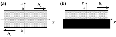
Figure 1: Simple shear flow configurations with the coordinate system.

Steady shear flow:

First, we examine the model behavior in the steady shear flow configuration with a fixed external stress $S_{\rm e}$. The boundary condition is then given by

$$S_{\rm e}=S(z,t)\Bigr{|}_{z=\pm h}.$$ (6)

The steady state solution for Eqs.(2) and (3) with this boundary condition is obtained easily as

$$\phi=\phi_{*}(S_{\rm e}),\quad\dot{\gamma}={S_{\rm e}\over\eta(\phi_{*})}\equiv\dot{\gamma}_{*}(S_{\rm e}).$$ (7)

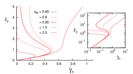
Figure 2: The stress-shear rate relation for the viscosity given by Eq.(1) with $A=1$. The inset shows the same plots in the logarithmic scale. We employ the unit system where $\eta_{0}=S_{0}=\rho=1$.

The stress-shear rate curves are plotted in Fig.2 for $\phi_{*}$ and $\eta(\phi)$ given by Eq.(1) with $A=1$ for various values of $\phi_{M}$. In the logarithmic scale, the straight line with the slope 1 corresponds to the linear stress-shear rate relation with a constant viscosity. In the curve for $\phi_{M}=0.8$, one can see the two regimes: the low viscosity regime and the high viscosity regime. Between the two regimes, there is an unstable region. From this stress-shear rate curve, we expect there should be hysteresis upon changing the shear rate $\dot{\gamma}$ with discontinuous jumps between the two branches. The jumps correspond to the discontinuous change of viscosity, i.e. the abrupt shear thickening. For the case $\phi_{M}\geq 1$, the curves do not have an upper linear branch because the viscosity diverges and the fluid is solidified.

Oscillation in the shear flow:

If the external stress $S_{\rm e}$ is kept at a value in the unstable branch, where

$${\partial\dot{\gamma}_{*}\over\partial S_{\rm e}}<0,$$ (8)

i.e. the shear rate decreases as the stress increases, the steady flow may become unstable. The linear stability analysis within the solution of the form $(u(z,t),0,0)$ shows that the mode whose wave number $k$ in the $z$-axis satisfies

$$0<k^{2}<\rho{\dot{\gamma}_{*}\over r}\left[-{\partial\dot{\gamma}_{*}\over\partial S_{\rm e}}\right]\equiv k_{\rm c}^{2}$$ (9)

grows and the threshold mode $k_{\rm c}$ oscillates at the finite frequency

$$\omega_{\rm c}=\sqrt{{S_{\rm e}\over\rho\,r}}\;k_{\rm c}.$$ (10)

Since the smallest possible wave number $k_{\rm min}$ is given by $k_{\rm min}=2\pi/4h$, we expect the oscillatory flow appears for $k_{\rm min}<k_{\rm c}$ as the system width increases if the external stress is in the unstable branch.

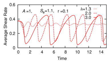
Figure 3: Oscillation of the average shear rate $u(h)/h$ in shear flow for $h=$1.3, 2, and 3 with $A=1$, $\phi_{M}=1$, $r=0.1$, and $S_{\rm e}=1.1$. The initial state is chosen as the steady solution (7) with $S_{\rm e}=1.0$ at $t=0$.

The oscillatory behavior of the shear flow in the unstable regime can be seen by numerically integrating Eqs.(2) and (3) with (6). In Fig.3, the average shear rate $u(h)/h$ is plotted as a function of time for some values of the system width $2h$ for $\phi_{M}=1$, $A=1$, and $r=0.1$ with the external shear stress $S_{\rm e}=1.1$ in the unstable regime. The initial state is chosen as the steady solution (7) with $S_{\rm e}=1$. For the case of $h=1.3$, one can see the overdamped oscillation that converges to the steady state, but for the larger values of $h$, the system undergoes the oscillatory transition and the surface velocity oscillates with an saw-tooth like wave profile, namely, the gradual increase of velocity followed by a sudden drop.

The time development of the spatial variations for the state variable $\phi$ and the velocity $u$ are plotted in Fig.4 for $h=2$. Only the positive halves ($z>0$) of the symmetric solutions are shown. One can see the high shear rate region gradually extends towards the center as $\phi$ relaxes, then the velocity drops suddenly to a very small value when the shear rate exceeds a certain value and $\phi$ increases rapidly. This sudden drop of velocity is due to the abrupt thickening of the fluid caused by the high shear stress. The resulting low shear rate eventually leads to the low shear stress, which in turn leads to small $\phi$ with low viscosity, then the shear rate starts increasing again.

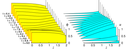
Figure 4: Spatial variation of shear flow oscillation for $A=1$, $\phi_{M}=1$, $r=0.1$, $S_{\rm e}=1.1$, and $h=2$.

Response to impact:

The athermal relaxation (5) gives the system an interesting feature in responding to an external impact. We consider the simple shear flow but assume the fixed lower boundary at $z=0$ and the upper boundary at $z=h$ is forced to move at the velocity $u_{0}$ at $t=0$ (Fig.1(b)). Then, the motion of the upper wall is given by the equation,

$$m{du(h,t)\over dt}=-\eta(\phi)\left.{\partial u\over\partial z}\right|_{z=h},$$ (11)

where $m$ is the mass of the upper wall per unit length.

Fig.5 shows the displacement $X$ of the upper wall,

$$X(t)=\int_{0}^{t}u(h,t^{\prime})dt^{\prime},$$ (12)

for the three cases, $\phi_{M}=$ 0.8, 1, and 2, for various initial speeds. The wall decelerates rapidly as the fluid thickens due to the imposed stress, and eventually stops. In the case of $\phi_{M}=0.8$, the total distance that the wall moves before it stops increases as the initial speed $u_{0}$. On the other hand, in the case of $\phi_{M}=2$, the total displacement does not depend on $u_{0}$. This is because the fluid jammed at a certain strain as it deforms, and cannot deform further.

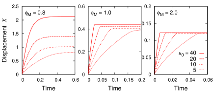
Figure 5: The time dependence of the displacement $X$ after the impact with the initial speed $u_{0}=$40, 20, 10, and 5 for the system with $\phi_{M}=0.8$, 1, and 2. The other parameters are $h=2$, $A=1$, $r=0.1$, and $m=1$.

Concluding remarks:

There are a couple of related models: the soft glassy rheology(SGR) modelHead et al. (2001) and the schematic mode coupling theory(MCT)Holmes et al. (2005). In the SGR model, SGR is extended to describe the shear thickening by introducing the stress dependent effective temperature, which may be compared with the inverse of the state variable $\phi$ of our model. In the schematic MCT, the jamming transition has been examined by means of MCT incorporating the effects of shear schematically. Both are semi-empirical but deal with microscopic processes and produce the similar flow curves as Fig.2. On the other hand, the present model is phenomenological one only for macroscopic description to study the interplay between the fluid dynamics and the shear thickening, which is embedded in Eqs.(1).

Although our model is phenomenological, the microscopic picture we may have for a dense mixture of granules and fluid is the following; in the low stress regime ($\phi\sim 0$), the particles are dispersed thus the medium can deform easily due to the lubrication, whereas, in the high stress regime ($\phi\sim 1$), the particles form contacts and force chains to support the stress, and eventually get jammed when the packing fraction is large enough (Fig.6). With this picture, it is natural to assume that the time scale for the state change is set by the shear rate in the case where the athermal deformation drives the configurational changes, and then the parameters $S_{0}$ and $r$ correspond to the stress and the strain, respectively, around which the neighboring granules start touching each other. In the case where the thermal relaxation takes place, the time scale may be given by

$${1\over\tau}={|\dot{\gamma}|\over r}+{1\over\tau_{\rm th}}\,,$$ (13)

where $\tau_{\rm th}$ is the time scale that the thermal agitation dislocates the contacts.

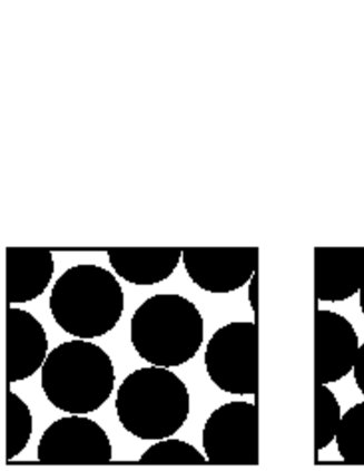
Figure 6: Schematic illustration of configurations for low stress (left) and high stress(right) regime.

We have assumed that the state is determined by the shear stress, but it is instructive to consider what would happen if the state is determined by the shear rate. If $\phi_{*}$ is a function of $\dot{\gamma}$ instead of Eq.(1), then the stress-shear rate curve becomes monotonically increasing without an unstable branch, thus there should be no discontinuity and hysteresis, thus no instability that leads to the oscillation. This suggests that experimentally observed discontinuous transitionFall et al. (2008) and the hysteresisLaun et al. (1991) can be attributed to the “shear-stress thickening” property of the medium. The direct consequence of the shear-stress thickening may be seen in the gravitational slope flow, where the flux does not increases monotonically as the inclination angle because the fluid becomes more viscous under larger shear stress, thus it may flow slower as the slope is inclined steeper.

A peculiar result of the present model is the oscillatory instability in the shear flow. Superficially, this might look like a stick-slip motion, but the physical origin is different; the stick-slip motion is caused by the slip weakening friction when the system is driven at a constant speed through an elastic device. If the present system is driven at a constant velocity, the system settles in one of the stable states for a given $\dot{\gamma}$. The oscillatory behavior in the present system appears under the drive with a constant shear stress, and it is a result of the coupling between the internal dynamics and the fluid dynamics. In this sense, it is also different from the oscillation in the SGR model, where the fluid dynamics is not considered. We found that the oscillatory flow also appears in the gravitational slope flow.

Regarding the oscillations in experiments, one can easily notice the vibration around 10 Hz when pouring the cornstarch-water mixture out of a cup. In the literature, the pronounced fluctuations in the deformation rate have been reported in the shear stress controlled experiment near the critical shear rateLaun et al. (1991); Lootens et al. (2005) and the pressure driven flow through microchannelsIsa et al. (2009), but not many experiments have been reported yet.

This work was supported by KAKENHI(21540418).

References

- Merkt et al. (2004) F. S. Merkt, R. D. Deegan, D. I. Goldman, E. C. Rericha, and H. L. Swinney, Phys. Rev. Lett. 92, 184501 (2004).
- Ebata et al. (2009) H. Ebata, S. Tatsumi, and M. Sano, Phys. Rev. E 79, 066308 (2009).
- Fall et al. (2008) A. Fall, N. Huang, F. Bertrand, G. Ovarlez, and D. Bonn, Phys. Rev. Lett. 100, 018301 (2008).
- Hoffman (1972) R. Hoffman, Trans. Soc. Rheol. 16, 155 (1972).
- Barnes (1989) H. Barnes, J. Rheology 33, 329 (1989).
- Brown and Jaeger (2009) E. Brown and H. M. Jaeger, Phys. Rev. Lett. 103, 086001 (2009).
- Laun et al. (1991) H. Laun, R. Bung, and F. Schmidt, J. Rheol. 35, 999 (1991).
- Reynolds (1885) O. Reynolds, Phil. Mag. S5, 469 (1885).
- Hoffman (1974) R. Hoffman, J. Colloid and Interface Sci. 46, 491 (1974).
- Hoffman (1998) R. Hoffman, J. Rheol. 42, 111 (1998).
- Laun et al. (1992) H. Laun, R. Bung, S. Hess, W. Loose, O. Hess, K. Hahn, E. Hädicke, R. Hingmann, and F. Schmidt, J. Rheol. 36, 943 (1992).
- Maranzano and Wagner (2002) B. J. Maranzano and N. J. Wagner, J. Chem. Phys. 117, 10291 (2002).
- Egres and Wagner (2005) R. G. Egres and N. J. Wagner, J. Rheol. 49, 719 (2005).
- Brady and Bossis (1985) J. Brady and G. Bossis, J. Fluid Mech. 155, 105 (1985).
- Bender and Wagner (1996) J. Bender and N. J. Wagner, J. Rheol. 40, 899 (1996).
- Maranzano and Wagner (2001) B. J. Maranzano and N. J. Wagner, J. Chem. Phys. 114, 10514 (2001).
- Melrose and Ball (2004a) J. Melrose and R. Ball, J. Rheol. 48, 937 (2004a).
- Melrose and Ball (2004b) J. Melrose and R. Ball, J. Rheol. 48, 961 (2004b).
- Farr et al. (1997) R. Farr, J. Melrose, and R. Ball, Phys. Rev. E 55, 7203 (1997).
- Cates et al. (1998) M. E. Cates, J. P. Wittmer, J.-P. Bouchaud, and P. Claudin, Phys. Rev. Lett. 81, 1841 (1998).
- Bertrand et al. (2002) E. Bertrand, J. Bibette, and V. Schmitt, Phys. Rev. E 66, 060401 (2002).
- Lootens et al. (2005) D. Lootens, H. van Damme, Y. Hémar, and P. Hébraud, Phys. Rev. Lett. 95, 268302 (2005).
- Wagner and Brady (2009) N. J. Wagner and J. F. Brady, Physics Today 62(10), 27 (2009).
- Head et al. (2001) D. A. Head, A. Ajdari, and M. E. Cates, Phys. Rev. E 64, 061509 (2001).
- Holmes et al. (2005) C. B. Holmes, M. E. Cates, M. Fuchs, and P. Sollich, J. Rheol. 49, 237 (2005).
- Isa et al. (2009) L. Isa, R. Besseling, A. N. Morozov, and W. C. K. Poon, Phys. Rev. Lett. 102, 058302 (2009). The oscillation is observed only in narrow channels of the width less than 30 particle diameters. This suggests the granule discreteness is essential, in which case the origin of the oscillation is different from our model.