Towards a unified characterization of phenological phases: fluctuations and correlations with temperature

Abstract

Phenological timing – i.e. the course of annually recurring development stages in nature – is of particular interest since it can be understood as a proxy for the climate at a specific region; moreover changes in the so called phenological phases can be a direct consequence of climate change. We analyze records of botanical phenology and study their fluctuations which we find to depend on the seasons. In contrast to previous studies, where typically trends in the phenology of individual species are estimated, we consider the ensemble of all available phases and propose a phenological index that characterizes the influence of climate on the multitude of botanical species.

(arxiv-version 01)

1 Introduction

Phenology is a well-known concept in ecology to describe the timing of certain periodical development stages of species throughout the year [1]. Developmental stages, or phases (e.g. flowering, fruit ripening, leaf coloring, foliation), have been studied over many decades in Europe using defined plant species. This information is often used to develop phenological calendars and describe natural seasons [2].

Phenological phases are sensitive to temperature [3, 4], and shifts of phases are often regarded as the first signs of a change in climate [5, 6, 7]. An average earlier onset of plant phases of $3.8$ days per $1$ ^∘C increase over the last decades has been observed for Europe, with negative shifts for spring and summer phases and positive shifts for fall phases [8].

A well-known phenological record is the cherry blossoming in Kyoto, Japan, which has advanced by $7$ days between 1971 and 2000 [9]. It has been shown that the flowering dates of closely related species in Japan have responded to climate change in a similar way [10]. Nevertheless, early flowering plants deviate from this trend, showing larger advances due to warming than later flowering species, which could result in an ecological mismatch in the future.

The reaction of plants to climatic changes is non-linear and not uniform [11, 12, 13]. It has been observed that while the correlation between air temperature and the onset of spring and summer plant phases is strong, the correlation becomes weaker for fall phases [14, 4, 3]. It is suggested that later in the year, other factors like water availability, nutrition and pollution gain in importance over the influence of temperature [8]. Moreover, the temporal and spatial variability of phenological trends differs between plants and is strongest for spring phases [15]. Differences in the phenological response to climate warming may also result from locally adapted species [16].

Large uncertainties remain about the future development of phenological phases. Several studies concentrate on the influence of temperature and, by assuming a linear relation between rising air temperature and changes in the phenological cycle, extrapolate possible future changes [17, 18]. Usually, this temperature sensitivity is analyzed by finding the best correlation for the preceding months of an onset date, see e.g. [19, 8, 20, 13]. While these previous studies concentrated on temperature responses of specific phases or groups of phases, no integrated approach assessing changes in the annual phenological cycle has been developed so far. We therefore propose a phenological index, which characterizes the annual phenological cycle by taking into account both the shift of spring phases and the shift of fall phases simultaneously. Following this approach, more general conclusions about climatic influences on phenology can be drawn since more data is used, implying better statistics, and an average prospect is obtained. The method is applied to the state North Rhine-Westphalia, Germany.

The paper is organized as follows. In Sec. 2 we present our concept of a phenological index. The data this work is based on is described in Sec. 3. The results of our analysis are given in Sec. 4 in three subsections regarding fluctuations, the phenological index, and correlations between the index and temperature records. In the last Section we discuss the results and give an outlook.

2 Method

Phenological events are referred to as phases, since they take place on a specific day of the year and occur at a more or less regular pace. For the phase $\phi_{p,t}$, i.e. the day of the year when the phenological event $p$ takes place in year $t$, and the average phase over all years, $\langle\phi\rangle_{p}$, we consider the phase anomaly

$$\varphi_{p,t}=\phi_{p,t}-\langle\phi\rangle_{p}\,,$$ (1)

where $\langle\cdot\rangle$ denotes the average over time and $\langle\phi\rangle$ is defined by $\tan\langle\phi\rangle:=\frac{\langle\sin\phi\rangle}{\langle\cos\phi\rangle}$ [21], see A. Accordingly, $\varphi_{p,t}$ is the anomaly record of the specific phenological event $p$. In the calculations, all phases (being originally a day of the calendar year) are transformed to the range $0\leq\phi<2\pi$ by $\phi\rightarrow\phi\frac{2\pi}{y}$, where $y=365$ or $y=366$.

Our analysis is motivated by the following perception. In a year with advantageous climatological conditions, spring phases occur earlier than expected, e.g. as observed in an early flowering of Forsythia. In addition, fall phases occur later than expected, e.g. as seen in a late leaf falling of Pedunculate Oak. In contrast, disadvantageous years lead to delayed spring phases and premature fall phases. In order to capture this effect, for a given year we study the phase anomaly (difference between actual phase and average phase over all years) versus the corresponding average phase. In this representation, in advantageous years the anomalies of spring phases (located at the beginning of the year) will be negative and the anomalies of fall phases (at the end of the year) will be positive. We propose to use the statistical increase of the phase anomalies as a function of the average phase as a measure of how advantageous the climate of the corresponding year was for the ensemble of plants. Thus, separately for each year, we study the parameters of a corresponding linear regression model for $\varphi_{p,t}$ against $\langle\phi\rangle_{p}$:

$$\varphi^{*}_{p,t}=\alpha_{t}\langle\phi\rangle_{p}+\beta_{t}\,,$$ (2)

where $\alpha_{t}$ is the slope from the phase anomalies at year $t$ and $\beta_{t}$ is the intercept. From the regression, we also obtain the root mean square deviations, $\sigma_{\varphi}$, which are given by the standard deviation around the regression.

The linear fit, Eq. (2), to $\varphi=\phi-\langle\phi\rangle$ versus $\langle\phi\rangle$ provides the coefficients $\alpha$ and $\beta$ (for simplicity we skip the indices). Together with Eq. (1) one obtains (eliminating $\varphi$)

$$\phi=\langle\phi\rangle(\alpha+1)+\beta\,,$$ (3)

which shows that $\alpha$ corresponds to a temporary change of frequency. Figure 1(a) illustrates that a positive slope $\alpha$ is related to a low frequency anomaly causing early phenological phases in spring and late phenological phases in fall (see also Fig. 2). In the same way, $\beta$ corresponds to a temporary phase shift, as illustrated in Fig. 1(b) – all phases appear before or after the average.

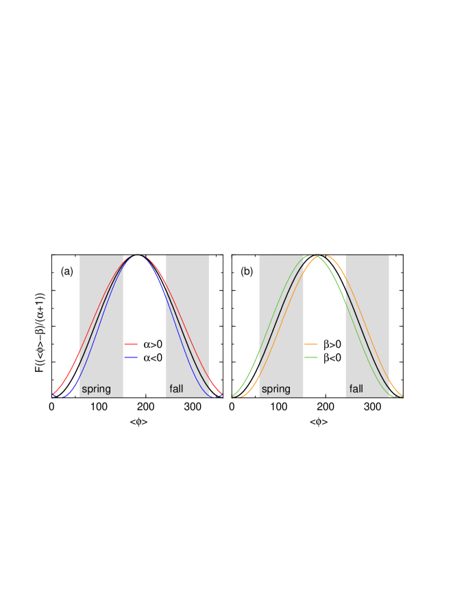
Figure 1: Idealized cycle of advantageous and disadvantageous phenological years as well as premature and delayed years. Illustration of the coefficients $\alpha$ and $\beta$ from Eq. (2). (a) Non-zero $\alpha$, which is the slope of the linear fit to $\phi-\langle\phi\rangle$ versus $\langle\phi\rangle$, constitutes a temporary change of the frequency. In the $\alpha>0$ case this leads to earlier phases in spring and later phases in fall. (b) Non-zero $\beta$, which is the intercept of the fit, constitutes a temporary phase shift, with overall earlier ($\beta<0$) or later ($\beta>0$) phases. Compare with Eq. (3). For illustration we use a shifted cosine as periodic function $F$.

We understand phenological processes to be triggered by an annual cycle that is a compound of all relevant climatological features. In general, such a cycle is unknown but we think of it as illustrated in Fig. 1. Once it passes a certain threshold, and its derivative has the right sign, such as positive for spring or negative for fall, a specific plant is activated and a phenological phase takes place, e.g. flowering in spring.

In B we show that the slope $\alpha$ is also associated with an increased or decreased cycle in such a way that the integral over an idealized annual cycle $C$ is approximately proportional to $\alpha$, as suggested by Fig. 1(a).

3 Data

The study region, North Rhine-Westphalia (NRW), is the most populous state of Germany ($\approx$ $18$ million residents in 2008; $34,070$ km² total area). Two types of landscapes can be found in NRW: the North German lowlands with an elevation just a few meters above sea level, and the North German low mountain range with elevations of up to $850$ m. The lowlands comprise the Rhine-Ruhr Area which is one of the largest metropolitan areas worldwide. These landscape features are also expressed by distinct types of climate. While in the lowlands the mean annual temperature is $10$ ^∘C with an annual mean precipitation of $620$ mm, in the mountainous regions the mean temperature is $5$ ^∘C and an annual mean precipitation of up to $1,500$ mm is common as measured between the years 1961-1990 [22].

Onset dates of numerous phenological phases have been collected in Germany by the German Weather Services (DWD) for the past decades. Observations are carried out two to three times in a week, which determines the temporal accuracy of the dataset. Since 1951 data for over $159$ phases has been observed at around $660$ stations in NRW. Due to incomplete datasets, especially before 1970, we have reduced the number of stations to those providing sufficient data for our purposes over the whole period from 1951 to 2006 (see C). As agricultural phases are strongly influenced by agricultural practices as well as breeding, and show a weaker relation to temperature changes [23], they were not considered in this study. Thus, we analyzed time series data of 17 meteorological and phenological stations in NRW for $75$ phases for the period of 1951-2006 (cf. Fig. 6). In order to investigate the effect of temperature on phenology, annual mean temperature records from the nearest climate station to each phenological station were further taken into account. Temperature records are based on observational data of the DWD and were partly interpolated [22]. In C we list the phenological phases and climatological stations.

4 Results

4.1 Fluctuations

In Figure 2 we show examples of $\varphi=\phi-\langle\phi\rangle$ versus $\langle\phi\rangle$, namely for the years 1960-1964, 1970, 1980, and 1990 at the station Dülmen. During winter, i.e. approx. $\langle\phi\rangle<50$ and $\langle\phi\rangle>300$, no phenological activity is recorded. While in 1960 [Fig. 2(a)] the phenological phases appear more or less as in average, in 1961 spring phases occurred prematurely. In 1962 all phases were delayed and in 1963 and 1964 the spring phases only.

In 1970 [Fig. 2(b)] spring phases occured late ($\varphi>0$) leading to a negative slope $\alpha$. In 1980 [Fig. 2(c)] less phases were recorded but on the basis of the available data it seems to have been a rather normal year. In 1990 [Fig. 2(d)] the early phases appear prematurely ($\varphi<0$) indicating good conditions in spring.

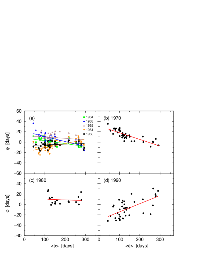
Figure 2: Examples of phase anomalies versus average phase in the case of Dülmen near Münster in North Rhine-Westphalia for the years (a) 1960-1964, (b) 1970, (c) 1980, and (d) 1990. The filled symbols represent the various phenological phases and the solid line is a linear fit through the data by least squares.

Next we want to address how strongly the phenological phases fluctuate. In order to quantify these fluctuations we use the Rayleigh measure [24, 21]:

$$\sigma_{\phi}=\sqrt{\langle\cos\phi\rangle^{2}+\langle\sin\phi\rangle^{2}}\,.$$ (4)

Here $\langle\cdot\rangle$ is the average over time, separately for each phenological plant. If $\phi$ is spread uniformly over the period then $\sigma_{\phi}$ is close to $0$ because the averages of the trigonometric functions are very small. If $\phi$ is fixed then $\sigma_{\phi}$ is $1$. Thus, values close to $0$ indicate large fluctuations and values close to $1$ small ones. We use this quantity since the standard deviation of an angle is not well defined. We would like to remark that $\sigma_{\phi}$ is independent of the regressions in Fig. 2.

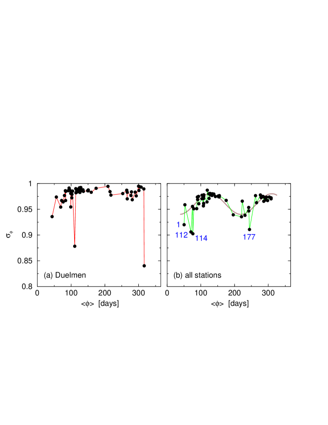
Figure 3: Fluctuations according to Eq. (4) of phenological phases (a) in the case of Dülmen in North Rhine-Westphalia and (b) for all stations. In both cases the average is over all available years. Small $\sigma_{\phi}$ correspond to large fluctuations. The solid line in the background of (b) illustrates the wavy pattern of the fluctuations (functional form $\propto\sin\langle\phi\rangle\cos\langle\phi\rangle$). The numbers indicate some phenological phases that are spread relatively strongly. 1: Hazel, Corylus Avellana: flowering; 112: European Alder, Alnus Glutinosa: flowering; 114: Cornel Cherry, Cornus Mas: flowering; and 177: Wild Brier, Rosa Canina: fruit ripening.

Figure 3 shows the spreading $\sigma_{\phi}$ versus the average phase $\langle\phi\rangle$. The result for the example from Fig. 2 is depicted in Fig. 3(a). Two phenological phases have small values of $\sigma_{\phi}$ and accordingly large spreading – which is due to measurement errors. Apart from that, most phases show $\sigma_{\phi}>0.95$ and only early phases exhibit larger fluctuations (smaller $\sigma_{\phi}$), compare with Fig. 2(a).

In contrast, the $\sigma_{\phi}$ obtained from all stations [Fig. 3(b)] look smoother and four phenological phases have rather small $\sigma_{\phi}$-values (large spreading). In general, a kind of wave pattern can be observed and is illustratively traced in Fig. 3(b): Spring phases exhibit larger fluctuations, early summer phases smaller ones, late summer phases again larger fluctuations, and fall phases again small ones. Calculating standard deviations, similar patterns have been found for $35$ plant phases and $29$ butterfly phases [15]. Assuming a wave (see Fig. 1 and B) those phases with small fluctuations coincide with large slopes (or small negative slopes) of an idealized phenological cycle.

Deviations from the curve could result from measurement inaccuracies, since for some phases (e.g. fruit ripening) the exact onset date is difficult to determine. Another reason could be that those phenological phases with small fluctuation are triggered by a sharp change while the others with larger fluctuations typically occur in seasons when the trigger is not as sharp. In other words, small deviations of the phenological cycle barely influence those phases that in average occur when the idealized cycle has a large slope. Contrariwise, small deviations of the phenological cycle do affect phases that in average occur when the idealized cycle has a small slope.

4.2 Phenological index

Systematically applying linear regressions to $\varphi=\phi-\langle\phi\rangle$ versus $\langle\phi\rangle$ of the example station Dülmen (solid lines in Fig. 2) we obtain a set of quantities in Fig. 4, plotted against the corresponding year. In Fig. 4(a) and (b) we show the two fit coefficients, namely the slope, $\alpha$, and the intercept, $\beta$, respectively. As pointed out in Sec. 2, the former indicates how advantageous a year is. We consider it as a phenological index (pheno-index). As can be seen, $\alpha$ fluctuates from year to year roughly in the range $-0.2<\alpha<0.2$.

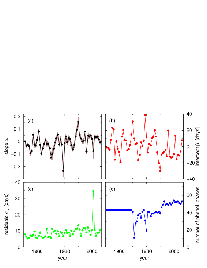
Figure 4: Values obtained for the phase anomaly fit Eq. (2) as illustrated in Fig. 2 for the years 1951-2006 (Dülmen). (a) slope $\alpha$ (pheno-index), (b) intercept $\beta$, (c) root mean square deviations from the fit $\sigma_{\varphi}$, and (d) number of phenological phases used for each year. The brownish area in the background of (a) corresponds to the standard error.

Two additional quantities of interest are depicted in Fig. 4(c) and (d). The root mean square deviations from the fit in Fig. 2, $\sigma_{\varphi}$, capture how uniform the annual cycle is or how homogeneously the phenological phases respond to the climate variations. We find that except from an outlier in the year 2001 (due to a measurement error) the residuals are stable with values around or below $10$ days. Remarkably, the outlier does not seem to affect much the values of $\alpha$ and $\beta$ in 2001. Figure 4(d) shows the number of phenological phases considered in the specific years; this is the same number of points appearing in the panels of Fig. 2. Somehow – for the example station – up to 1970 constantly 43 phases were recorded per year. In 1971 only 11 values are considered but still $\alpha$ and $\beta$ seem to have reasonable values, supporting the robustness of the approach.

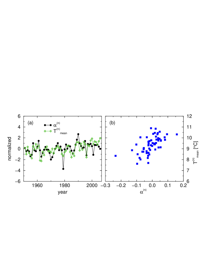
Figure 5: Correlations between pheno-index and annual mean temperature for the years 1951-2006 (Dülmen). (a) Comparison of annual mean temperature $T_{\rm mean}$ (open diamonds) and pheno-index $\alpha$ (filled circles). (b) Scatter plot of $T_{\rm mean}$ versus $\alpha$ for all years. For a better comparison, the records are normalized according to Eq. (5) and Eq. (6), respectively.

4.3 Correlations between phenological phases and temperature records

It is known that the temperature is an important climatological element influencing the phenological timing, in particular at springtime [3]. Next we want to inspect, how the pheno-index (slope $\alpha$) is related to the mean annual temperature $T_{\rm mean}$. Figure 5(a) shows both, $\alpha$ as well as $T_{\rm mean}$ measured at the closest climatological station, nearby Billerbeck, which is situated less than $20$ km from Dülmen. In order to compare the two quantities, we have normalized both records to zero average and unit standard deviation:

$$T_{\rm mean}^{\rm(n)}=(T_{\rm mean}-\langle T_{\rm mean}\rangle)/\sigma_{T}$$ (5)

as well as

$$\alpha^{\rm(n)}=(\alpha-\langle\alpha\rangle)/\sigma_{\alpha}\,.$$ (6)

We find a fair agreement between the course of both quantities. However, from 1999 onwards the normalized temperature values are above the normalized pheno-index. By definition, due to continuity reasons, $\alpha$ cannot systematically deviate from zero. Thus, further research is required to reveal if this is a systematic deviation or within the statistical fluctuations.

In Figure 5(b) the quantities $\alpha$ and $T_{\rm mean}$ are plotted against each other for each year. The correlation coefficient for this example is $0.60$, which is a satisfying result considering the noisy data of Fig. 2.

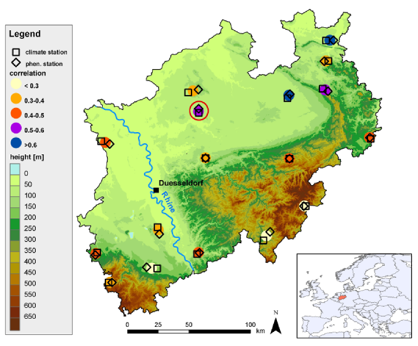
Figure 6: Area under investigation, North Rhine-Westphalia, and correlations between annual mean temperature and pheno-index. Since, in general, phenology (open diamonds) and temperature (open squares) are not measured at the same site, we identify the closest pairs and attribute the correlation value as a color-coded circle to the center between the two. The exemplary station Dülmen illustrated in the previous Figures is indicated by the red solid line circle.

Figure 6 exhibits the area under investigation, North Rhine-Westphalia. We identify for each phenological station the closest temperature station and calculate the correlation value between the pheno-index and the associated annual mean temperature record. The locations of the stations and the resulting correlation values are depicted in the map. The correlations vary between $0.28$ and $0.64$ and do not seem to show any systematic dependence on the position, indicating that micro-scale spatial climatological conditions may be dominating the pheno-index. In addition, the correlation value of $\alpha$ and $T_{\rm mean}$ does not significantly depend on the amount of phenological data of the stations.

For several reasons we do not expect much larger correlation coefficients for individual phenological stations. Certainly, the phenological phases are also influenced by other factors, in particular precipitation or sunshine duration. Precipitation has weak spatial correlations and could be responsible for micro-scale influences. Hence, including further information of this kind could improve the correlations. In addition, the spring phases are influenced by the beginning of the year and possibly by the end of the year before but certainly not by the end of the actual year. Thus, considering seasonal values or taking into account at least part of the previous year could also lead to stronger correlations. In addition, the fall phases are known to react in a less pronounced way to temperature [14, 4, 3] and could contribute to noise leading to reduced correlation values.

5 Discussion and Conclusions

In summary, we analyze phenological records, characterize the fluctuations of the phases, and introduce a phenological index. We find that the spring and late summer phases exhibit the largest fluctuations while the early summer and fall phases exhibit the smallest fluctuations. This may be related to the derivative of the annual cycle, such as of temperature. By plotting (for each individual station) the phase anomaly against the average of each phase and applying a linear regression through all phases, we obtain a measure for how advantageous a specific year was for the ensemble of flora at the corresponding site. The slope represents a temporary change of frequency and the intercept a temporary phase shift. In addition, we show that the slope of such a fit is approximately proportional to the integral over the idealized annual phenological cycle. The advantage of our approach is that it characterizes the multitude of climatological factors influencing the entire phenological ensemble considered. It smoothes the volatile phenological data to a combined index which helps to detect and quantify impacts on life and life cycles. It can be applied even when records are incomplete, something which can cause problems when phenological phases are considered individually. Generally, a similar index can also be calculated for the phenology of fauna, but this is a task we leave for future studies.

We compare the pheno-index with the annual mean temperature and find some agreement. The correlation value for various stations in the area of investigation varies between $0.28$ and $0.64$ whereas from this study we do not find any systematic dependence of the correlations on the location. We conclude that additional factors influence the pheno-index. The response of phenological phases to changes in temperature has been found to vary spatially, for example being stronger in more northerly latitudes [8]. Further, a more pronounced spring advance has been described for maritime western and central Europe compared to the continental east [17]. Temperature has been identified as the main driver of spring phases, followed by the photoperiod length. Other factors such as precipitation, nutrient availability and soil properties showed only minor effect in comparison to temperature [25]. Further research is needed in order to figure out how our approach relates to these previous findings.

Climate change induced shifts in phenology could disrupt the chain between pollinator and plants [26]. Phenological plant phases are key stages of plant development – changes in their timing might influence other species. Thus, alterations of phenological phases could disrupt interactions among species, e.g. within food webs [15], see also [27]. Evidence from various species indicate an insufficient rate of phenological adaptation concerning food webs to changing climatic conditions [28].

It has been found that correlations between air temperature and fall phases are less pronounced [14, 4, 3]. Thus, the application of the ideas of this work could lead to a better consideration of fall phases within phenological analysis. There is considerable interest on how phenology will be affected by climate change, particularly in the context of ecology or agriculture. The phenological index could be used as the basis of projections obtained from climate models to project the changes in phenology.

Appendix A Calculating the average phase $\langle\phi\rangle$

We want to calculate the average phase, $\langle\phi\rangle$, from a set of angles $\phi_{i}$. In order to account for the cyclicality of the phase, we do not simply average the phases, but consider the Euler relation, ${\rm e}^{{\rm i}\phi}=\cos\phi+{\rm i}\sin\phi$, average the sine and the cosine separately, and use the relation $\tan\theta=\frac{\sin\theta}{\cos\theta}$.

However, writing the inverse, $\langle\phi\rangle=\arctan\left(\frac{\langle\sin\phi\rangle}{\langle\cos\phi\rangle}\right)$, is not precise since the $\arctan$-function does not take into account the signs of numerator and denominator. Therefore, most programming languages provide the two argument function ${\rm atan2}$, which properly calculates the angle,

$$\langle\phi\rangle={\rm atan2}\left(\langle\sin\phi\rangle,\langle\cos\phi\rangle\right)\,.$$ (7)

Appendix B Relation between the pheno-index $\alpha$ and the anomaly of the phenological cycle

Although, the annual cycle of phenological advantage basically can have any periodic shape, we assume such a cycle has the form of a sine-wave (for simplicity we skip the indices $p$ and $t$):

$$C(\phi)=A\sin(\phi+\lambda)+B\,,$$ (8)

where $A$ is the amplitude, $\phi=\nu t$ the phase (frequency $\nu$), $\lambda$ the phase shift, and $B$ an offset. We would like to remark that it would be more meaningful to express $\phi$ as a function of $C$, since the annual cycle triggers the phenological phases. Due to climate fluctuation, the cycle $C$ deviates from the average annual cycle within a year as well as from year to year. Since such an idealized cycle is unknown, we study the phenological signals.

Here we show that the slope $\alpha$ is associated with an increased or decreased cycle in such a way that the integral over $C$ is approximately proportional to $\alpha$, as suggested by Fig. 1(a).

The integral over one period of the average annual cycle vanishes when we drop the offset

$$\int_{-\pi}^{\pi}\!\left[A\sin(\langle\phi\rangle+\langle\lambda\rangle)\right]{\rm d}\langle\phi\rangle=0\,.$$ (9)

The quantities $\phi$ and $\lambda$ are spread around $\langle\phi\rangle$ and $\langle\lambda\rangle$, respectively (assuming $A={\rm const.}$), and are in general different from the averages. Using Eq. (3) in (8) we express the integral over $C$ as

$$\int_{-\pi}^{\pi}\!\left[A\sin(\langle\phi\rangle(\alpha+1)+\beta+\lambda)\rangle\right]{\rm d}\langle\phi\rangle$$ (10)

$$= \left[-\frac{A}{(\alpha+1)}\cos(\langle\phi\rangle(\alpha+1)+\beta+\lambda)\right]_{-\pi}^{\pi}$$

$$= -\frac{A}{(\alpha+1)}\left[\cos(\pi(\alpha+1)+\beta+\lambda)-\cos(-\pi(\alpha+1)+\beta+\lambda)\right]$$

$$= -\frac{A}{(\alpha+1)}[\cos(\pi(\alpha+1))\cos(\beta+\lambda)-\sin(\pi(\alpha+1))\sin(\beta+\lambda)$$

$${}-\left(\cos(-\pi(\alpha+1))\cos(\beta+\lambda)-\sin(-\pi(\alpha+1))\sin(\beta+\lambda)\right)]$$

$$= \frac{2A}{(\alpha+1)}\sin(\pi(\alpha+1))\sin(\beta+\lambda)$$

Since $\beta+\lambda\approx-\pi/2$ (in order to match the seasons within the calendar year) the second term is $\sin(\beta+\lambda)\approx-1$. For $\alpha$ close to $0$, the first term goes like $-\pi\alpha$ and assuming $\alpha+1\approx 1$ one obtains

$$\int_{-\pi}^{\pi}\!\left[A\sin(\langle\phi\rangle(\alpha+1)+\beta+\lambda)\rangle\right]{\rm d}\langle\phi\rangle{} {}\approx{} {}2\pi A\alpha$$ (11)

$${}\sim{} {}\alpha\,.$$ (12)

Therefore, we conclude that $\alpha$, as the regression slope to $\phi-\langle\phi\rangle$ versus $\langle\phi\rangle$, is a measure for the anomaly of the phenological cycle with respect to early spring phases and late fall phases and vice versa. However, the unchanged maximum in Fig. 1(a) is not very realistic. Having in mind a temperature change, one would expect an overall vertical shift of the cycle and accordingly rather an anomaly reflected in the offset $B$. Nevertheless, since there are few phenological phases in winter (where no events are measured) and since the analysis is performed statistically, $\alpha$ can still be considered as a measure for the in- or decrease of the phenological cycle.

Appendix C Details on the phenological data

The observational program of wild plants includes the following codes: 1-20, 64-74, 112-135, 175-178, 213-228, which are listed at http://www.dwd.de $>$ Climate + Environment $>$ Phenology $>$ Observation programme $>$ Wild plants. In order to have sufficient statistics, we filter the phenology data according to the following criteria: (i) phenological phases with at least $3$ entries for one station, (ii) years with at least $3$ pairs of $\langle\phi\rangle$, $\varphi$, and (iii) stations with at least $30$ years of data, whereas the presence of the years 1951 and 2006 is required. The phenological and associated temperature stations are listed in Tab. 1. Daily temperature records have been averaged to annual resolution. Missing temperature data has been interpolated [22].

Table 1: Phenological and associated temperature stations

phenological stations		climate stations
ID	location	PIK-ID	location
52334110	Kevelaer, Kleve	19183	Weeze-Hees
53331130	Zülpich, Euskirchen	19006	Euskirchen
53341120	Frechen, Erftkreis	19107	Pulheim-Brauweiler
53371170	Hennef, Rhein-Sieg-Kreis	19113	Hennef
54110000	Aachen (DWD), kreisfreie Stadt Aachen	19004	Aachen
54352120	Imgenbroich, Aachen	19119	Monschau
55342130	Billerbeck, Coesfeld	19175	Coesfeld
55344110	Dülmen, Coesfeld	19177	Billerbeck
57331490	Heidenoldendorf, Lippe	20339	Lage, Kr.Lippe-Hoerste
57359110	Exter, Herford	15208	Vlotho-Valdorf
57391110	Minden, Minden-Lübbecke	15182	Minden-Hahlen
57412130	Bühne, Höxter	20031	Borgenb
57421110	Gütersloh, Gütersloh	20022	Guetersl
58326170	Warstein, Hochsauerlandkreis	20259	Warstein
58397360	Obernetphen, Soest	20013	Siegen
58422410	Wunderthausen, Siegen-Wittgenstein	20291	Berleburg, Bad-Wunderthausen
59230000	Witten-Stockum, Ennepe-Ruhr-Kreis	19221	Witten-Stockum

References

References

- [1] I. L. Hudson, Interdisciplinary approaches: towards new statistical methods for phenological studies, Climatic Change 100 (1) (2010) 143–171.
- [2] P. Bissolli, G. Müller-Westermeier, C. Polte-Rudolf, Aufbereitung und Darstellung phänologischer Daten, Promet 33 (1/2) (2007) 14–19.
- [3] G. R. Walther, E. Post, P. Convey, A. Menzel, C. Parmesan, T. J. C. Beebee, J. M. Fromentin, O. Hoegh-Guldberg, F. Bairlein, Ecological responses to recent climate change, Nature 416 (6879) (2002) 389–395.
- [4] A. Menzel, T. H. Sparks, N. Estrella, E. Koch, A. Aasa, R. Ahas, K. Alm-Kubler, P. Bissolli, O. Braslavska, A. Briede, F. M. Chmielewski, Z. Crepinsek, Y. Curnel, A. Dahl, C. Defila, A. Donnelly, Y. Filella, K. Jatcza, F. Mage, A. Mestre, O. Nordli, J. Penuelas, P. Pirinen, V. Remisova, H. Scheifinger, M. Striz, A. Susnik, A. J. H. van Vliet, F. E. Wielgolaski, S. Zach, A. Zust, European phenological response to climate change matches the warming pattern, Global Change Biology 12 (10) (2006) 1969–1976.
- [5] C. Rosenzweig, G. Casassa, D. J. Karoly, A. Imeson, C. Liu, A. Menzel, S. Rawlins, T. L. Root, B. Seguin, P. Tryjanowski, Assessment of observed changes and responses in natural and managed systems, in: M. L. Parry, O. F. Canziani, J. P. Palutikof, P. J. van der Linden, C. E. Hanson (Eds.), Climate Change 2007: Impacts, Adaptation and Vulnerability. Contribution of Working Group II to the Fourth Assessment Report of the Intergovernmental Panel on Climate Change, Cambridge University Press, Cambridge, UK, 2007, pp. 79–131.
- [6] A. Menzel, N. Estrella, A. Testka, Temperature response rates from long-term phenological records, Climate Research 30 (1) (2005) 21–28.
- [7] W. Schröder, G. Schmidt, J. Hasenclever, Geostatistical analysis of data on air temperature and plant phenology from Baden-Wurttemberg (Germany) as a basis for regional scaled models of climate change, Environmental Monitoring and Assessment 120 (1-3) (2006) 27–43.
- [8] N. Estrella, T. H. Sparks, A. Menzel, Effects of temperature, phase type and timing, location, and human density on plant phenological responses in Europe, Climate Research 39 (3) (2009) 235–248.
- [9] Y. Aono, K. Kazui, Phenological data series of cherry tree flowering in Kyoto, Japan, and its application to reconstruction of springtime temperatures since the 9th century, International Journal of Climatology 28 (7) (2008) 905–914.
- [10] R. B. Primack, H. Higuchi, A. J. Miller-Rushing, The impact of climate change on cherry trees and other species in Japan, Biological Conservation 142 (9) (2009) 1943–1949.
- [11] V. Dose, A. Menzel, Bayesian correlation between temperature and blossom onset data, Global Change Biology 12 (2006) 1451–1459.
- [12] C. Schleip, T. H. Sparks, N. Estrella, A. Menzel, Spatial variation in onset dates and trends in phenology across Europe, Climate Research 39 (3) (2009) 249–260.
- [13] T. H. Sparks, B. Jaroszewicz, M. Krawczyk, P. Tryjanowski, Advancing phenology in Europe’s last lowland primeval forest: non-linear temperature response, Climate Research 39 (3) (2009) 221–226.
- [14] M. S. Abu-Asab, P. M. Peterson, S. G. Shetler, S. S. Orli, Earlier plant flowering in spring as a response to global warming in the Washington, DC, area, Biodiversity and Conservation 10 (4) (2001) 597–612.
- [15] A. Menzel, T. H. Sparks, N. Estrella, D. B. Roy, Altered geographic and temporal variability in phenology in response to climate change, Global Ecology and Biogeography 15 (5) (2006) 498–504.
- [16] P. Tryjanowski, M. Panek, T. Sparks, Phenological response of plants to temperature varies at the same latitude: case study of dog violet and horse chestnut in England and Poland, Climate Research 32 (1) (2006) 89–93.
- [17] R. Ahas, J. Jaagus, A. Aasa, The phenological calendar of Estonia and its correlation with mean air temperature, International Journal of Biometeorology 44 (4) (2000) 159–166.
- [18] F.-M. Chmielewski, A. Müller, W. Küchler, Mögliche Auswirkungen klimatischer Veränderungen auf die Vegetationsentwicklung in Sachsen, Tech. rep., Eigenverlag HU Berlin (2004).
- [19] P. Bissolli, G. Müller-Westermeier, E. Dittmann, V. Remisova, O. Braslavska, P. Stastny, 50-year time series of phenological phases in Germany and Slovakia: a statistical comparison, Meteorologische Zeitschrift 14 (2) (2005) 173–182.
- [20] A. H. Fitter, R. S. R. Fitter, Rapid changes in flowering time in British plants, Science 296 (5573) (2002) 1689–1691.
- [21] M. H. Trauth, MATLAB® Recipes for Earth Sciences, Springer Berlin Heidelberg, Berlin, Heidelberg, 2010. doi:10.1007/978-3-642-12762-5.
- [22] H. Österle, P.-C. Werner, F.-W. Gerstengarbe, Qualitätsprüfung, Ergänzung und Homogenisierung der täglichen Datenreihen in Deutschland, 1951-2003: ein neuer Datensatz, 7. Deutsche Klimatagung, Klimatrends: Vergangenheit und Zukunft, 9.- 11. Oktober 2006, München, http://www.meteo.physik.uni-muenchen.de/dkt/poster.html (2006).
- [23] A. Menzel, J. von Vopelius, N. Estrella, C. Schleip, V. Dose, Farmers’ annual activities are not tracking the speed of climate change, Climate Research 32 (3) (2006) 201–207.
- [24] M. G. Rosenblum, A. S. Pikovsky, C. Schäfer, P. A. Tass, J. Kurths, Neuro-Informatics and Neural Modelling (Handbook of Biological Physics), Vol. 4, Elsevier Science B.V., North-Holland, Amsterdam, 2001, Ch. 9, pp. 279–322.
- [25] F. W. Badeck, A. Bondeau, K. Bottcher, D. Doktor, W. Lucht, J. Schaber, S. Sitch, Responses of spring phenology to climate change, New Phytologist 162 (2) (2004) 295–309.
- [26] J. Memmott, P. G. Craze, N. M. Waser, M. V. Price, Global warming and the disruption of plant-pollinator interactions, Ecology Letters 10 (8) (2007) 710–717.
- [27] J. Camacho, R. Guimera, L. A. N. Amaral, Robust patterns in food web structure, Physical Review Letters 88 (22) (2002) 228102.
- [28] M. E. Visser, C. Both, Shifts in phenology due to global climate change: the need for a yardstick, Proceedings of the Royal Society B – Biological Sciences 272 (1581) (2005) 2561–2569.