The string of variable density: further results

Abstract

We analyze the problem of calculating the solutions and the spectrum of a string with arbitrary density and fixed ends. We build a perturbative scheme which uses a basis of WKB-type functions and obtain explicit expressions for the eigenvalues and eigenfunctions of the string. Using this approach we show that it is possible to derive the asymptotic (high energy) behavior of the string, obtaining explicit expressions for the first three coefficients (the first two can also be obtained with the WKB method). Finally using an iterative approach we also obtain analytical expressions for the low energy behavior of the eigenvalues and eigenfunctions of a string with rapidly oscillating density, recovering (in a simpler way) results in the literature.

1 Introduction

In this paper we consider the problem of calculating the normal modes of a string with arbitrary density and finite length. In a recent paper, ref. [1], we have considered the same problem, and we have proved the following results: first, that it is possible to apply iterative techniques and obtain increasingly refined approximations to selected normal modes of the string, starting from a particular ansatz; second, that it is possible to use a perturbative approach, corresponding to an expansion in the small inhomogeneities of the string, and thus prove that to second order in this expansion the perturbative results reproduce the asymptotic high energy behavior obtained with the WKB method. This result, which is not a–priori obvious, depends crucially on the dimensionality of the problem, since in one dimension the perturbative contributions depending on off-diagonal terms are not neglegible in the limit of asymptotically large energies (as it seems to be the case in more than one dimension).

The purpose of this work is twofold: on one hand, to devise an alternative perturbative approach, which is applicable to strings of arbitrary density (including highly inhomoegeneous cases); on the other hand to show that the iterative theorems of ref. [1], may be used to obtain extremely precise (numerical and analytical) results when applied to non–trivial problems.

The paper is organized as follows: in Section 2 we review the density perturbation theory (DPT) of ref. [1]; in Section 3 we devise an alternative perturbative method which uses a basis built out of WKB solutions and derive explicit analytical expressions for the first three coefficients of the asymptotic expansion for the energy: while the first two coefficients were already known (they can be obtained with the standard WKB method), the third coefficient is new (to the best of our knowledge) and it takes the form of an infinite series of divergent series (each of which can be Borel resummed); in Section 4 we describe a modified version of this alternative perturbative method, which uses WKB-type solutions, corresponding to non–physical densities and which may provide a better description of selected modes of the string; in Section 5 we briefly review the iterative theorems of ref. [1]; in Section 6 we discuss several applications of the methods of previous sections: in particular we test with high precision the analytical formula for the third asymptotic coefficient, and we apply the iterative methods to obtain the asymptotic behavior of the low energy spectrum of a string with highly oscillating density, thus reproducing results obtained in the literature [2]; finally in Section 8 we draw our conclusions.

2 Density perturbation theory

The starting point of our discussion is the Helmholtz equation

$$-\frac{d^{2}\Psi_{n}(x)}{dx^{2}}=E_{n}\rho(x)\Psi_{n}(x)$$ (1)

which describes the vibrations of a string of density $\rho(x)$. We assume that the string is centered in the origin and that it has a length $2L$. The solutions $\Psi_{n}(x)$ are orthogonal [3]

$$\int_{-L}^{+L}\Psi_{n}(x)\Psi_{m}(x)\rho(x)dx=\delta_{mn}$$ (2)

and obey specific boundary conditions at the border. In this paper we consider only Dirichlet boundary conditions, i.e. $\Psi_{n}(\pm L)=0$.

Equation (1) can be cast into a more convenient form by introducing the functions $\Phi_{n}(x)\equiv\sqrt{\rho(x)}\Psi_{n}(x)$ and writing it as

$$\frac{1}{\sqrt{\rho(x)}}\left[-\frac{d^{2}}{dx^{2}}\right]\frac{1}{\sqrt{\rho(x)}}\ \Phi_{n}(x)=E_{n}\Phi_{n}(x)\ .$$ (3)

The operator $\hat{O}\equiv\frac{1}{\sqrt{\rho(x)}}\left[-\frac{d^{2}}{dx^{2}}\right]\frac{1}{\sqrt{\rho(x)}}$ has a manifestly hermitian form and its eigenvalues and eigenfunctions are directly related to those of eq. (1). The results of refs.[1, 4, 5] are obtained using this symmetrized form for the differential operator of the inhomogeneous Helmholtz equation.

We now assume that the density $\rho(x)$ of the string may be expressed as

$$\rho(x)=\rho_{0}\left(1+\eta\ \delta\rho(x)\right)\ ,$$ (4)

where $\left|\delta\rho(x)\right|\ll 1$ and $\rho(x)>0$ for $x\in(-L,L)$. $\eta$ is a non-physical parameter used to allow power-counting (eventually this parameter is set to one). Under these assumptions $\delta\rho$ represents a perturbation and therefore one may use perturbation theory.

We expand the operator $\hat{O}$ in a power series

$$\hat{O}=\sum_{n=0}^{\infty}\hat{O}_{n}\eta^{n}\ .$$ (5)

where [1, 4]

$$\rho_{0}\hat{O}_{0} = -\frac{d^{2}}{dx^{2}}\ ,$$ (6)

$$\rho_{0}\hat{O}_{1} = -\frac{1}{2}\left[\delta\rho\left(-\frac{d^{2}}{dx^{2}}\right)+\left(-\frac{d^{2}}{dx^{2}}\right)\delta\rho\right]\ ,$$ (7)

$$\rho_{0}\hat{O}_{2} = \frac{1}{8}\left[2\delta\rho\left(-\frac{d^{2}}{dx^{2}}\right)\delta\rho+3\delta\rho^{2}\left(-\frac{d^{2}}{dx^{2}}\right)+3\left(-\frac{d^{2}}{dx^{2}}\right)\delta\rho^{2}\right]\ ,$$ (8)

$$\rho_{0}\hat{O}_{3} = -\frac{3}{16}\left[\delta\rho^{2}\left(-\frac{d^{2}}{dx^{2}}\right)\delta\rho+\delta\rho\left(-\frac{d^{2}}{dx^{2}}\right)\delta\rho^{2}\right]$$ (9)

$$- \frac{5}{16}\left[\delta\rho^{3}\left(-\frac{d^{2}}{dx^{2}}\right)+\left(-\frac{d^{2}}{dx^{2}}\right)\delta\rho^{3}\right]\ .$$

$$\dots$$

As standard in perturbation theory we assume that the eigenvalues and eigenfunctions of eq. (3) can be expressed as power series of the perturbation density $\delta\rho$, i.e. that

$$E_{n}=\sum_{k=0}^{\infty}E_{n}^{(k)}\eta^{k}\$$ (10)

and

$$\Phi_{n}(x)=\sum_{k=0}^{\infty}\Phi_{n}^{(k)}(x)\eta^{k}\ .$$ (11)

Clearly $E_{n}^{(0)}$ and $\Phi_{n}^{(0)}(x)$ are the energies and the solutions for a uniform string of density $\rho_{0}$; we also call $\epsilon_{n}$ the energies of a uniform string of unit density and use the Dirac bra-ket notation to represent the modes.

Readers familiar with perturbation theory for stationary states in Quantum Mechanics, i.e. with the Rayleigh-Schrödinger perturbation theory (RSPT), may easily spot the similarities and the differences between the typical implementation of RSPT and the present case: the approach that we follow here is the standard one used in the treatment of time independent perturbations in quantum mechanical problems, although in a typical quantum mechanical problem the Hamiltonian is polynomial in the coupling (most likely a linear function of $g$). In the present case the perturbation is the density $\delta\rho(x)$ and it appears in a non-polynomial form in the symmetrized operator of eq.(4).

As a result, at a given order in $\eta$ there will be contributions stemming from the operators of different orders $\hat{O}_{n}$ allowed to contribute to that given order and therefore there will be a proliferation of terms as higher orders in $\eta$ are considered.

The first few corrections to the energies of the string have been worked out explicitly in ref. [1, 4] and read:

$$\rho_{0}\ E_{n}^{(0)} = \epsilon_{n}$$ (12)

$$\rho_{0}\ E_{n}^{(1)} = -\epsilon_{n}\langle n|\delta\rho|n\rangle$$ (13)

$$\rho_{0}\ E_{n}^{(2)} = \epsilon_{n}\langle n|\delta\rho|n\rangle^{2}+\epsilon_{n}^{2}\sum_{k\neq n}\frac{\langle n|\delta\rho|k\rangle^{2}}{\epsilon_{n}-\epsilon_{k}}$$ (14)

$$\rho_{0}\ E_{n}^{(3)} = -\epsilon_{n}\langle n|\delta\rho|n\rangle^{3}+\epsilon_{n}^{3}\langle n|\delta\rho|n\rangle\sum_{k\neq n}\frac{\langle n|\delta\rho|k\rangle^{2}}{\omega_{nk}^{2}}$$ (15)

$$- 3\epsilon_{n}^{2}\langle n|\delta\rho|n\rangle\sum_{k\neq n}\frac{\langle n|\delta\rho|k\rangle^{2}}{\omega_{nk}}$$

$$- \epsilon_{n}^{3}\sum_{k\neq n}\sum_{m\neq n}\frac{\langle n|\delta\rho|k\rangle\langle k|\delta\rho|m\rangle\langle m|\delta\rho|n\rangle}{\omega_{nk}\omega_{nm}}\ ,$$

where $\epsilon_{n}=n^{2}\pi^{2}/\rho_{0}$ and $\omega_{nk}\equiv\epsilon_{n}-\epsilon_{k}$.

Here the reader will easily recognize that the direct terms at each order, i.e. the terms involving matrix elements of $\delta\rho$ between the same states, appear to originate from a geometric series. These terms may be resummed into

$$E_{n}|^{(direct)}\approx\frac{\epsilon_{n}}{\langle n|\rho(x)|n\rangle}$$ (16)

which for $n\rightarrow\infty$ would lead to an asymptotic behaviour

$$\lim_{n\rightarrow\infty}E_{n}|^{(direct)}\approx\frac{\epsilon_{n}}{\int_{-L}^{+L}\rho(x)dx}\ .$$ (17)

In two dimensions, when $\rho(x)$ is the density obtained from a conformal map which transforms an arbitrary domain into a square, the denominator of this equation provides the area of original domain, thus leading to a alternative derivation of Weyl’s law, based on perturbation theory [5]. The validity of this result however requires that the direct terms dominate asymptotically the terms in the perturbation series which mix the different states. A specific case discussed in ref. [4] concerning the small deformations of a square, has been proved to fulfill this requirement to second order.

In one dimension the situation is different: for this case we have proved in ref. [1] that for $n\rightarrow\infty$

$$\rho_{0}\ \frac{E_{n}^{(2)}}{\epsilon_{n}} \approx \frac{1}{4}\langle\sigma^{2}\rangle+\frac{3}{4}\langle\sigma\rangle^{2}\ .$$ (18)

This equation is consistent with the asymptotic behaviour which is obtained using the WKB method [3],

$$E_{n}\approx\frac{\epsilon_{n}}{\langle\sqrt{\rho(x)}\rangle^{2}}\ ,$$ (19)

where $\langle\sqrt{\rho}\rangle\equiv\frac{1}{2L}\int_{-L}^{L}\sqrt{\rho(x)}dx$.

One could regard this equation as Weyl’s law for an inhomogeneous string.

We will now apply the variational principle to obtain useful upper bounds to the energy of the fundamental mode of a string with arbitrary density. First we observe that the spectrum of the hermitian operator $\hat{O}$ corresponding to this string is positive and bounded from below; if we let $\Psi(x)$ be an arbitrary function obeying Dirichlet boundary conditions at the ends of the string then the expectation value of $\hat{O}$ in this state is an upper bound to the exact energy of the fundamental mode:

$$\langle\hat{O}\rangle_{\Psi}\geq E_{1}\ .$$ (20)

The proof of this statement is straightforward once $\Psi(x)$ is expanded in the basis formed by the eigenstates of $\hat{O}$.

Working to lowest order we use the fundamental mode of a uniform string of density $\rho_{0}$ as a variational ansatz

$$\Psi(x)=\sqrt{\frac{1}{L}}\sin\left[\pi\frac{(x+L)}{2L}\right]$$ (21)

and obtain the bound

$$\langle\hat{O}\rangle_{\Psi} = -\int_{-L}^{+L}\frac{\pi^{2}\cos^{2}\left(\frac{\pi x}{2L}\right)}{4L^{3}\rho(x)}dx+\int_{-L}^{+L}\frac{\pi\sin\left(\frac{\pi x}{2L}\right)\cos\left(\frac{\pi x}{2L}\right)\rho^{\prime}(x)}{2L^{2}\rho(x)^{2}}dx$$ (22)

$$- \int_{-L}^{+L}\ \frac{\cos^{2}\left(\frac{\pi x}{2L}\right)\rho^{\prime\prime}(x)}{2L\rho(x)^{2}}dx+\int_{-L}^{+L}\ \frac{3\cos^{2}\left(\frac{\pi x}{2L}\right)\rho^{\prime}(x)^{2}}{4L\rho(x)^{3}}dx\geq E_{1}\ .$$

This bound is expected to be useful only for slightly inhomogeneous strings.

3 WKB perturbation theory

We now describe a different approach to the problem of a string of variable density. This approach has been first used by Lindblom and Robiscoe in ref. [6], where the inhomogeneous Helmholtz equation was cast in the form of an equivalent Schrödinger equation on the finite domain and approximate expressions for the eigenvalues of eq. (1) were obtained.

The path that we follow here is similar to that of ref. [6], although our primary interest lies in the development of a perturbative expansion for the eigenvalues and eigenfunctions of eq. (1).

We first define the functions

$$\phi_{n}(x)\equiv\sqrt{\frac{2}{\sigma(L)}}\ \rho(x)^{1/4}\ \sin\left[n\pi\frac{\sigma(x)}{\sigma(L)}\right]\ \ \ ,\ \ \ n=1,2,\dots$$ (23)

where

$$\sigma(x)\equiv\int_{-L}^{x}\sqrt{\rho(y)}dy\ .$$ (24)

After making the change of variable $u=\sigma(x)/\sigma(L)$ it is straightforward to see that that these functions are orthonormal on $[-L,L]$, i.e. that

$$\int_{-L}^{+L}\phi_{n}(x)\phi_{m}(x)dx=\delta_{nm}\ .$$ (25)

This should not be a surprise since the change of variable relates these functions to the eigenfunctions of a uniform string. Moreover, the $\phi_{n}(x)$ are closely related to the WKB functions (see for example eq.(10.1.31) of Bender and Orszag, ref. [3], at pag.490).

Let us now consider the action of the symmetrized differential operator $\hat{O}$ which has been introduced in the previous section on any of the functions given above; with elementary algebra we see that

$$\hat{O}\phi_{n}(x)=\left[\frac{n^{2}\pi^{2}}{\sigma(L)^{2}}+\frac{4\rho(x)\rho^{\prime\prime}(x)-5\rho^{\prime}(x)^{2}}{16\rho(x)^{3}}\right]\phi_{n}(x)\ .$$ (26)

For the highly excited states ($n\gg 1$) the second term in the parenthesis is neglegible with respect to the first and the $\phi_{n}(x)$ become increasingly good approximations to the exact eigenfunctions of $\hat{O}$, as usual in the WKB approximation.

The $\phi_{n}$ are eigenfunctions of the hermitian operator $\hat{Q}$:

$$\hat{Q}\phi_{n}(x)\equiv\left[\hat{O}-\frac{4\rho(x)\rho^{\prime\prime}(x)-5\rho^{\prime}(x)^{2}}{16\rho(x)^{3}}\right]\phi_{n}(x)=\frac{n^{2}\pi^{2}}{\sigma(L)^{2}}\phi_{n}(x)\ ,$$ (27)

whose eigenvalues coincide with the leading WKB expression for the eigenvalues of eq. (1).

In special cases the $\phi_{n}(x)$ provide the exact solutions to the full problem: this happens when the density is such that

$$\frac{4\rho(x)\rho^{\prime\prime}(x)-5\rho^{\prime}(x)^{2}}{16\rho(x)^{3}}=\kappa\ ,$$ (28)

where $\kappa$ is a constant.

The general solution to this ordinary differential equation has the form

$$\rho(x)=\frac{256c_{1}^{2}}{\left(c_{1}^{2}\left(c_{2}+x\right){}^{2}-256\kappa\right){}^{2}}\ ,$$ (29)

where $c_{1}$ and $c_{2}$ are integration constants; the density discussed by Borg in [7] is a special case corresponding to

$$c_{1}=\frac{16\alpha^{2}}{1+\alpha}\ \ ,\ \ c_{2} = L+\frac{1}{\alpha}\ \ ,\ \ \kappa=0\ .$$ (30)

With the purpose of implementing a perturbative expansion we define the operator

$$\hat{O}_{\eta}\equiv\hat{Q}+\eta\ \frac{4\rho(x)\rho^{\prime\prime}(x)-5\rho^{\prime}(x)^{2}}{16\rho(x)^{3}}\equiv\hat{Q}+\eta V(\sigma(x))\ ,$$ (31)

where $\eta$ once again is a non-physical parameter used for power counting ($\hat{O}_{1}=\hat{O}$) and $V(\sigma(x))$ is a potential defined in terms of the density. We assume that the eigenvalues and eigenfunctions of $\hat{O}$ can be expressed as power series in $\eta$, as done before in eqs. (10) and (11) for the DPT. Unlike for the DPT we notice that here the density $\rho(x)$ is not bound to be a perturbation and that $\hat{O}_{\eta}$ is an operator which depends linearly on $\eta$. Because of this last property the corrections for the energies of the string in this approach have a simpler form than in those in the DPT.

We write explicitly the first few terms:

$$E_{n}^{(0)} = \frac{n^{2}\pi^{2}}{\sigma(L)^{2}}\ ,$$ (32)

$$E_{n}^{(1)} = \langle n|V|n\rangle\ ,$$ (33)

$$E_{n}^{(2)} = \frac{\sigma(L)^{2}}{\pi^{2}}\sum_{k\neq n}\frac{|\langle n|V|k\rangle|^{2}}{(n^{2}-k^{2})}$$ (34)

$$E_{n}^{(3)} = \frac{\sigma(L)^{4}}{\pi^{4}}\sum_{k\neq n}\sum_{l\neq n}\frac{\langle n|V|k\rangle\langle k|V|l\rangle\langle l|V|n\rangle}{(n^{2}-k^{2})(n^{2}-l^{2})}$$ (35)

$$- \frac{\sigma(L)^{4}}{\pi^{4}}\langle n|V|n\rangle\sum_{k\neq n}\frac{\langle n|V|k\rangle^{2}}{(n^{2}-k^{2})^{2}}$$

$$\dots = \dots$$

Using eq. (31) we may cast these expressions directly in terms of the operator $\hat{O}$, taking into account that $\langle n|\hat{O}|k\rangle=\langle n|V|k\rangle$ for $k\neq n$. Notice that the second order correction to the energy of the fundamental mode is always negative as in the standard RSPT.

Similarly for the eigenfunctions we may write

$$\phi_{n}^{(0)}(x) = \phi_{n}(x)$$ (36)

$$\phi_{n}^{(1)}(x) = \frac{\sigma(L)^{2}}{\pi^{2}}\sum_{k\neq n}\frac{\langle k|V|n\rangle}{n^{2}-k^{2}}\phi_{k}(x)$$ (37)

$$\phi_{n}^{(2)}(x) = \frac{\sigma(L)^{4}}{\pi^{4}}\sum_{k\neq n}\sum_{j\neq n}\frac{\langle k|V|j\rangle\langle j|V|n\rangle}{(n^{2}-k^{2})(n^{2}-j^{2})}\phi_{k}(x)$$ (38)

$$- \frac{\sigma(L)^{4}}{\pi^{4}}\langle n|V|n\rangle\sum_{k\neq n}\frac{\langle k|V|n\rangle}{(n^{2}-k^{2})^{2}}\phi_{k}(x)$$

$$\phi_{n}^{(3)}(x) = -\frac{\sigma(L)^{6}}{\pi^{6}}\langle n|V|n\rangle\sum_{k\neq n}\sum_{j\neq n}\frac{\langle k|V|j\rangle\langle j|V|n\rangle}{(n^{2}-k^{2})^{2}}\phi_{k}(x)$$ (39)

$$+ \frac{\sigma(L)^{6}}{\pi^{6}}\langle n|V|n\rangle^{2}\sum_{k\neq n}\frac{\langle k|V|n\rangle}{(n^{2}-k^{2})^{3}}\phi_{k}(x)$$

$$+ \frac{\sigma(L)^{6}}{\pi^{6}}\sum_{k\neq n}\sum_{j\neq n}\sum_{l\neq n}\frac{\langle n|V|l\rangle\langle l|V|n\rangle\langle k|V|j\rangle}{(n^{2}-k^{2})(n^{2}-j^{2})(n^{2}-l^{2})}\phi_{k}(x)$$

$$- \frac{\sigma(L)^{6}}{\pi^{6}}\langle n|V|n\rangle\sum_{k\neq n}\sum_{l\neq n}\frac{\langle n|V|l\rangle\langle l|V|n\rangle}{(n^{2}-k^{2})^{2}(n^{2}-l^{2})}\phi_{k}(x)$$

$$- \frac{\sigma(L)^{6}}{\pi^{6}}\sum_{k\neq n}\sum_{j\neq n}\frac{\langle n|V|l\rangle\langle j|V|n\rangle^{2}}{(n^{2}-k^{2})^{2}(n^{2}-j^{2})}\phi_{k}(x)$$

$$\dots = \dots$$

The expressions that we have written above are equivalent to those found in ref. [6]; in particular eq.(2) of that paper is just the energy of a string calculated to first order in this scheme.

We will now derive asymptotic expressions for the energies of a string of variable density using these perturbative formulas and compare them with the asymptotic formulas obtained by Lindblom and Robiscoe.

As we have already mentioned, eq. (32) is just the leading term for the energy of an inhomogeneous string obtained with the standard WKB method [3]. The differences with the WKB results appear at first order, in $E_{n}^{(1)}$; with a simple change of variable we may cast eq. (33) as

$$E_{n}^{(1)}=\frac{2}{\sigma(L)}\ \int_{0}^{\sigma(L)}\sin^{2}\left[n\pi\frac{\sigma}{\sigma(L)}\right]V(\sigma(x))d\sigma\ .$$ (40)

Eq.(2) of ref. [6] contains this expression.

We may now use the results of A to write $E_{n}^{(1)}$ in the equivalent form

$$E_{n}^{(1)}=\langle V\rangle-\sum_{k=0}^{\infty}\frac{\sigma(L)^{2k+1}}{(2\pi n)^{2k+2}}(-1)^{k}\left[V^{(2k+1)}(\sigma(L))-V^{(2k+1)}(0)\right]\ ,$$ (41)

where $\langle V\rangle=\frac{1}{\sigma(L)}\int_{0}^{\sigma(L)}V(\sigma(x))d\sigma$ and $V^{(2k+1)}(\sigma)\equiv\frac{d^{2k+1}V(\sigma(x))}{d\sigma^{2k+1}}$. Notice that no approximation is made in deriving this expression.

The first term in this expression is independent of $n$ and clearly dominates for $n\gg 1$. We may write it explicitly as

$$\langle V\rangle = \frac{1}{\sigma(L)}\int_{-L}^{+L}\frac{4\rho(x)\rho^{\prime\prime}(x)-5\rho^{\prime}(x)^{2}}{16\rho(x)^{5/2}}dx$$ (42)

or equivalently as

$$\langle V\rangle = \frac{\int_{-L}^{+L}\rho(x)^{1/4}\hat{O}\rho(x)^{1/4}dx}{\int_{-L}^{+L}\rho(x)^{1/2}dx}\ .$$ (43)

This term agrees with the first correction to the energy that can be obtained within the WKB approximation (in the WKB approximation however the ”quantization” of energies follows from enforcing the boundary conditions at one end of the string) and corresponds to the coefficient $A^{(3)}$ of eq.(25) in ref.[6].

We now consider the contributions of order $1/n^{2}$, which originate both from $E_{n}^{(1)}$ and $E_{n}^{(2)}$. We write eq.(41) to this order as

$$E_{n}^{(1)}=\langle V\rangle-\frac{\sigma(L)}{(2\pi n)^{2}}\left[V^{(1)}(\sigma(L))-V^{(1)}(0)\right]+O\left[\frac{1}{n^{4}}\right]\ .$$ (44)

where

$$V^{(1)}(\sigma(x)) = \frac{dV(\sigma(x))}{d\sigma}=\frac{dV(\sigma(x))}{dx}\frac{1}{\sqrt{\rho(x)}}$$ (45)

$$= \frac{\rho^{{}^{\prime\prime\prime}}(x)}{4\rho(x)^{5/2}}+\frac{15\rho^{\prime}(x)^{3}}{16\rho(x)^{9/2}}-\frac{9\rho^{\prime}(x)\rho^{\prime\prime}(x)}{8\rho(x)^{7/2}}\ .$$

A contribution of order $1/n^{2}$ stems also from $E_{n}^{(2)}$. Using the expression for the off-diagonal matrix element $\langle n|V|k\rangle$ obtained in A we may write

$$E_{n}^{(2)} = \frac{\sigma^{2}(L)}{\pi^{2}}\sum_{k\neq n}\frac{\langle n|V|k\rangle^{2}}{n^{2}-k^{2}}$$

$$= \frac{\sigma^{2}(L)}{\pi^{2}}\sum_{k\neq n}\sum_{j=0}^{\infty}\sum_{l=0}^{\infty}(-1)^{j+l}\frac{\sigma^{2(j+l)+2}(L)}{\pi^{2(j+l)+4}}\frac{1}{n^{2}-k^{2}}$$

$$\cdot \left(\frac{1}{(k-n)^{2j+2}}-\frac{1}{(k+n)^{2j+2}}\right)\left(\frac{1}{(k-n)^{2l+2}}-\frac{1}{(k+n)^{2l+2}}\right)$$

$$\cdot \left[(-1)^{k+n}V^{(2j+1)}(\sigma(L))-V^{(2j+1)}(0)\right]$$

$$\cdot \left[(-1)^{k+n}V^{(2l+1)}(\sigma(L))-V^{(2l+1)}(0)\right]\ ,$$

where no approximation has been made.

This expression may be cast in the more compact form

$$E_{n}^{(2)} = \frac{\sigma^{2}(L)}{\pi^{2}}\sum_{j=0}^{\infty}\sum_{l=0}^{\infty}(-1)^{j+l}\frac{\sigma^{2(j+l)+2}(L)}{\pi^{2(j+l)+4}}$$ (46)

$$\cdot \left\{S^{(I)}_{jl}(n)\left[V^{(2j+1)}(\sigma(L))V^{(2l+1)}(\sigma(L))+V^{(2j+1)}(0)V^{(2l+1)}(0)\right]\right.$$

$$- \left.S^{(II)}_{jl}(n)\left[V^{(2j+1)}(\sigma(L))V^{(2l+1)}(0)+V^{(2j+1)}(0)V^{(2l+1)}(\sigma(L))\right]\right\}\ ,$$

where we have defined the series

$$S^{(I)}_{jl}(n) \equiv \sum_{k\neq n}\frac{1}{n^{2}-k^{2}}\left(\frac{1}{(k-n)^{2j+2}}-\frac{1}{(k+n)^{2j+2}}\right)$$

$$\cdot \left(\frac{1}{(k-n)^{2l+2}}-\frac{1}{(k+n)^{2l+2}}\right)$$

$$S^{(II)}_{jl}(n) \equiv \sum_{k\neq n}\frac{(-1)^{k+n}}{n^{2}-k^{2}}\left(\frac{1}{(k-n)^{2j+2}}-\frac{1}{(k+n)^{2j+2}}\right)$$

$$\cdot \left(\frac{1}{(k-n)^{2l+2}}-\frac{1}{(k+n)^{2l+2}}\right)\ .$$

We are interested in calculating the dominant contributions in these expressions for $n\rightarrow\infty$:

$$S^{(I)}_{jl}(n) \approx \frac{\zeta(2(2+j+l))}{2n^{2}}+O\left[\frac{1}{n^{4}}\right]$$ (47)

$$S^{(II)}_{jl}(n) \approx \frac{\zeta(2(2+j+l))}{n^{2}}\left[-\frac{1}{2}+2^{-2(2+j+l)}\right]+O\left[\frac{1}{n^{3}}\right]$$ (48)

$$= -\frac{\zeta(2(2+j+l))}{2n^{2}}+\frac{1}{n^{2}}\sum_{k=1}^{\infty}\frac{1}{(2k)^{2(2+j+l)}}+O\left[\frac{1}{n^{4}}\right]\ .$$

Therefore we may write:

$$E_{n}^{(2)} = \frac{\sigma^{2}(L)}{n^{2}\pi^{2}}\sum_{j=0}^{\infty}\sum_{l=0}^{\infty}(-1)^{j+l}\frac{\sigma^{2(j+l)+2}(L)}{\pi^{2(j+l)+4}}$$ (49)

$$\cdot \left\{\frac{1}{2}\sum_{k=1}^{\infty}\frac{1}{(k)^{2(2+j+l)}}\left[V^{(2j+1)}(\sigma(L))V^{(2l+1)}(\sigma(L))+V^{(2j+1)}(0)V^{(2l+1)}(0)\right.\right.$$

$$+ \left.\left.V^{(2j+1)}(\sigma(L))V^{(2l+1)}(0)+V^{(2j+1)}(0)V^{(2l+1)}(\sigma(L))\right]\right.$$

$$- \left.\sum_{k=1}^{\infty}\frac{1}{(2k)^{2(2+j+l)}}\left[V^{(2j+1)}(\sigma(L))V^{(2l+1)}(0)+V^{(2j+1)}(0)V^{(2l+1)}(\sigma(L))\right]\right\}$$

$$+ O\left[\frac{1}{n^{4}}\right]\ .$$

Let us define the series 

$$\mathcal{F}(\upsilon,\sigma_{0})\equiv-i\sum_{j=0}^{\infty}i^{2j+1}\upsilon^{2j+1}V^{(2j+1)}(\sigma_{0})\ ,$$ (50)

which is related to the series

$$\mathcal{G}(\upsilon,\sigma_{0}) \equiv -i\sum_{j=0}^{\infty}\frac{i^{2j+1}}{(2j+1)!}\upsilon^{2j+1}V^{(2j+1)}(\sigma_{0})$$ (51)

$$= -\frac{i}{2}\left[V(\sigma_{0}+i\upsilon)-V(\sigma_{0}-i\upsilon)\right]$$

by a Borel transform

$$\mathcal{F}(\upsilon,\sigma_{0}) = \int_{0}^{\infty}e^{-t}\mathcal{G}(t\upsilon,\sigma_{0})dt\ .$$

We can therefore cast $E_{n}^{(2)}$ directly in terms of $\mathcal{F}$ as

$$E_{n}^{(2)} = \frac{\sigma(L)^{2}}{n^{2}\pi^{4}}\sum_{k=1}^{\infty}\frac{1}{2k^{2}}\left\{\left[\mathcal{F}\left(\frac{\sigma(L)}{\pi k},\sigma(L)\right)+\mathcal{F}\left(\frac{\sigma(L)}{\pi k},0\right)\right]^{2}\right.$$ (52)

$$- \left.\mathcal{F}\left(\frac{\sigma(L)}{2\pi k},\sigma(L)\right)\mathcal{F}\left(\frac{\sigma(L)}{2\pi k},0\right)\right\}+O\left[\frac{1}{n^{4}}\right]\ .$$

To the best of our knowledge this result was not known.

Therefore, the exact expression for the energy to order $1/n^{2}$ is

$$E_{n} = \frac{\pi^{2}}{\sigma(L)^{2}}n^{2}+\langle V\rangle+\frac{1}{n^{2}}\left\{-\frac{\sigma(L)}{4\pi^{2}}\left[V^{(1)}(\sigma(L))-V^{(1)}(0)\right]\right.$$ (53)

$$+ \left.\frac{\sigma(L)^{2}}{\pi^{4}}\sum_{k=1}^{\infty}\frac{1}{2k^{2}}\left\{\left[\mathcal{F}\left(\frac{\sigma(L)}{\pi k},\sigma(L)\right)+\mathcal{F}\left(\frac{\sigma(L)}{\pi k},0\right)\right]^{2}\right.\right.$$

$$- \left.\left.\mathcal{F}\left(\frac{\sigma(L)}{2\pi k},\sigma(L)\right)\mathcal{F}\left(\frac{\sigma(L)}{2\pi k},0\right)\right\}\right\}+O\left[\frac{1}{n^{4}}\right]\ .$$

In the next sections we will explicitly check this formula working on specific examples.

To make contact with the results of Ref. [6] we consider a simple approximation to $E_{n}^{(2)}$, which is obtained restricting the sums over $j$ and $l$ in eq.(46) to $j=l=0$ ; in this case we have

$$S^{(I)}_{00}(n) = \frac{\pi^{4}}{180n^{2}}+O\left[\frac{1}{n^{4}}\right]$$ (54)

$$S^{(II)}_{00}(n) = -\frac{7}{1440n^{2}}+O\left[\frac{1}{n^{4}}\right],$$ (55)

and the energy is approximately given by

$$E_{n}^{(2)} \approx \frac{\sigma^{4}(L)}{\pi^{2}n^{2}}\left\{\frac{1}{180}\left[\left(V^{(1)}(\sigma(L))\right)^{2}+\left(V^{(1)}(0)\right)^{2}\right]\right.$$ (56)

$$+ \left.\frac{7}{720}V^{(1)}(\sigma(L))V^{(1)}(0)\right\}\ .$$

To allow the comparison with the eq.(15) and (20) of [6] we write the approximate analytical expression for the energies of the inhomogeneous string using eq. (56) (i.e. restricting the double series in the expression for the $1/n^{2}$ coefficient inside $E_{n}^{(2)}$ to the first term):

$$E_{n} \approx \frac{\pi^{2}}{\sigma(L)^{2}}n^{2}+\langle V\rangle+\frac{1}{n^{2}}\left\{-\frac{\sigma(L)}{4\pi^{2}}\left[V^{(1)}(\sigma(L))-V^{(1)}(0)\right]\right.$$ (57)

$$+ \left.\frac{\sigma(L)^{4}}{\pi^{2}}\left[\frac{V^{(1)}(\sigma(L))^{2}+V^{(1)}(0)^{2}}{180}+\frac{7}{720}V^{(1)}(\sigma(L))V^{(1)}(0)\right]+\dots\right\}$$

$$+ O\left[\frac{1}{n^{4}}\right]\ .$$

There are some important considerations to make: to start with, it should be easy to convince oneself that the asymptotic expansion of the energy is an even function of $n$ and that contributions to a given order $1/n^{2p}$ can only come from the first $p$ perturbative orders. This happens because the non-diagonal matrix elements go to zero as $n\rightarrow\infty$ and because the WKBPT contributions to a given order $p$ contain $p$ of these matrix elements (an example to this is given by the calculation that we have just performed, where the corrections to the energy decaying as $1/n^{2}$ only come from $E_{n}^{(1)}$ and $E_{n}^{(2)}$). This means that the expression that we have written above is exact to order $1/n^{2}$ and that the evaluation of higher order terms can be done by using a larger (but finite) number of perturbative terms.

The second point concerns the relation of our expression with the one obtained by Lindblom and Robiscoe, who estimate the second order contributions using the mean value theorem for derivatives. The two expressions are not equivalent since the results of ref. [6] are obtained assuming that the density is a slowly varying function as stated in their eqns.(11) and (12); we have not made this hypothesis on the density in our calculation. Morevover the term $V(x)$ in the equation (26) is always a perturbation for $n$ sufficiently large provided that $V(x)$ is not singular on the domain, as previously mentioned. It is straightforward to see that our result of eq.(56) reduces to the result of ref. [6] in the case where $V^{(1)}$ is a symmetric function of $x$: in this case we have that $V^{(1)}(\sigma(L))=V^{(1)}(0)$ and $2/180+7/720$ reduces to the factor $1/48$ of ref. [6].

We will now use the WKBPT to obtain bounds on the energy of the fundamental mode of a string of arbitrary density, using the solutions in eqs. (36) and (37) to build a suitable variational ansatz. As we have seen in the previous section, for an arbitrary (normalized) ansatz $\Psi(x)$, the Rayleigh quotient provides an upper bound to the true energy:

$$\langle\hat{O}\rangle_{\Psi}\geq E_{1}\ .$$

In this case we will use the wave function for the fundamental mode obtained using WKBPT to a finite order as a variational ansatz; the simplest approach corresponds to choosing the lowest order expression as the ansatz

$$\Psi(x)=\phi_{n}^{(0)}(x)\ ,$$ (58)

which allows one to obtain the bound

$$\langle\hat{O}\rangle_{\Psi} = \frac{\pi^{2}}{\sigma(L)^{2}}+\frac{2}{\sigma(L)}\ \int_{-L}^{+L}\sin^{2}\left[\frac{\pi\sigma(x)}{\sigma(L)}\right]\ V(x)\sqrt{\rho(x)}dx$$ (59)

$$\equiv E_{1}^{(0)}+E_{1}^{(1)}\geq E_{1}\ ,$$

which is just eq.(2) of ref. [6] for $n=1$, although the authors of that paper do not mention this property explicitly.

The first term in this expression is the leading WKB expression, which typically is not very accurate for the fundamental mode, and it is always positive; the second term, on the other hand, depends on $V(x)$ and it does not have a definite sign. In the WKB method this last term reduces to $\frac{1}{\sigma(L)}\ \int_{-L}^{+L}V(x)\sqrt{\rho(x)}dx$, having substituted the $\sin^{2}\left[\frac{\pi\sigma(x)}{\sigma(L)}\right]$ with its average value on the interval. Unfortunately, the WKB expression neither provides a bound nor it is accurate, as we will later see in a specific example.

If we like to obtain a stricter upper bound for the energy of the fundamental mode of our inhomogeneous string we may use the ansatz (not normalized)

$$\Psi(x)=\phi_{1}^{(0)}(x)+\phi_{1}^{(1N)}(x)\ ,$$ (60)

which corresponds to the solution for the fundamental mode calculated with WKBPT to first order, restricting the sum in the first order contribution to the first $N-1$ terms:

$$\phi_{1}^{(1N)}(x) = \frac{\sigma(L)^{2}}{\pi^{2}}\sum_{k=2}^{N}\frac{\langle k|V|1\rangle}{1-k^{2}}\phi_{k}(x)\ .$$ (61)

In this case

$$\langle\hat{O}\rangle_{\Psi}=\frac{\frac{\pi^{2}}{\sigma(L)^{2}}+\langle\phi_{1}^{(1)}\hat{Q}\phi_{1}^{(1)}\rangle+\langle\Psi V\Psi\rangle}{1+\langle{\phi_{1}^{(1)}}^{2}\rangle}\geq E_{1}\ ,$$ (62)

where

$$\langle{\phi_{1}^{(1)}}^{2}\rangle = \left[\frac{\sigma(L)}{\pi}\right]^{4}\sum_{k=2}^{N}\frac{\langle 1|V|k\rangle^{2}}{(1-k^{2})^{2}}$$ (63)

$$\langle\phi_{1}^{(1)}\hat{Q}\phi_{1}^{(1)}\rangle = \left[\frac{\sigma(L)}{\pi}\right]^{2}\sum_{k=2}^{N}k^{2}\frac{\langle 1|V|k\rangle^{2}}{(1-k^{2})^{2}}\ ,$$ (64)

$$\langle\Psi V\Psi\rangle = \langle 1|V|1\rangle+2\left[\frac{\sigma(L)}{\pi}\right]^{2}\sum_{k=2}^{N}\frac{\langle 1|V|k\rangle^{2}}{(1-k^{2})}\ ,$$ (65)

$$+ \left[\frac{\sigma(L)}{\pi}\right]^{4}\sum_{k,l\neq 1}\frac{\langle 1|V|k\rangle\langle 1|V|l\rangle\langle l|V|k\rangle}{(1-k^{2})(1-l^{2})}\ .$$

We will also apply this second bound later to specific examples.

4 Improved WKB perturbation theory

We will now describe an alternative implementation of WKBPT which is suitable for describing specific parts of the spectrum.

Let us consider an unphysical density $\tilde{\rho}(x)$: by unphysical density we mean a positive function defined on the domain of the string ($\tilde{\rho}(x)>0$ for $|x|\leq L$) and different from the physical density of the string, $\tilde{\rho}(x)\neq\rho(x)$.

We define $\tilde{\phi}_{n}(x)$ the functions corresponding to eqn. (23) for $\rho(x)\rightarrow\tilde{\rho}(x)$

$$\tilde{\phi}_{n}(x)\equiv\sqrt{\frac{2}{\tilde{\sigma}(L)}}\ \tilde{\rho}(x)^{1/4}\ \sin\left[n\pi\frac{\tilde{\sigma}(x)}{\tilde{\sigma}(L)}\right]\ \ \ ,\ \ \ n=1,2,\dots$$ (66)

where

$$\tilde{\sigma}(x)\equiv\int_{-L}^{x}\sqrt{\tilde{\rho}(y)}dy\ .$$ (67)

The $\tilde{\phi}_{n}(x)$ are eigenfunctions of an operator $\hat{\tilde{Q}}$, obtained form $\hat{Q}$ with the substitution $\rho(x)\rightarrow\tilde{\rho}(x)$ and they are isospectral with the $\phi_{n}(x)$ if $\tilde{\sigma}(L)=\sigma(L)$.

If we apply $\hat{O}$ to $\tilde{\phi}_{n}(x)$ we see that

$$\hat{O}\tilde{\phi}_{n}(x)=\frac{n^{2}\pi^{2}}{\tilde{\sigma}(L)^{2}}\frac{\tilde{\rho}(x)}{\rho(x)}\left[1+O\left(\frac{1}{n}\right)\right]\tilde{\phi}_{n}(x)\ ,$$ (68)

i.e. that only the functions corresponding to $\tilde{\rho}(x)=\rho(x)$ are eigensolutions of $\hat{O}$ for $n\rightarrow\infty$. On the other hand, one can pick a specific density $\tilde{\rho}(x)$ so that a given state of $\tilde{\hat{Q}}$ is also eigenstate of $\hat{O}$. We can think of this density as an effective density, which will reduce to the physical density for states with $n\rightarrow\infty$.

This density may be obtained as follows: suppose that $\Psi_{n}(x)$ is the $n^{th}$ eigensolution of $\hat{O}$, and let $\tilde{\phi}_{n}(x)$ be the $n^{th}$ eigensolution of $\tilde{\hat{Q}}$. We want to find the density $\tilde{\rho}(x)$ for which

$$\Psi_{n}(x)=\tilde{\phi}_{n}(x)\ ,$$ (69)

which is equivalent to the equation

$$\frac{\tilde{\sigma}(x)}{\tilde{\sigma}(L)}-\frac{\sin\left[\frac{2n\pi\tilde{\sigma}(x)}{\tilde{\sigma}(L)}\right]}{2n\pi}=\int_{-L}^{x}\Psi_{n}(y)^{2}dy\ .$$ (70)

Once $\tilde{\sigma}(x)$ is known, the density is obtained using the relation $\tilde{\sigma}^{\prime}(x)=\sqrt{\tilde{\rho}(x)}$.

The procedure outlined above explains how the effective density for a given state of $\hat{O}$ can be obtained once that the eigenfunction is known explicitly; in a typical situation however the eigenfunctions of $\hat{O}$ are not known and need to be calculated. In this case one must resort to an alternative procedure.

If we are interested in describing the lowest mode of a string with density $\rho(x)$, we may use the variational principle to obtain the effective density $\tilde{\rho}(x)$ for this mode: in this case the eigenfunction corresponding to the lowest mode of $\tilde{\hat{Q}}$ can be used as a variational ansatz and therefore one can obtain the inequality

$$\frac{2}{\tilde{\sigma}(L)}\int_{-L}^{+L}\frac{\tilde{\rho}(x)^{1/4}}{\sqrt{\rho(x)}}\sin\left[\frac{\pi\tilde{\sigma}(x)}{\tilde{\sigma}(L)}\right]\left(-\frac{d^{2}}{dx^{2}}\right)\frac{\tilde{\rho}(x)^{1/4}}{\sqrt{\rho(x)}}\sin\left[\frac{\pi\tilde{\sigma}(x)}{\tilde{\sigma}(L)}\right]dx\geq E_{1}\ .$$ (71)

The LHS of this inequality is just the expectation value of $\hat{O}$ in the fundamental mode of a string with density $\tilde{\rho}(x)$ . If $\tilde{\rho}(x)$ depends on one or more parameters which can be varied without $\tilde{\rho}(x)$ changing sign on all domain, then one obtains an optimal approximation to the fundamental mode of $\hat{O}$ in correspondence of an absolute minimum of the LHS of the inequality. The density obtained using this values of the parameters approximates the effective density for the fundamental mode of $\hat{O}$.

The bound discussed above can still be improved: Gottlieb has shown in ref. [8] that a string of length $2L$ centered in the origin and with density

$$\bar{\rho}(x)=\xi^{\prime}(x)^{2}\ \rho(\xi(x))$$ (72)

where $\alpha>-1/2L$ is a real parameter and

$$\xi(x)=\frac{1+2\alpha L}{1+\alpha(x+L)}(x+L)-L$$ (73)

is isospectral to a string of the same length also centered in the origin and with density $\rho(x)$ . Using this property one may express the bound (71) for the operator $\bar{\hat{O}}=\frac{1}{\sqrt{\bar{\rho}(x)}}\left(-\frac{d^{2}}{dx^{2}}\right)\frac{1}{\sqrt{\bar{\rho}(x)}}$. By choosing $\alpha$ suitably one may obtain a more accurate bound for the energy of the fundamental mode of the string.

In the case of arbitrary excited modes of $\hat{O}$ the approach to obtain the effective density for these modes is different. Let us consider an arbitrary trial function $\Psi_{n}(x)=\langle x|\Psi_{n}\rangle$, with $\Psi_{n}(\pm L)=0$ and with $n-1$ nodes in the interval $x\in(-L,L)$. We wish to obtain accurate approximations to the eigenfunctions of the hermitian operator $\hat{O}=\frac{1}{\sqrt{\rho(x)}}\left(-\frac{d^{2}}{dx^{2}}\right)\frac{1}{\sqrt{\rho(x)}}$. For this reason we define the quantity

$$\Sigma_{n}=\langle\Psi_{n}|\hat{O}^{2}|\Psi_{n}\rangle-\langle\Psi_{n}|\hat{O}|\Psi_{n}\rangle^{2}\geq 0\ ,$$ (74)

where the equality holds only when $|\Psi_{n}\rangle$ is a solution of $\hat{O}$.

Provided that we vary $\Psi_{n}(x)$ without changing the number of nodes in $(-L,+L)$, the optimal approximation to the $n^{th}$ solution of the string falling in this class of functions will be the one which minimizes $\Sigma_{n}$. We can achieve this goal using a trial wave function corresponding to the $n^{th}$ solution of a string of arbitrary density $\tilde{\rho}(x)$, which depends on one or more arbitrary parameters:

$$\Psi_{n}(x)=\tilde{\phi}_{n}(x)=\sqrt{\frac{2}{\tilde{\sigma}(L)}}\ \tilde{\rho}(x)^{1/4}\ \sin\frac{n\pi\tilde{\sigma}(x)}{\tilde{\sigma}(L)}\ .$$ (75)

By varying the parameters in $\tilde{\rho}(x)$, with $\tilde{\rho}(x)>0$ on the interval, we modify the trial solution, without changing the number of nodes and therefore the minimization of the corresponding $\Sigma_{n}$ will yield the optimal approximation to the mode that we want to calculate. The corresponding $\tilde{\rho}(x)$ will approximate the effective density for this mode.

From a computational point of view the calculation of $\Sigma_{n}$ as given in eq. (74) is not efficient since the difference of small quantities may lead to large numerical errors and even to negative values of $\Sigma_{n}$. A more efficient calculation can be done using the completeness of the orthonormal basis to which $\tilde{\phi}_{n}(x)$ belongs and writing

$$\Sigma_{n}=\sum_{k\neq n}^{\infty}\langle n|\hat{O}|k\rangle^{2}\ ,$$ (76)

where $\langle x|k\rangle=\tilde{\phi}_{k}(x)$. In this case $\Sigma_{n}$ is the sum of positive quantities and therefore the numerical errors do not affect the sign of $\Sigma_{n}$.

Provided that the matrix elements $\langle n|\hat{O}|k\rangle$ fall off sufficiently rapidly away from the principal diagonal, the series may be truncated to a finite number of terms, without introducing large errors:

$$\Sigma_{n}^{(m)}\approx\sum_{k_{min},k\neq n}^{k_{max}}\langle n|\hat{O}|k\rangle^{2}\ ,$$ (77)

where $k_{min}\equiv\max(k-m,1)$ and $k_{max}=k+m$.

We are now ready to describe a new perturbation scheme which uses the effective density of a given state of $\hat{O}$ and the set of functions related to this density, $\tilde{\phi}_{n}(x)$, as the ”unperturbed” basis. We write the operator

$$\hat{O}_{\eta}\equiv\tilde{\hat{Q}}+\eta\left[\hat{O}-\tilde{\hat{Q}}\right]\equiv\hat{\tilde{Q}}+\eta\hat{W}\ ,$$ (78)

where $\tilde{\hat{Q}}$ is the operator obtained from the hermitian operator corresponding to a fictitious string of density $\tilde{\rho}(x)$,

$$\hat{\tilde{O}}\equiv\frac{1}{\sqrt{\tilde{\rho}(x)}}\left(-\frac{d^{2}}{dx^{2}}\right)\frac{1}{\sqrt{\tilde{\rho}(x)}}\$$ (79)

by means of the decomposition

$$\hat{\tilde{O}}=\hat{\tilde{Q}}+\tilde{V}(x)\ ,$$ (80)

with

$$\tilde{V}(x)\equiv\frac{4\tilde{\rho}(x)\tilde{\rho}^{\prime\prime}(x)-5\tilde{\rho}^{\prime}(x)^{2}}{16\tilde{\rho}(x)^{3}}\ .$$ (81)

Notice that when $\tilde{\rho}(x)$ is chosen as a constant density $\rho_{0}$ we have that $\tilde{V}=0$ and the operator $\hat{\tilde{Q}}=\hat{\tilde{O}}$. In this case one may write

$$\hat{O}_{\eta}\equiv-\frac{1}{\rho_{0}}\frac{d^{2}}{dx^{2}}+\eta\left[-\frac{1}{\sqrt{\rho(x)}}\frac{d^{2}}{dx^{2}}\frac{1}{\sqrt{\rho(x)}}+\frac{1}{\rho_{0}}\frac{d^{2}}{dx^{2}}\right]\ .$$ (82)

The Density Perturbation Theory (DPT) discussed early is recovered after expressing $\rho(x)=\rho_{0}(1+\delta\rho(x))$, with $\rho_{0}$ the average value of $\rho(x)$ over the interval, and expanding in powers of $\delta\rho(x)$: therefore DPT may be regarded as a special case of the present scheme.

Going back to the general expression, we point out that $\eta$ is a parameter allowing power-counting and that $\hat{O}_{\eta=1}=\hat{O}$; we treat $\hat{W}$ as a perturbation and obtain the perturbative expressions for the energies and eigenfunctions of a string of density $\rho(x)$ as 

$$E_{n}^{(0)} = \frac{n^{2}\pi^{2}}{\tilde{\sigma}(L)^{2}}\ ,$$ (83)

$$E_{n}^{(1)} = \langle n|W|n\rangle\ ,$$ (84)

$$E_{n}^{(2)} = \frac{\tilde{\sigma}(L)^{2}}{\pi^{2}}\sum_{k\neq n}\frac{|\langle n|W|k\rangle|^{2}}{(n^{2}-k^{2})}$$ (85)

$$E_{n}^{(3)} = \frac{\tilde{\sigma}(L)^{4}}{\pi^{4}}\sum_{k\neq n}\sum_{l\neq n}\frac{\langle n|W|k\rangle\langle k|W|l\rangle\langle l|W|n\rangle}{(n^{2}-k^{2})(n^{2}-l^{2})}$$ (86)

$$- \frac{\tilde{\sigma}(L)^{4}}{\pi^{4}}\langle n|W|n\rangle\sum_{k\neq n}\frac{\langle n|W|k\rangle^{2}}{(n^{2}-k^{2})^{2}}$$

$$\dots = \dots$$

and

$$\phi_{n}^{(0)}(x) = \tilde{\phi}_{n}(x)$$ (87)

$$\phi_{n}^{(1)}(x) = \frac{\tilde{\sigma}(L)^{2}}{\pi^{2}}\sum_{k\neq n}\frac{\langle k|W|n\rangle}{n^{2}-k^{2}}\tilde{\phi}_{k}(x)$$ (88)

$$\phi_{n}^{(2)}(x) = \frac{\tilde{\sigma}(L)^{4}}{\pi^{4}}\sum_{k\neq n}\sum_{j\neq n}\frac{\langle k|W|j\rangle\langle j|W|n\rangle}{(n^{2}-k^{2})(n^{2}-j^{2})}\tilde{\phi}_{k}(x)$$ (89)

$$- \frac{\tilde{\sigma}(L)^{4}}{\pi^{4}}\langle n|W|n\rangle\sum_{k\neq n}\frac{\langle k|W|n\rangle}{(n^{2}-k^{2})^{2}}\tilde{\phi}_{k}(x)$$

$$\phi_{n}^{(3)}(x) = -\frac{\tilde{\sigma}(L)^{6}}{\pi^{6}}\langle n|W|n\rangle\sum_{k\neq n}\sum_{j\neq n}\frac{\langle k|W|j\rangle\langle j|W|n\rangle}{(n^{2}-k^{2})^{2}}\tilde{\phi}_{k}(x)$$ (90)

$$+ \frac{\tilde{\sigma}(L)^{6}}{\pi^{6}}\langle n|W|n\rangle^{2}\sum_{k\neq n}\frac{\langle k|W|n\rangle}{(n^{2}-k^{2})^{3}}\tilde{\phi}_{k}(x)$$

$$+ \frac{\tilde{\sigma}(L)^{6}}{\pi^{6}}\sum_{k\neq n}\sum_{j\neq n}\sum_{l\neq n}\frac{\langle n|W|l\rangle\langle l|W|n\rangle\langle k|W|j\rangle}{(n^{2}-k^{2})(n^{2}-j^{2})(n^{2}-l^{2})}\tilde{\phi}_{k}(x)$$

$$- \frac{\tilde{\sigma}(L)^{6}}{\pi^{6}}\langle n|W|n\rangle\sum_{k\neq n}\sum_{l\neq n}\frac{\langle n|W|l\rangle\langle l|W|n\rangle}{(n^{2}-k^{2})^{2}(n^{2}-l^{2})}\tilde{\phi}_{k}(x)$$

$$- \frac{\tilde{\sigma}(L)^{6}}{\pi^{6}}\sum_{k\neq n}\sum_{j\neq n}\frac{\langle n|W|l\rangle\langle j|W|n\rangle^{2}}{(n^{2}-k^{2})^{2}(n^{2}-j^{2})}\tilde{\phi}_{k}(x)$$

$$\dots = \dots$$

Having chosen $\tilde{\rho}(x)$ to approximate the ”effective” density for the $n^{th}$ excited state of $\hat{O}$ we expect that this perturbation scheme will be helpful to obtain precise approximations to this state and to states which fall near since in this basis the $n^{th}$ state is almost decoupled from the remaining states.

We will now discuss the asymptotic behaviour of the energies calculated to first order:

$$E_{n}^{(0)} + E_{n}^{(1)}=\frac{n^{2}\pi^{2}}{\tilde{\sigma}(L)^{2}}+\langle n|\hat{W}|n\rangle$$

$$= \frac{2}{\tilde{\sigma}(L)}\int_{-L}^{+L}\frac{\tilde{\rho}(x)^{1/4}}{\sqrt{\rho(x)}}\sin\left[\frac{n\pi\tilde{\sigma}(x)}{\tilde{\sigma}(L)}\right]\left(-\frac{d^{2}}{dx^{2}}\right)\frac{\tilde{\rho}(x)^{1/4}}{\sqrt{\rho(x)}}\sin\left[\frac{n\pi\tilde{\sigma}(x)}{\tilde{\sigma}(L)}\right]dx\ .$$

For $n\rightarrow\infty$ the leading contribution goes as

$$E_{n}^{(0)}+E_{n}^{(1)}\rightarrow\frac{n^{2}\pi^{2}}{\sigma(L)^{2}}\left[\frac{\sigma(L)^{2}}{\tilde{\sigma}(L)^{3}}\int_{-L}^{+L}\frac{\tilde{\rho}(x)^{3/2}}{\rho(x)}dx\right]\ .$$ (91)

Deviations of the term inside the parenthesis from $1$ imply violations of the correct leading asymptotic behaviour.

5 Iterative methods

Another approach which can be used to obtain precise approximations to the solutions of the equation for an inhomogeneous string has been recently discussed in ref. [1]. In that paper we have proved three theorems which allow one to build iteratively the solutions of the fundamental and excited modes of the string starting from a trial solution, fulfilling the appropriate boundary conditions.

In particular, the main theorem, Theorem 1, may be view as a generalization of the well-known power method of linear algebra to the inverse operator of the inhomogeneous Helmholtz equation: the sequence of iterations produces approximate solutions which provide a sequence of increasingly tighter bounds for the energy of the fundamental mode when the expectation value of the energy is calculated. The only limitation in the application of these theorems is given by the ability of performing the relevant integrations explicitly.

We state now the three theorems, which are proved in ref. [1]. Applications of these theorems will be considered in the following section.

Theorem 1.

Let $\xi_{0}(x)$ be an arbitrary function defined on the interval $(-L,L)$ (being $\xi_{0}(x)$ arbitrary we assume that it has nonzero overlap with the true fundamental solution). For $n\rightarrow\infty$ the sequence of functions

$$\xi_{n}(x)\equiv\sqrt{\rho(x)}\int_{-L}^{x}dy\left[\kappa_{n}-\int_{-L}^{y}dz\sqrt{\rho(z)}\xi_{n-1}(z)\right]\ ,$$ (92)

with $\kappa_{n}=\frac{1}{2L}\int_{-L}^{L}dy\int_{-L}^{y}dz\sqrt{\rho(z)}\xi_{n-1}(z)$, converges to the fundamental mode of the Helmholtz equation (1) with Dirichlet boundary conditions, $\xi_{n}(\pm L)=0$:

$$\Psi_{0}(x)=\lim_{n\rightarrow\infty}\tilde{\xi}_{n}(x)\ ,$$ (93)

where $\tilde{\xi}_{n}(x)\equiv\frac{\xi_{n}(x)}{\sqrt{\rho(x)}}$.

Using this theorem we may write the bounds

$$\frac{\int_{-L}^{+L}\xi_{1}(x)\xi_{0}(x)dx}{\int_{-L}^{+L}\xi_{1}^{2}(x)dx}\geq\dots\geq\frac{\int_{-L}^{+L}\xi_{n}(x)\xi_{n-1}(x)dx}{\int_{-L}^{+L}\xi_{n}^{2}(x)dx}\geq E_{1}\ ,$$ (94)

where $E_{1}$ is the exact energy of the fundamental mode of eq. (1).

Theorem 2.

Let $\Xi^{(0)}\equiv\left\{\xi_{0}^{(1)}(x),\dots,\xi_{0}^{(N)}(x)\right\}$ be a set of arbitrary functions defined on the interval $(-L,L)$. We assume that these functions have a nonzero overlap with the first $N$ solutions of the inhomogeneous Helmholtz equation. For convenience we assume that the functions are ordered as

$$0<\frac{\int_{-L}^{L}\xi_{0}^{(1)}(x)\hat{O}\xi_{0}^{(1)}(x)dx}{\int_{-L}^{L}\xi_{0}^{(1)}(x)^{2}dx}\leq\dots\leq\frac{\int_{-L}^{L}\xi_{0}^{(N)}(x)\hat{O}\xi_{0}^{(N)}(x)dx}{\int_{-L}^{L}\xi_{0}^{(N)}(x)^{2}dx}\ .$$ (95)

Consider the sequence of functions

$$\xi^{(j)}_{1}(x)\equiv\sqrt{\rho(x)}\int_{-L}^{x}dy\left[\kappa_{1}^{(j)}-\int_{-L}^{y}dz\sqrt{\rho(z)}\xi^{(j)}_{0}(z)\right]\ ,$$ (96)

with $\kappa_{1}^{(j)}=\frac{1}{2L}\int_{-L}^{L}dy\int_{-L}^{y}dz\sqrt{\rho(z)}\xi_{0}^{(j)}(z)$ and $j=1,\dots,N$.

Let

$$\bar{\xi}_{1}^{(j)}(x)=\xi_{1}^{(j)}(x)-\sum_{k=1}^{j-1}\frac{\int_{-L}^{L}\bar{\xi}_{1}^{(k)}(x){\xi}_{1}^{(j)}(x)dx}{\int_{-L}^{L}\bar{\xi}_{1}^{(k)}(x)^{2}dx}\bar{\xi}_{1}^{(k)}(x)$$ (97)

and $\Xi^{(1)}\equiv\left\{\bar{\xi}_{1}^{(1)}(x),\dots,\bar{\xi}_{1}^{(N)}(x)\right\}$. We call $\Xi^{(n)}$ the set of functions obtained after $n$ iterations. Then, for $n\rightarrow\infty$, $\Xi^{(n)}$ converges to the $N$ lowest eigenfunctions of eq. (1).

Theorem 3.

Let $\eta_{0}(x)$ be an arbitrary function fulfilling Dirichlet boundary conditions on $[-L,L^{\prime}]$, with $-L<L^{\prime}<L$. The sequence of functions

$$\eta_{n}(x)\equiv\sqrt{\rho(x)}\int_{-L}^{x}dy\left[\tilde{\kappa}_{n}-\int_{-L}^{y}dz\sqrt{\rho(z)}\eta_{n-1}(z)\right]\ ,$$ (98)

with $\tilde{\kappa}_{n}=\frac{1}{L+L^{\prime}_{n}}\int_{-L}^{L^{\prime}_{n}}dy\int_{-L}^{y}dz\sqrt{\rho(z)}\eta_{n-1}(z)$, converges to a solution of equation (1) for $n\rightarrow\infty$ if $L^{\prime}$ is chosen so that $\eta_{n}(L)=0$.

This theorem can be used to obtain estimates for the energies of the excited solutions of eq. (1):

$$E_{k}\approx\frac{\int_{-L}^{+L}\eta^{(k)}_{n}(x)\eta^{(k)}_{n-1}(x)dx}{\int_{-L}^{+L}\left(\eta^{(k)}_{n}(x)\right)^{2}dx}$$ (99)

where $E_{k}$ is the exact energy of $k^{th}$ state and $\eta_{n}^{(k)}(x)$ is the function obtained after $n$ iterations and corresponding to the value of $L^{\prime}$ obtained from the $k^{th}$ solution to the equation $\eta_{n}(L)=0$. Notice that the $E_{k}$ for $k>0$ do not provide upper bounds to the exact energies.

6 Some applications

In this section we consider some applications of the approaches described in the previous sections.

6.1 The ratio of the first two eigenvalues of an inhomogeneous string

A first application concerns the calculation of the ratio of the first two eigenvalues of a string of variable density. Huang has proved in ref. [9] that for strings with concave densities the ratio $E_{2}/E_{1}$ is minimized when the density is constant, whereas for strings with convex densities the ratio is maximized when the density is constant.

We may check what DPT and WKBPT can tell us concerning this problem. Working to first order and assuming $\rho(x)=1+\delta\rho(x)$ with $\int_{-L}^{+L}\delta\rho(x)dx=0$, we obtain the approximation:

$$\frac{E_{2}}{E_{1}}\approx 4\left[1-\langle 2|\delta\rho|2\rangle+\langle 1|\delta\rho|1\rangle\right]\ ,$$ (100)

which holds for $|\delta\rho|\ll 1$.

To recover the result of Huang we rewrite our formula as

$$\frac{E_{2}}{E_{1}}\approx 4\left[1-\langle 2|\rho|2\rangle+\langle 1|\rho|1\rangle\right]\ .$$ (101)

When the density takes larger values at the ends of the string one has that $\langle 2|\rho|2\rangle-\langle 1|\rho|1\rangle>0$, since the solution for the second mode takes larger values (in absolute value) in this region with respect to the solution of the first mode: in this case the ratio of the first two eigenvalues is maximized when the density is constant; conversely, when the density takes larger values at the center of the string, then $\langle 2|\rho|2\rangle-\langle 1|\rho|1\rangle<0$ and the opposite behaviour takes place.

Let us now consider the same problem using WKBPT: we work to first order and obtain the ratio

$$\frac{E_{2}}{E_{1}}\approx 4+\frac{\sigma(L)^{2}}{\pi^{2}}\ \left(\langle 2|V|2\rangle-4\langle 1|V|1\rangle\right)\ .$$ (102)

As before we assume $\rho(x)=1+\delta\rho(x)$, with $\int_{-L}^{+L}\delta\rho(x)dx=0$: assuming that $|\delta\rho|\ll 1$ we may approximate $V(x)\sigma^{\prime}(x)\approx\frac{1}{4}\delta\rho^{\prime\prime}(x)$ and obtain a simple expression for the ratio:

$$\frac{E_{2}}{E_{1}}\approx 4-\frac{L}{\pi^{2}}\ \int_{-L}^{+L}\left[4\sin^{2}\left(\frac{\pi(x+L)}{2L}\right)-\sin^{2}\left(\frac{\pi(x+L)}{L}\right)\right]{\delta\rho^{\prime\prime}(x)}dx\ .$$

The term in parenthesis is positive and peaked at the center of the string, therefore the sign of the correction to the ratio of the energies depends essentially on the sign of $\delta\rho^{\prime\prime}(x)$ in proximity of $x=0$, confirming the analysis done using the DPT.

6.2 An exactly solvable string

Horgan and Chan give in ref. [10] explicit examples of strings with nonuniform density whose frequencies and solutions can be calculated analytically. We will use one of these examples to test the accuracy of the asymptotic formulas for the energies obtained before.

The density of this string is

$$\rho(x)=\frac{(a+2)^{2}}{2(a(a+2)(2x+1)+2)}\ ,$$ (103)

where $a>-1$ is a real parameter. The string has unit length and it is centered in the origin.

Horgan and Chan have shown that the frequencies of this string are obtained from the zeros of the trascendental equation

$$J_{1}(\lambda)Y_{1}((a+1)\lambda)-Y_{1}(\lambda)J_{1}((a+1)\lambda)=0$$ (104)

as

$$\omega=a\lambda.$$ (105)

Here $J$ and $Y$ are Bessel functions of first and second kind respectively.

It is therefore possible to calculate a large number of energies ($E=\omega^{2}$) for this string with high accuracy, and therefore estimate the asymptotic behavior of the energy by means of a simple fit with the known leading asymptotic behavior of the energy

$$E_{n}\approx A_{1}n^{2}+A_{2}+A_{3}/n^{2}+\dots$$ (106)

Table 1: Coefficients of the fit of the energies of the string with density (103) with $a=1$. The third column contains extrapolations obtained from the values of the fit.

	Fit	Extrapolation	$|{\rm Fit-Extrapolation}|$
$A_{1}$	9.8696044010893586188	$\pi^{2}$	$1.5\times 10^{-102}$
$A_{2}$	0.3750000000000000000	$\frac{3}{8}$	$1.1\times 10^{-93}$
$A_{3}$	-0.0326523345722377584	$-\frac{165}{512\pi^{2}}$	$3.5\times 10^{-85}$
$A_{4}$	0.0091705849049749141	$\frac{73179}{81920\pi^{4}}$	$6.8\times 10^{-77}$
$A_{5}$	-0.0058099597602144426	$-\frac{81997443}{14680064\pi^{6}}$	$9.1\times 10^{-69}$

We have chosen $a=1$ and we have calculated numerically the first $10000$ energies of this string with high precision (each zero has been obtained to $200$ digits). We have then used the energies from $5000$ to $10000$ to obtain a fit as in eq. (106) involving the coefficients $A_{1},\dots,A_{14}$. The first $5$ coefficients obtained with this fit are reported in the second column of Table 1.

In the third column of this table we report the explicit expressions to which the numerical coefficients in the second column seem to converge: the calculation of the first two coefficients $A_{1}$ and $A_{2}$ using WKBPT is straightforward and confirms the corresponding results in the third column.

A more interesting test is provided by the calculation of $A_{3}$ using WKBPT; for this problem we have that $\sigma(L)=1$ and $V(\sigma)=\frac{3}{4(1+\sigma)^{2}}$. As we have seen the coefficient $A_{3}$ receives contributions both from the first order and the second order term in the perturbative expansion:

$$A_{3}=A_{3}^{(1)}+A_{3}^{(2)}\ ,$$ (107)

where $A_{3}^{(1)}$ ($A_{3}^{(2)}$) is the contribution from first (second) order WKBPT.

The evaluation of the first term is trivial:

$$A_{3}^{(1)}=-\frac{\sigma(L)}{4\pi^{2}}\left[V^{(1)}(\sigma(L))-V^{(1)}(0)\right]=-\frac{21}{64\pi^{2}}\approx-0.03324601338\ .$$ (108)

Notice that this term accounts for most of the value of $A_{3}$ reported in the table.

Let us now consider the second contribution; in this case

$$\mathcal{G}(\upsilon,\sigma_{0}) = -\frac{i}{2}\left[V(\sigma_{0}+i\upsilon)-V(\sigma_{0}-i\upsilon)\right]$$ (109)

$$= -\frac{3(\sigma_{0}+1)\upsilon}{2\left((\sigma_{0}+1)^{2}+\upsilon^{2}\right)^{2}}\ ,$$

where in this case $\sigma_{0}$ can take the values $0$ and $\sigma(L)=1$.

The calculation of $\mathcal{F}$ can be performed analytically and one obtains :

$$\mathcal{F}(\upsilon,\sigma_{0}) = \frac{3}{8\Omega v^{2}}\left[2\Omega\ {\rm Ci}(\Omega)\ \sin(\Omega)-2\Omega\ {\rm Si}(\Omega)\ \cos(\Omega)+\pi\Omega\ \cos(\Omega)-2\right]$$ (110)

where $\Omega\equiv\frac{1+\sigma_{0}}{\upsilon}$ and ${\rm Si}$ and ${\rm Ci}$ are the sine and cosine integrals.

Having obtained an explicit expression for $\mathcal{F}$ we can then evaluate the $A_{3}^{(2)}$ coefficient, which has been cast in the form of single series as:

$$A_{3}^{(2)} = \frac{\sigma(L)^{2}}{\pi^{4}}\sum_{k=1}^{\infty}\frac{1}{2k^{2}}\left\{\left[\mathcal{F}\left(\frac{\sigma(L)}{\pi k},\sigma(L)\right)+\mathcal{F}\left(\frac{\sigma(L)}{\pi k},0\right)\right]^{2}\right.$$ (111)

$$- \left.\mathcal{F}\left(\frac{\sigma(L)}{2\pi k},\sigma(L)\right)\mathcal{F}\left(\frac{\sigma(L)}{2\pi k},0\right)\right\}=\sum_{k=1}^{\infty}\gamma_{k}\ ,$$

where

$$\gamma_{k} \equiv \frac{9}{128\pi^{2}}\left(\left(\pi(-1)^{k}k(\pi-2{\rm Si}(k\pi))-2\pi k{\rm Si}(2k\pi)+\pi^{2}k-3\right)^{2}\right.$$ (112)

$$- \left.8\left(-2\pi k{\rm Si}(2k\pi)+\pi^{2}k-1\right)\left(-4\pi k{\rm Si}(4k\pi)+2\pi^{2}k-1\right)\right)\ .$$

The series for $A_{3}^{(2)}$ may be approximated by a partial sum over the first $N$ terms in the sum: for instance when we restrict the sum to the first $N=5000$ terms we have

$$A_{3}\approx A_{3}^{(1)}+\sum_{k=1}^{5000}\gamma_{k}\approx-0.032652334572241609068\ ,$$ (113)

which agrees with the result in the table to 14 digits.

A much better estimate may be obtained taking into account the asymptotic behavior of the $\gamma_{k}$ for $k\rightarrow\infty$:

$$\gamma_{k}\approx\frac{711}{512\pi^{6}k^{4}}$$ (114)

and therefore we may write

$$A_{3}^{(2)}=\sum_{k=1}^{\infty}\gamma_{k}=\frac{79}{5120\pi^{2}}+\sum_{k=1}^{\infty}\left[\gamma_{k}-\frac{711}{512\pi^{6}k^{4}}\right]\ .$$ (115)

If we limit the sum to the first 5000 terms as before we obtain a more precise estimate for $A_{3}$:

$$A_{3} \approx A_{3}^{(1)}+\frac{79}{5120\pi^{2}}+\sum_{k=1}^{5000}\left[\gamma_{k}-\frac{711}{512\pi^{6}k^{4}}\right]$$ (116)

$$\approx -0.032652334572237758375\ ,$$

where all the digits agree with the numbers obtained for the fit (fewer digits are displayed for the results in the table).

6.3 Casimir energy of an inhomogeneous string

The energies (frequencies) of a inhomogeneous string depend both on the density of the string itself and on the extension of the string; when the density or the length of the string (or both) are changed, these energies change in a way which can be described in our WKBPT scheme. In particular we have shown that one can extract the asymptotic contributions to the energies of the string from the perturbative corrections in the limit $n\gg 1$, with a rigorous procedure which does not involve any approximation: therefore one can obtain arbitrarily accurate expressions for the energies of the string as functions of $n$ working to high orders in WKBPT.

We will now apply this result to the calculation of the Casimir energy of an inhomogeneous string. The problem of calculating the Casimir energy of a piecewise uniform string has been originally considered by Brevik and Nielsen in ref. [11] and by later studied in a sequence of works [12, 13, 14, 15].

Here we consider a string of arbitrary density with Dirichlet boundary conditions; the Casimir energy of the string is defined in a standard way as [15]

$$E_{C}=\frac{1}{2}\sum_{n=1}^{\infty}\left(\omega_{n}-\overline{\omega}_{n}\right)\ ,$$ (117)

where $\omega_{n}$ are the frequencies the particular string considered and $\overline{\omega}_{n}$ are the frequencies of the string when its length is made infinity and the density constant.

Working with the energy to order $1/n^{2}$ we can write explicit expressions for the frequencies:

$$\omega_{n} \approx \frac{\pi}{\sigma(L)}n+\frac{\sigma(L)}{2n\pi}\langle V\rangle+\frac{\sigma(L)^{3}}{8n^{3}\pi^{3}}\left[\frac{4\pi^{2}A_{3}}{\sigma(L)^{2}}-\langle V\rangle^{2}\right]+O\left[1/n^{5}\right]\ ,$$ (118)

where the general form of $A_{3}$ has been already derived using WKBPT.

Coming to the calculation of the Casimir energy, we may use a simple cutoff function $f(n)=e^{-\alpha n}$ as done in ref. [11] to regularize the divergent behaviour of the infinite series:

$$E_{C} = \frac{1}{2}\sum_{n=1}f(n)\left(\omega_{n}-\overline{\omega}_{n}\right)$$ (119)

$$= \frac{1}{2}\left\{\left(-\frac{1}{12}+\frac{1}{\alpha^{2}}+O\left[\alpha^{2}\right]\right)\frac{\pi}{\sigma(L)}+\left(-\log\alpha+O\left[\alpha\right]\right)\frac{\sigma(L)}{2\pi}\langle V\rangle\right.$$

$$+ \left.\zeta(3)\frac{\sigma(L)^{3}}{8\pi^{3}}\left[\frac{4\pi^{2}A_{3}}{\sigma(L)^{2}}-\langle V\rangle^{2}\right]+\dots\right\}-\frac{1}{2}\sum_{n=1}^{\infty}\overline{\omega}_{n}\ .$$

Although it is not wise to attach a physical meaning to this expression until a consistent renormalization is carried out (which is beyond the goals of the present discussion), leading to a result which is free from divergencies, we may observe that the terms stemming from the higher order expansion in powers of $1/n$ lead to unambigous finite expressions which are functionals of the density. This is the case of the term proportional to $\zeta(3)$. The divergent behavior (in the limit $\alpha\rightarrow 0$) is contained in the first two terms and it should be cancelled by the last term.

6.4 An asymmetric density

We now study the example considered by Bender and Orszag at pag. 491 of ref. [3], corresponding to the density (we center the string in the origin and set $L=\pi/2$)

$$\rho(x)=\left(x+\frac{3}{2}\pi\right)^{4}\ .$$ (120)

In this case

$$\sigma(x)=\frac{8x^{3}+36\pi x^{2}+54\pi^{2}x+19\pi^{3}}{24}$$ (121)

and

$$V(x)=-\frac{2}{\left(x+\frac{3\pi}{2}\right)^{6}}=-\frac{2}{\left(3\sigma+\pi^{3}\right)^{2}}\ .$$ (122)

Lindblom and Robiscoe have also used this example in ref. [6] to test the accuracy of their method.

Before discussing in detail the application of the results of the previous sections to this model, we should obtain accurate approximations to the solutions of this inhomogeneous string, which will be needed in order to assess the usefulness of our methods.

A general approach, which can be used for strings of arbitrary density, is based on the discretization of the Helmholtz equation on a homogeneous grid using a collocation approach based on Little Sinc Functions (see for instance ref. [1]). Using this approach one is able to obtain very precise values for the energies and eigensolutions of a large number of states of the inhomogeneous string: in particular, the energy of the fundamental mode of the string with the density of eq. (120) using a fine grid of $2500$ points is

$$E_{0}^{LSF_{2500}}=0.001744013543\ ,$$ (123)

where all the digits displayed are expected to be exact. Notice that this approach is more precise for the lowest states.

While the collocation approach is general, for the example of a string with density (120) we may obtain extremely precise results observing that the matrix elements of the operator $\hat{O}\equiv\frac{1}{\sqrt{\rho(x)}}(-\frac{d^{2}}{dx^{2}})\frac{1}{\sqrt{\rho(x)}}$ in the basis of the eigenfunctions of $\hat{Q}$ can be calculated analytically. This procedure amounts to using a spectral method compared with the pseudospectral method used in collocation.

We report here the results:

$$\langle n|\hat{O}|m\rangle = \delta_{nm}\left[\frac{9n^{2}}{49\pi^{4}}-\frac{4n{\rm Ci}\left(\frac{2n\pi}{7}\right)\sin\left(\frac{2\pi n}{7}\right)}{49\pi^{5}}+\frac{4n{\rm Ci}\left(\frac{16n\pi}{7}\right)\sin\left(\frac{2\pi n}{7}\right)}{49\pi^{5}}\right.$$

$$+ \left.\frac{4n{\rm Si}\left(\frac{2n\pi}{7}\right)\cos\left(\frac{2\pi n}{7}\right)}{49\pi^{5}}-\frac{4n{\rm Si}\left(\frac{16n\pi}{7}\right)\cos\left(\frac{2\pi n}{7}\right)}{49\pi^{5}}\right]$$

for $n=m$ and

$$\langle n|\hat{O}|m\rangle = \frac{2}{49\pi^{5}}\left[\left((m-n)\left({\rm Ci}\left(\frac{(m-n)\pi}{7}\right)-{\rm Ci}\left(\frac{8(m-n)\pi}{7}\right)\right)\sin\left(\frac{\pi(m-n)}{7}\right)\right.\right.$$

$$+ \left.\left.(m+n)\left({\rm Ci}\left(\frac{8(m+n)\pi}{7}\right)-{\rm Ci}\left(\frac{(m+n)\pi}{7}\right)\right)\sin\left(\frac{\pi(m+n)}{7}\right)\right.\right.$$

$$+ \left.\left.(m-n)\left({\rm Si}\left(\frac{8(m-n)\pi}{7}\right)-{\rm Si}\left(\frac{(m-n)\pi}{7}\right)\right)\cos\left(\frac{\pi(m-n)}{7}\right)\right.\right.$$

$$+ \left.\left.(m+n)\left({\rm Si}\left(\frac{(m+n)\pi}{7}\right)-{\rm Si}\left(\frac{8(m+n)\pi}{7}\right)\right)\cos\left(\frac{\pi(m+n)}{7}\right)\right)\right]\ ,$$

for $n\neq m$. Here $n,m=1,2,\dots$ and ${\rm Ci}(x)$, ${\rm Si}(x)$ are the cosine and sine integrals respectively.

Using these matrix elements we have obtained a $N\times N$ matrix representing $\hat{O}$ in the subspace spanned by the lowest $N$ eigenfunctions of $\hat{Q}$; the eigenvalues and eigenvectors of this matrix are expected to converge to the exact eigenvalues and eigenfunctions of $\hat{O}$ as the dimension of the subspace is increased. This behavior is illustrated in Fig. 1 where we have calculated $E_{1}^{(N)}$ for matrices up to size $200\times 200$ and we have then plotted the difference $E_{1}^{(N)}-E_{1}^{(400)}$ using the very precise numerical eigenvalue of the $400\times 400$ matrix. This plot shows that the error for the lowest eigenvalue of the $200\times 200$ matrix is of order $10^{-18}$, and therefore much smaller than the one obtained with LSF.

In this case we have

$$E_{1}^{(200)}=0.00174401354381855$$ (124)

where all the digits are expected to be correct.

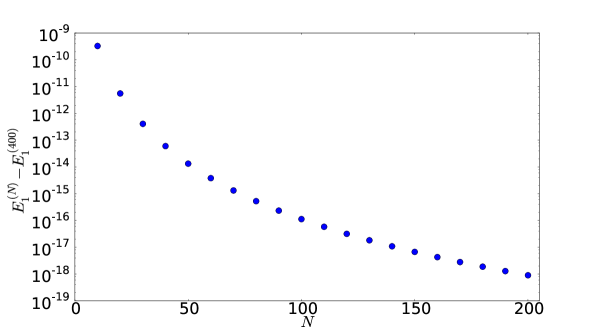
Figure 1: The difference $E_{1}^{(N)}-E_{1}^{(400)}$ for the lowest eigenvalue of the matrices representing $\hat{O}$ on a $N$ dimensional subspace.

This approach allows one to obtain very precise approximations also for the excited states of the string: in Fig. 2 we see that the 200 eigenvalues of the $200\times 200$ matrix representing $\hat{O}$ (circles) are very precise, even for the highest states. The few highest eigenvalues in the plot are obtained even more precisely using the diagonal matrix elements $\langle n|\hat{O}|n\rangle$ (dashed line), corresponding to using WKBPT to first order.

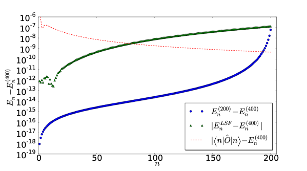
Figure 2: The difference $E_{n}-E_{n}^{(400)}$ for the lowest $200$ eigenvalues of the string of density (120). The circles correspond to $E_{n}$ calculated taking the eigenvalues of the $200\times 200$ matrix representing $\hat{O}$, whereas the triangles correspond to $E_{n}$ obtained using LSF with a grid of $2500$ points. The dashed curve corresponds to the difference $|\langle n|\hat{O}|n\rangle-E_{n}^{(400)}|$.

Actually one can use this spectral approach to obtain accurate results also for arbitrarily excited states: the crucial observation is that the matrix representing $\hat{O}$ becomes diagonally dominated for highly excited states. This can be understood in general terms remembering that the functions $\phi_{n}(x)$ of eq.(23) become eigenfunctions of $\hat{O}$ for $n\rightarrow\infty$.

Therefore, if we build a square $(2\bar{n}+1)\times(2\bar{n}+1)$ matrix, centered on the $n$ state, its eigenvalues and eigenvectors will provide increasingly better approximations to the exact eigenvalues and eigenfunctions of $\hat{O}$ as $n$ goes to infinity. In this way one may obtain precise estimates of the asymptotic behavior of the energies of this problem for $n\rightarrow\infty$.

For example, we may consider the three states corresponding to $n=10^{5}-1$, $10^{5}$ and $10^{5}+1$ and build a matrix centered at each of these states with $\bar{n}=100$.

To calculate the eigenvalues we have worked with the numerical matrices with a precision of $100$ digits and we have then extracted the coefficients of the asymptotic expansion with a fit, obtaining

$$E_{n} \approx 0.0018855885773910003409\ n^{2}-0.00026004036832396307366$$ (125)

$$+ \frac{0.00075459566769573983984}{n^{2}}+\dots\ .$$

These numerical coefficients should be compared with the exact coefficients calculated with WKBPT:

$$E_{n}=A_{1}n^{2}+A_{2}+\frac{A_{3}}{n^{2}}+\dots$$ (126)

where

$$A_{1} = \frac{9}{49\pi^{4}}\approx 0.0018855885773910003409$$ (127)

$$A_{2} = -\frac{1}{4\pi^{6}}\approx-0.00026004036832396307402\ ,$$ (128)

and

$$A_{3} = A_{3}^{(1)}+A_{3}^{(2)}\ .$$ (129)

The contribution to $A_{3}$ stemming from first order is easily calculated and reads:

$$A_{3}^{(1)} = -\frac{\sigma(L)}{4\pi^{2}}\left[V^{(1)}(\sigma(L))-V^{(1)}(0)\right]=\frac{3577}{512\pi^{8}}\approx 0.000736\ .$$ (130)

As we have seen before the contribution to $A_{3}$ stemming from second order involves a series

$$A_{3}^{(2)} = \frac{\sigma(L)^{2}}{\pi^{4}}\sum_{k=1}^{\infty}\frac{1}{2k^{2}}\left\{\left[\mathcal{F}\left(\frac{\sigma(L)}{\pi k},\sigma(L)\right)+\mathcal{F}\left(\frac{\sigma(L)}{\pi k},0\right)\right]^{2}\right.$$ (131)

$$- \left.\mathcal{F}\left(\frac{\sigma(L)}{2\pi k},\sigma(L)\right)\mathcal{F}\left(\frac{\sigma(L)}{2\pi k},0\right)\right\}\equiv\sum_{k=1}^{\infty}\gamma_{k}\ ,$$

and requires the calculation of $\mathcal{F}$.

For this example we find

$$\mathcal{G}(\upsilon,\sigma_{0}) = \frac{12\left(3\sigma_{0}+\pi^{3}\right)\upsilon}{\left(9\left(\sigma_{0}^{2}+\upsilon^{2}\right)+6\pi^{3}\sigma_{0}+\pi^{6}\right)^{2}}$$ (132)

and

$$\mathcal{F}(\upsilon,\sigma_{0}) = \frac{-2\Lambda{\rm Ci}(\Lambda)\sin(\Lambda)+2\Lambda{\rm Si}(\Lambda)\cos(\Lambda)-\pi\Lambda\cos(\Lambda)+2}{9\upsilon^{2}\Lambda}$$ (133)

where

$$\Lambda\equiv\frac{\pi^{3}+3\sigma_{0}}{3\upsilon}\ .$$ (134)

After substituting the expression for $\mathcal{F}$ inside the expression for $A_{3}^{(2)}$ we obtain an explicit expression for $\gamma_{k}$:

$$\gamma_{k} \equiv \frac{1}{14112\pi^{8}}\left[\left(8\pi k{\rm Ci}\left(\frac{k\pi}{7}\right)\sin\left(\frac{\pi k}{7}\right)+8\pi k{\rm Ci}\left(\frac{8k\pi}{7}\right)\sin\left(\frac{8\pi k}{7}\right)\right.\right.$$

$$- \left.\left.8\pi k{\rm Si}\left(\frac{k\pi}{7}\right)\cos\left(\frac{\pi k}{7}\right)-8\pi k{\rm Si}\left(\frac{8k\pi}{7}\right)\cos\left(\frac{8\pi k}{7}\right)\right.\right.$$

$$+ \left.\left.4\pi^{2}k\cos\left(\frac{\pi k}{7}\right)+4\pi^{2}k\cos\left(\frac{8\pi k}{7}\right)-63\right)^{2}\right.$$

$$- \left.32\left(2\pi k{\rm Ci}\left(\frac{2k\pi}{7}\right)\sin\left(\frac{2\pi k}{7}\right)-2\pi k{\rm Si}\left(\frac{2k\pi}{7}\right)\cos\left(\frac{2\pi k}{7}\right)\right.\right.$$

$$+ \left.\left.\pi^{2}k\cos\left(\frac{2\pi k}{7}\right)-7\right)\cdot\left(16\pi k{\rm Ci}\left(\frac{16k\pi}{7}\right)\sin\left(\frac{16\pi k}{7}\right)\right.\right.$$

$$- \left.\left.16\pi k{\rm Si}\left(\frac{16k\pi}{7}\right)\cos\left(\frac{16\pi k}{7}\right)+8\pi^{2}k\cos\left(\frac{16\pi k}{7}\right)-7\right)\right]\ .$$

We may estimate $A_{3}$ by restricting the series in $A_{3}^{(2)}$ to the first $N$ terms. For example, using $N=8000$ we obtain

$$A_{3}=A_{3}^{(1)}+A_{3}^{(2)}\approx\frac{3577}{512\pi^{8}}+\sum_{k=1}^{8000}\gamma_{k}\approx 0.00075459642403370616977\ .$$ (135)

A much better estimate may be obtained taking into account the asymptotic behavior of the $\gamma_{k}$ for $k\rightarrow\infty$:

$$\gamma_{k}\approx\frac{631561441}{294912\pi^{12}k^{4}}$$ (136)

and therefore we may write

$$A_{3}^{(2)}=\sum_{k=1}^{\infty}\gamma_{k}=\frac{631561441}{26542080\pi^{8}}+\sum_{k=1}^{\infty}\left[\gamma_{k}-\frac{631561441}{294912\pi^{12}k^{4}}\right]\ .$$ (137)

If we limit the sum to the first 8000 terms as before we obtain a more precise estimate for $A_{3}$:

$$A_{3} \approx A_{3}^{(1)}+\frac{631561441}{26542080\pi^{8}}+\sum_{k=1}^{8000}\left[\gamma_{k}-\frac{631561441}{294912\pi^{12}k^{4}}\right]$$ (138)

$$\approx 0.00075459642403521434583\ .$$

Therefore we see that the coefficients obtained with the fit are in very good agreement with the theoretical values obtained with WKBPT.

We will now use the very precise numerical results at our disposal to discuss the WKB-perturbation method and its improved version, which we have described in the previous sections.

We first concentrate on the bounds for the energy of the fundamental mode, starting with the one obtained using DPT, which largely overestimates the exact result

$$E_{1}\leq\frac{4}{15\pi}\ {\rm Si}(2\pi)-\frac{4}{15\pi}\ {\rm Si}(4\pi)+\frac{7}{30\pi^{4}}+\frac{1}{15\pi^{2}}\approx 0.002868007277\ .$$ (139)

We should not be surprised by this result since the density of the string varies strongly on the domain and therefore density perturbation theory is not applicable.

We now discuss the first bound obtained WKBPT. First we make an important observation: since $V(\sigma)$ is negative on the whole string, then $E_{n}^{(1)}$ in eq. (59) is also negative. Moreover, for the modes of the string which are arbitrarily excited the ratio $E_{n}^{(1)}/E_{n}^{(0)}$ becomes arbitrarily small, while $E_{n}^{(0)}$ becomes arbitrarily accurate as $n\rightarrow\infty$, thus we may conclude that the $E_{n}^{(0)}$ are upper bounds to the energies of the string as $n\rightarrow\infty$. We have numerically tested this conjecture using the eigenvalues of the $400\times 400$ matrix representing $\hat{O}$ and we have found that it actually holds even for the intermediate states.

The WKBPT bound is readily obtained using the matrix element previously calculated:

$$E_{1} \leq \frac{9\pi}{49\pi^{5}}+\frac{4}{49\pi^{5}}\left[\left({\rm Ci}\left(\frac{16\pi}{7}\right)-{\rm Ci}\left(\frac{2\pi}{7}\right)\right)\cos\left(\frac{3\pi}{14}\right)\right.$$ (140)

$$+ \left.\left({\rm Si}\left(\frac{2\pi}{7}\right)-{\rm Si}\left(\frac{16\pi}{7}\right)\right)\sin\left(\frac{3\pi}{14}\right)\right]\approx 0.001745807766\ ,$$

which is much tighter than the bound obtained with DPT. It is also interesting to compare this result with the WKB result to first order:

$$E_{1}^{{\rm WKB}(0)}+E_{1}^{{\rm WKB}(1)}=\frac{9}{49\pi^{4}}-\frac{1}{4\pi^{6}}\approx 0.00162555\ ,$$ (141)

which is less precise than the previous one and falls below the exact value.

As we have discussed before, one may still obtain better bounds using the first order WKBPT wave function as trial solution: in the present example, the matrix elements $\langle k|V|l\rangle$ are known explicitly and therefore the bound can be calculated easily. Notice that the variational bound holds also when a finite number of terms is used in the series appearing in $\langle\hat{O}\rangle_{\Psi}$.

In Table 2 we report the variational bounds obtained restricting the sum up to $k=N$ terms and compare the results with the ”exact” numerical value quoted by Bender and Orszag and with the even more precise values that have been obtained using a collocation approach based on the LSF functions of ref. [16] with grids with $2000$ and $2500$ points (the use of collocation in the numerical solution of the problem of an inhomogeneous string is illustrated in ref. [1]). Notice that for $N>20$ the variational bound does not improve, signaling the need for a more refined ansatz.

Table 2: Variational bounds using first order WKBPT to the energy of the fundamental mode of a string with density $\rho(x)=\left(x+\frac{3}{2}\pi\right)^{4}$. The notation $[-n]$ means $10^{-n}$.

$N$	$E_{1}(N)$	$E_{1}(N)-E_{1}^{\rm LSF_{2500}}$
2	0.0017442945174961415	2.81 [-7]
3	0.0017440904942458490	7.70 [-8]
4	0.0017440396134339554	2.61 [-8]
5	0.0017440245258144354	1.10 [-8]
6	0.0017440189344824756	5.39 [-9]
7	0.0017440167007034352	3.16 [-9]
8	0.0017440156851693774	2.14 [-9]
9	0.0017440152042467934	1.66 [-9]
10	0.0017440149552016950	1.41 [-9]
20	0.0017440146360548171	1.09 [-9]
30	0.0017440146309786759	1.09 [-9]
40	0.0017440146306353234	1.09 [-9]
50	0.0017440146305891107	1.09 [-9]
ref. [3]	0.00174401
LSF2000	0.0017440135432079554
LSF2500	0.0017440135430055502

In Table 3 we report the energies of selected modes of the string considered by Bender and Orszag, calculated with WKBPT to first order and second orders (second and fourth columns), with the asymtotic formulas $A_{1}n^{2}+A_{2}$ and $A_{1}n^{2}+A_{2}+\frac{A_{3}}{n^{2}}$ (third and fifth columns) and with the LSF collocation method with a grid with $2500$ points (sixth column). Clearly the second order WKBPT results are very precise even for the lowest modes: this fact signals that the dominant contributions to the asymptotic coefficients $A_{j}$, with $j=4,5,\dots$, may be (at least in principle) calculated using the expression of the energy to second order in WKBPT, in analogy with what we have done in the calculation of $A_{3}$.

Table 3: Comparison of the energies for selected modes of a string with density $\rho(x)=\left(x+\frac{3}{2}\pi\right)^{4}$ calculated with WKBPT to first and second orders (second and fourth columns), with the asymtotic formulas $A_{1}n^{2}+A_{2}$ and $A_{1}n^{2}+A_{2}+\frac{A_{3}}{n^{2}}$ (third and fifth columns) and with the LSF collocation method with a grid with $2500$ points (sixth column). The series in the second order WKBPT term is restricted to the 20 closest states.

$n$	$E_{n}^{({\rm I})}$	$A_{1}n^{2}+A_{2}$	$E_{n}^{({\rm II})}$	$A_{1}n^{2}+A_{2}+\frac{A_{3}}{n^{2}}$	$E_{n}^{\rm LSF_{2500}}$
1	0.00174581	0.00162555	0.00174405	0.00238014	0.00174401
2	0.00734927	0.00728231	0.00734864	0.00747096	0.00734866
3	0.01675247	0.01671026	0.01675237	0.01679410	0.01675238
4	0.02993818	0.02990938	0.02993827	0.02995654	0.02993828
5	0.04690044	0.04687967	0.04690060	0.04690986	0.04690060
6	0.06763676	0.06762115	0.06763693	0.06764211	0.06763693
7	0.09214593	0.09213380	0.09214609	0.09214920	0.09214609
8	0.12042730	0.12041763	0.12042744	0.12042942	0.12042744
9	0.15248051	0.15247263	0.15248064	0.15248195	0.15248064
10	0.18830534	0.18829882	0.18830546	0.18830636	0.18830546
20	0.75397717	0.75397539	0.75397721	0.75397728	0.75397721
30	1.69677048	1.69676968	1.69677050	1.69677052	1.69677050
40	3.01668214	3.01668168	3.01668215	3.01668216	3.01668215
50	4.71371167	4.71371140	4.71371170	4.71371170	4.71371170

We will now discuss the bound obtained using the improved WKBPT approach (iWKBPT), eq. (71). We consider the trial density

$$\tilde{\rho}(x)=\rho(x)\ \left[\sum_{j=0}^{N}a_{j}x^{j}\right]^{2}\ ,$$ (142)

where the $a_{j}$ are $N+1$ real parameters to be determined variationally.

Clearly choosing $a_{0}=1$ and $a_{j}=0$ for $j>0$ (corresponding to $N=0$), $\tilde{\rho}(x)$ reduces to the physical density: in this case we recover the simpler bound of WKBPT.

In Table 4 we report the energy corresponding to a set of values of the ”optimal” $a_{i}$ and the numerical value of the quantity $\frac{\sigma(L)^{2}}{\tilde{\sigma}(L)^{3}}\int_{-L}^{+L}\frac{\tilde{\rho}(x)^{3/2}}{\rho(x)}dx$, which determines the asymptotic behavior of the energies.

For $N=10$ the first 17 digits of the variational energy agree with those of the energy of eq. (124); the case $N=0$ corresponds to normal WKBPT, which uses the physical density as $\tilde{\rho}(x)$.

Table 4: The variational estimate for the energy of the fundamental mode of the string of density $\rho(x)=\left(x+\frac{3}{2}\pi\right)^{4}$ and the quantity $\frac{\sigma(L)^{2}}{\tilde{\sigma}(L)^{3}}\int_{-L}^{+L}\frac{\tilde{\rho}(x)^{3/2}}{\rho(x)}dx$ determining the asymptotic behavior of the spectrum.

$N$	$E_{1}^{\rm iWKBPT}$	$E_{1}^{\rm iWKBPT}-E_{1}^{(200)}$	$\frac{\sigma(L)^{2}}{\tilde{\sigma}(L)^{3}}\int_{-L}^{+L}\frac{\tilde{\rho}(x)^{3/2}}{\rho(x)}dx$
0	0.00174580776578874	1.79 [-6]	1.00000
1	0.00174408029127495	6.67 [-8]	1.00076
2	0.00174402710509883	1.36 [-8]	1.00088
3	0.00174401553013316	1.99 [-9]	1.00088
4	0.00174401377197412	2.28 [-10]	1.00088
5	0.00174401354435309	5.35 [-13]	1.00088
6	0.00174401354405299	2.34 [-13]	1.00088
7	0.00174401354384465	2.61 [-14]	1.00088
8	0.00174401354382102	2.47 [-15]	1.00088
9	0.00174401354381886	3.12 [-16]	1.00088
10	0.00174401354381859	3.70 [-17]	1.00088
$E_{1}^{(200)}$	0.00174401354381855

In Fig. 3 we plot the physical density $\rho(x)=\left(x+\frac{3}{2}\pi\right)^{4}$ (solid line) and compare it with the optimal trial density obtained with the iWKBPT bound using $N=10$ parameters (dashed line). This density approximates the effective density for the fundamental mode of $\hat{O}$.

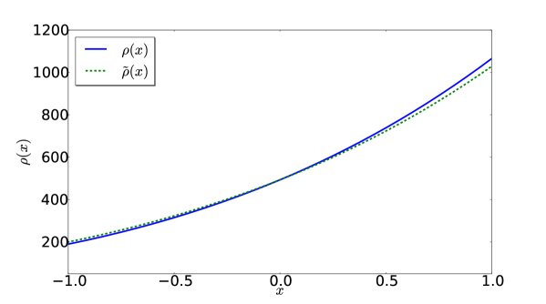
Figure 3: Comparison between the physical density $\rho(x)=\left(x+\frac{3}{2}\pi\right)^{4}$ (solid line) and the optimal trial density obtained with the iWKBPT bound with $N=10$ (dashed line).

Using the transformation discussed by in ref. [8] we may obtain refined bounds for the energy of the fundamental mode of our string, studying an isospectral string of density

$$\bar{\rho}(x)=\frac{16(\pi\alpha+1)^{2}(\pi(2\alpha(2x+\pi)+3)+2x)^{4}}{(\alpha(2x+\pi)+2)^{8}}\ .$$ (143)

In Table 5 we report the values of these bounds obtained by minimizing the expectation value of $\bar{\hat{O}}$ in the fundamental mode of $\tilde{Q}$ where the density $\tilde{\rho}(x)$ has the same form considered before. The minimization is done with respect to $\alpha$ and to the parameters in $\tilde{\rho}(x)$. In the fifth column we report the optimal value of $\alpha$, for a set of $N$ parameters $a_{i}$. The minimization of the expectation value for a set of $N+1$ parameters (the $N$ parameters $a_{i}$ and $\alpha$) is done using the $N$ parameters of the previous solution as a starting point.

Notice that the result obtained for $N=0$ is roughly an order of magnitude more precise than the corresponding result in Table 4 and that it retains the exact asymptotic behavior.

On the other hand the results obtained for $N\geq 7$ have a larger error than the corresponding results obtained in Table 4: this means that the solution that we have found corresponds to a local minimum of the expectation value. On the other hand, we should observe that the asymptotic behavior of the spectrum obtained in table 5 for $N\geq 7$ more accurate than the corresponding behavior in Table 4.

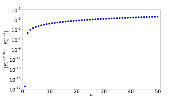
Figure 4: $|E_{n}^{iWKBPT}-E_{n}^{exact}|$ for the case of a string with density $\rho(x)=\left(x+\frac{3}{2}\pi\right)^{4}$. The iWKBPT results are obtained using an optimal density with $N=10$ parameters.

Table 5: The variational estimate for the energy of the fundamental mode of the string of density $\bar{\rho}(x)=\frac{16(\pi\alpha+1)^{2}(\pi(2\alpha(2x+\pi)+3)+2x)^{4}}{(\alpha(2x+\pi)+2)^{8}}$ and the quantity $\frac{\sigma(L)^{2}}{\tilde{\sigma}(L)^{3}}\int_{-L}^{+L}\frac{\tilde{\rho}(x)^{3/2}}{\rho(x)}dx$ determining the asymptotic behaviour of the spectrum.

$N$	$E_{1}^{\rm iWKBPT}$	$E_{1}^{\rm iWKBPT}-E_{1}^{(200)}$	$\frac{\sigma(L)^{2}}{\tilde{\sigma}(L)^{3}}\int_{-L}^{+L}\frac{\tilde{\rho}(x)^{3/2}}{\rho(x)}dx$	$\alpha$
0	0.00174418771063455	1.74 [-7]	1.00000	-0.00840
1	0.00174404317510904	2.96 [-8]	1.00415	0.01082
2	0.00174401638359089	2.84 [-9]	1.00532	-0.02892
3	0.00174401358072024	3.69 [-11]	1.00930	-0.03528
4	0.00174401356813542	2.43 [-11]	1.02434	-0.05076
5	0.00174401354405135	2.33 [-13]	1.00016	-0.00565
6	0.00174401354405132	2.33 [-13]	1.00016	-0.00565
7	0.00174401354385037	3.18 [-14]	1.00016	-0.00566
8	0.00174401354382192	3.37 [-15]	1.00016	-0.00566
9	0.00174401354381896	4.10 [-16]	1.00016	-0.00566
10	0.00174401354381860	5.05 [-17]	1.00016	-0.00566
$E_{1}^{(200)}$	0.00174401354381855

6.5 A string with rapidly oscillating density

We will now study a string of unit length ($|x|\leq 1/2$) and with a rapidly oscillating density

$$\rho(x)=\left(2+\sin(100\pi x)\right)^{2}\ .$$ (144)

In this case one has

$$\sigma(x)=1+2x+\frac{\sin^{2}(50\pi x)}{50\pi}\ .$$ (145)

It is known that the solutions for strings with rapidly oscillating density have peculiar properties: in particular the solutions whose wavelength corresponds roughly to the typical size of the density oscillations are localized at the ends of the strings [2, 17, 18].

Before we apply the results of the previous sections to the study of this string we wish to obtain numerical results which will be useful to assess the precision of the analytical methods: as for the previous example we have used a collocation approach based on LSF with an homogeneous grid of $2500$ points. The grid spacing $h=2L/N$ is sufficiently fine to obtain precise results for the first few hundreds of states; in particular, the energy of the fundamental mode obtained with this grid is

$$E_{1}^{LSF_{2500}}=2.1931584082\ .$$ (146)

The quality of the variational bounds obtained with the different approaches will be established using this value.

In Fig. 5 we display the numerical values of the square roots of the first $350$ energies of this string obtained with the LSF collocation using $2500$ points (plus symbols) and we compare them with the exact leading asymptotic behavior $k_{n}=n\pi/2$ (dashed line). Gaps are observed in correspondence to quantum numbers which are multiples of $50$: as we have anticipated these gaps occurr because of the appearance of localized solutions at one of the ends of the string.

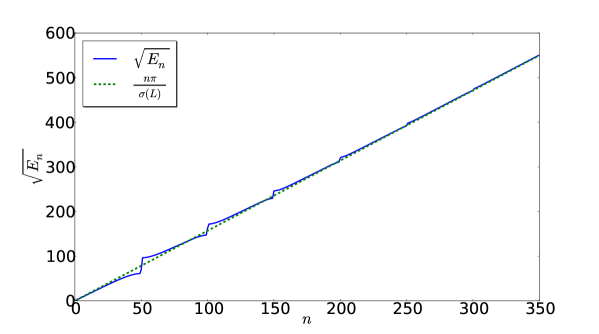
Figure 5: Wave numbers of the string with density $\rho(x)=\left(2+\sin(100\pi x)\right)^{2}$ obtained with LSF with a grid of $2500$ points. The dashed line is the asymptotic behavior $k_{n}=n\pi/\sigma(L)$.

In Fig. 6 we display three solutions of the Helmholtz equation for the string with density $\rho(x)=\left(2+\sin(100\pi x)\right)^{2}$, obtained using LSF collocation with a grid of $2500$ points. The mode for $n=50$ is localized on the left end of the string, while the modes corresponding to $n=49$ and $n=51$ extend over all the string. It is instructive to decompose these solutions in terms of the modes of an uniform string: we may expect that the modes of this string which are not localized may be described in terms of few modes of an uniform string, whereas the modes of this string which are localized necessarily involve a great number of modes of the uniform string.

This analysis can be carried out rapidly and efficiently using the results of the LSF collocation, and at no extra computational cost. The fundamental observation is that the LSF are defined as

$$s_{k}(x)\equiv\frac{2L}{N}\sum_{n=1}^{N}\psi_{n}(x_{k})\psi_{n}(x)\ ,$$ (147)

where $\psi_{n}(x)\equiv\sqrt{\frac{1}{L}}\sin\frac{n\pi(x+L)}{2L}$ are the eigensolutions of the uniform string on $-L\leq x\leq L$ with Dirichlet boundary conditions at $x=\pm L$. The $x_{k}\equiv 2Lk/N$ are the uniformly distributed grid points.

A function $f(x)$ whose values are known at the grid points may then be approximated at arbitrary points in the domain through the interpolation formula

$$f(x) \approx \sum_{k=-N/2+1}^{N/2-1}f(x_{k})s_{k}(x)$$ (148)

$$= \sum_{n=1}^{N}\left[\frac{2L}{N}\sum_{k=-N/2+1}^{N/2-1}f(x_{k})\psi_{n}(x_{k})\right]\psi_{n}(x)\ ,$$

where the terms inside the parenthesis are the approximate Fourier coefficients of $f(x)$. In the case that we are considering $f(x_{k})$ is just the $k^{th}$ entry of one of the eigenvectors of the $(N-1)\times(N-1)$ matrix that we have obtained from the discretization of the Helmholtz equation, multiplied by a factor $\sqrt{N/2L}$, and $\psi_{n}(x_{k})$ is the $k^{th}$ entry of the vector obtained evaluating the $n^{th}$ eigensolution of the uniform string on the $k^{th}$ grid point. The calculation of the Fourier coefficients thus involves (apart from a multiplicative factor) the multiplication of two vectors, which have been already calculated.

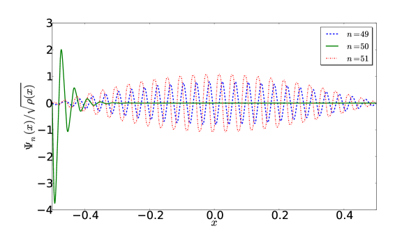
Figure 6: Solutions for the modes $49$,$50$ and $51$ of the string with density $\rho(x)=\left(2+\sin(100\pi x)\right)^{2}$ obtained with LSF with a grid of $2500$ points.

In Fig. 7 and 8 we display the approximate Fourier coefficients for the solutions of Fig.6 for $n$ odd and even respectively, obtained with LSF on a grid of $2500$ points. The coefficients of the solutions corresponding to $n=49$ and $n=51$ behave very differently for odd and even modes while the coefficients of the localized solution, corresponding to $n=50$, behave similarly in the two cases and decay slowly.

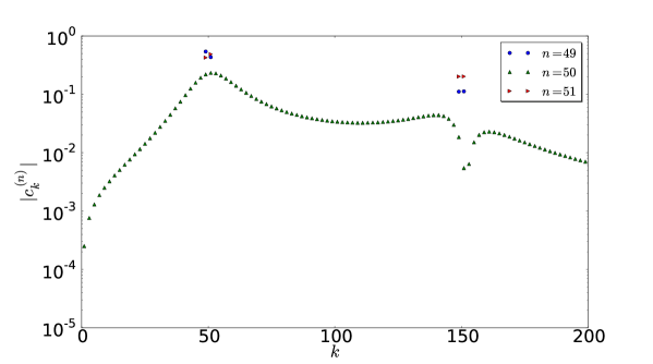
Figure 7: Approximate odd Fourier coefficients for the modes $49$,$50$ and $51$ of the string with density $\rho(x)=\left(2+\sin(100\pi x)\right)^{2}$ obtained with LSF with a grid of $2500$ points.

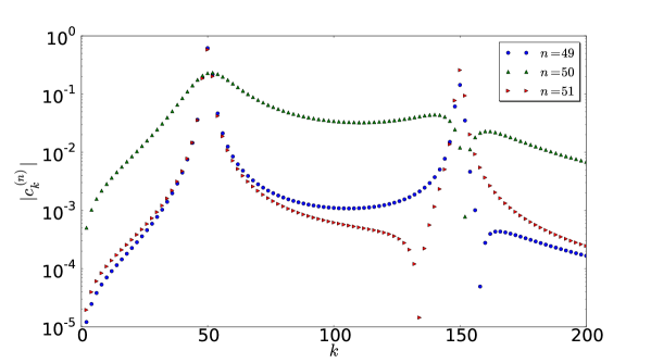
Figure 8: Approximate even Fourier coefficients for the modes $49$,$50$ and $51$ of the string with density $\rho(x)=\left(2+\sin(100\pi x)\right)^{2}$ obtained with LSF with a grid of $2500$ points.

We may now discuss the bounds for the energy of the fundamental mode obtained using the different approaches outlined in the previous sections; in the case of DPT one uses the fundamental solution of a uniform string as variational ansatz and obtains a bound which falls quite above the exact energy:

$$E_{1}\leq 6335.15\ .$$ (149)

The situation is only partially better using WKBPT: the ”potential” $V(x)$ corresponding to this density is

$$V(x)=-\frac{1250\pi^{2}(8\sin(100\pi x)+\cos(200\pi x)+5)}{(\sin(100\pi x)+2)^{4}}$$ (150)

and using the formula derived earlier the bound reads

$$E_{1}\leq 1189.60\ .$$ (151)

This large bound originates almost entirely from the first order contribution

$$E_{1}^{(1)}=\frac{2}{\sigma(L)}\int_{-L}^{L}\sqrt{\rho(x)}V(x)\sin^{2}\frac{\pi\sigma(x)}{\sigma(L)}dx\approx\frac{1}{\sigma(L)}\int_{-L}^{L}\sqrt{\rho(x)}V(x)dx\ .$$ (152)

This result clearly suggests that the WKBPT describes poorly the lowest part of the spectrum of this system, although the basis of the eigenfunctions of $\hat{Q}$ reproduces the asymptotic behavior of the high part of the spectrum of $\hat{O}$. Both bounds calculated so far are clearly useless!

In the iWKBPT approach one may use an effective density $\tilde{\rho}(x)$, different from the physical density and specific to a given state, to improve the description of the lowest energy solutions. As we have seen in the case of WKBPT discussed above, the large values obtained in the bound originate from the rapid oscillations of the density: one should therefore pick an effective density $\tilde{\rho}(x)$ for which these contributions are suppressed.

An useful ansatz is

$$\tilde{\rho}(x)\approx\rho(x)^{2}\ ,$$ (153)

since it cancels large contributions to the expectation value of $\hat{O}$ stemming from the oscillations of the density.

The bound for the fundamental energy obtained in this case is much closer to the numerical result obtained with collocation

$$E_{1}\leq 3.07325\ ,$$ (154)

although the quality of this bound is not competing with the precision of the numerical result.

We will now show that it is possible to obtain extremely precise variational bounds, choosing a suitable variational ansatz, given by the trial function (normalized to one) as

$$\psi_{1}^{(trial)}(x)=\frac{\sqrt{2}}{3}\sqrt{\rho(x)/L}\sin\left[\pi\frac{x+L}{2L}\right]\ .$$ (155)

A simple calculation shows that the bound is this case is

$$E_{1}\leq\frac{2}{9}\pi^{2}\approx 2.19325\ ,$$ (156)

where the first four digits of the rhs are correct.

Can we still improve this bound? Yes, we can: we can use Theorem 1 of ref. [1] to obtain further analytical improvements of this bound. Using the notation of that paper we set $\xi_{0}(x)\equiv\psi_{1}^{(trial)}(x)$ and obtain refined approximations for the fundamental solution applying the iterative equation eq. (92).

The bounds obtained in this way are given in Table 6: after $7$ iterations it appears that the first $19$ digits have converged. In principle the iterations can be performed to arbitrary orders, as long as one is able to perform the integrals analytically . A comparison with the LSF result shows that the first 10 digits of the value obtained with collocation are correct.

Table 6: Variational bounds for the energy of the fundamental mode of the string of unit length of density $\rho(x)=\left(2+\sin(100\pi x)\right)^{2}$ obtained using Theorem 1 of ref. [1] with the initial trial function in eq. (155).

$n$	$E_{1}$
0	2.1932454224643019153
1	2.1931584087453807530
2	2.1931584087440065685
3	2.1931584087439513989
4	2.1931584087439479612
5	2.1931584087439477463
6	2.1931584087439477329
7	2.1931584087439477320

Having obtained accurate numerical solutions for the low lying states of this string, we may look for the effective densities corresponding to these states. In this case one needs to solve numerically the equation

$$\frac{\tilde{\sigma}(x)}{\tilde{\sigma}(L)} = \frac{1}{2\pi}\sin\frac{2\pi\tilde{\sigma}(x)}{\tilde{\sigma}(L)}+\int_{-L}^{x}\left[\psi_{1}^{(trial)}(y)\right]^{2}dy\ .$$ (157)

The effective density is then obtained through the relation $\tilde{\sigma}^{\prime}(x)=\sqrt{\tilde{\rho}(x)}$. In Fig.9 we show the effective densities for the first four solutions, scaled by the factor $\rho(x)^{2}$, which we have already seen to be a good approximation: as a matter of fact we may notice that $\tilde{\rho}_{1}(x)/\rho^{2}(x)$ is almost flat, with oscillations only at the ends of the string.

In the case of the remaining states we notice a very peculiar behavior of the effective density, which develops $n-1$ zeroes in the domain, which also coincide with the zeroes of the solution (the zeroes of the eigenfunctions of $\tilde{\hat{Q}}$ correspond either to the zeroes of the trigonometric function or to the zeroes of the effective density, as in the present case).

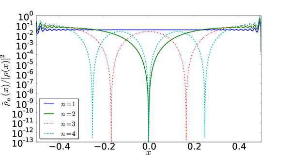
Figure 9: Effective densities for the first four solutions of the string with density $\rho(x)=\left(2+\sin(100\pi x)\right)^{2}$ obtained with LSF with a grid of $2500$ points.

In Fig. 10 we display the same ratio for the modes corresponding to $n=49$, $50$ and $51$. The effective density of the mode $50$ is clearly localized at the left end of the string.

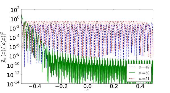
Figure 10: Effective densities for the solutions $49$, $50$ and $51$ of the string with density $\rho(x)=\left(2+\sin(100\pi x)\right)^{2}$ obtained with LSF with a grid of $2500$ points.

7 Low and high energy asymptotics for strings with rapidly oscillating density

In this section we use the theorems of Section 5 to obtain the low energy asymptotics of a string with density 

$$\rho(x) = 2+\sin\left(\frac{2\pi\left(x+\frac{1}{2}\right)}{\epsilon}\right)$$ (158)

with $\epsilon\rightarrow 0^{+}$ and $x^{2}\leq 1/4$.

As we have seen through Theorem 1 it is possible to obtain a sequence of functions which converge to the fundamental solution of $\hat{O}$ provided that the initial trial function is not orthogonal to it. Therefore we may consider the function

$$\xi_{0}(x)=\sqrt{\rho(x)}\sin\frac{\pi(x+1/2)}{2L}\ .$$ (159)

Actually this $\xi_{0}(x)$ not only is not orthogonal to the exact fundamental mode of $\hat{O}$, but it also tends to become an exact eigenfunction of $\hat{O}$ in the limit $\epsilon\rightarrow 0^{+}$.

We can see this by calculating

$$\frac{\hat{O}\xi_{0}(x)}{\xi_{0}(x)}=\frac{\pi^{2}}{2+\sin\left(\frac{2\pi\left(x+\frac{1}{2}\right)}{\epsilon}\right)}\approx\frac{\pi^{2}}{2}\ ,$$ (160)

having substituted in the last expression the highly oscillatory term $\sin\left(\frac{2\pi\left(x+\frac{1}{2}\right)}{\epsilon}\right)$ with its average value on the interval.

We thus use Theorem 1 to build increasingly refined approximations of the fundamental solution of $\hat{O}$ corresponding to the density (158) in the limit $\epsilon\rightarrow 0^{+}$. For instance, after one iteration we obtain the function:

$$\xi_{1}(x) = \frac{\sqrt{\sin\left(\frac{2\pi\left(x+\frac{1}{2}\right)}{\epsilon}\right)+2}}{2\pi^{2}\left(\epsilon^{2}-4\right)^{2}}\ \left[4\epsilon^{3}(2x+1)\cos\left(\frac{2\pi}{\epsilon}\right)\right.$$ (161)

$$+ \left.\epsilon^{2}\left(4\epsilon(2x-1)+(\epsilon-2)^{2}\sin\left(\frac{\pi((\epsilon+2)x+1)}{\epsilon}\right)\right.\right.$$

$$+ \left.\left.(\epsilon+2)^{2}\sin\left(\frac{\pi(-\epsilon x+2x+1)}{\epsilon}\right)\right)+4\left(\epsilon^{2}-4\right)^{2}\cos(\pi x)\right]\ .$$

We have also calculated explicitly the functions corresponding to two and three iterations, although their expressions are much lengthier and therefore we will not report them here.

We will instead calculate the expectation value of $\hat{O}$ in these functions, thus obtaining an asymptotic expression for the fundamental energy of this string in the limit $\epsilon\rightarrow 0^{+}$.

We report here these expressions:

$$\langle\hat{O}\rangle_{\xi_{0}} \equiv \frac{\int_{-L}^{+L}\xi_{0}(x)\hat{O}\xi_{0}(x)dx}{\int_{-L}^{+L}\xi_{0}(x)^{2}dx}\approx\frac{\pi^{2}}{2}+\frac{1}{4}\pi\sin^{2}\left(\frac{\pi}{\epsilon}\right)\epsilon^{3}+\frac{1}{4}\pi\sin^{2}\left(\frac{\pi}{\epsilon}\right)\epsilon^{5}+\dots$$ (162)

$$\langle\hat{O}\rangle_{\xi_{1}} \equiv \frac{\int_{-L}^{+L}\xi_{1}(x)\hat{O}\xi_{1}(x)dx}{\int_{-L}^{+L}\xi_{1}(x)^{2}dx}\approx\frac{\pi^{2}}{2}-\frac{\pi^{2}}{64}\epsilon^{2}+\frac{1}{4}\pi\sin^{2}\left(\frac{\pi}{\epsilon}\right)\epsilon^{3}-\frac{15\pi^{2}}{1024}\epsilon^{4}$$ (163)

$$+ \frac{\pi\left(5\sin\left(\frac{4\pi}{\epsilon}\right)-116\cos\left(\frac{2\pi}{\epsilon}\right)+116\right)}{1024}\epsilon^{5}+\dots$$

$$\langle\hat{O}\rangle_{\xi_{2}} \equiv \frac{\int_{-L}^{+L}\xi_{2}(x)\hat{O}\xi_{2}(x)dx}{\int_{-L}^{+L}\xi_{2}(x)^{2}dx}\approx\frac{\pi^{2}}{2}-\frac{\pi^{2}}{64}\epsilon^{2}+\frac{1}{4}\pi\sin^{2}\left(\frac{\pi}{\epsilon}\right)\epsilon^{3}-\frac{15\pi^{2}}{1024}\epsilon^{4}$$ (164)

$$+ \frac{\pi\left(5\sin\left(\frac{4\pi}{\epsilon}\right)-116\cos\left(\frac{2\pi}{\epsilon}\right)+116\right)}{1024}\epsilon^{5}+\dots$$

As we can see the expectation value of $\hat{O}$ has converged to order $\epsilon^{5}$ after just one iteration; thus we can conclude that, for $\epsilon\rightarrow 0^{+}$, the energy of the fundamental mode goes like

$$E_{1} \approx \frac{\pi^{2}}{2}-\frac{\pi^{2}}{64}\epsilon^{2}+\frac{1}{4}\pi\sin^{2}\left(\frac{\pi}{\epsilon}\right)\epsilon^{3}-\frac{15\pi^{2}}{1024}\epsilon^{4}$$ (166)

$$+ \frac{\pi\left(5\sin\left(\frac{4\pi}{\epsilon}\right)-116\cos\left(\frac{2\pi}{\epsilon}\right)+116\right)}{1024}\epsilon^{5}+O\left[\epsilon^{6}\right]\ .$$

This result may be compared with eq.(3.33) of Ref.[2], which reports $\sqrt{E_{1}}$ to order $O\left[\epsilon^{4}\right]$ for this example.

Let us now derive the asymptotics for the low energy states of this string; in this case we use Theorem 3 and consider the trial function

$$\eta_{0}(x)=\sqrt{2+\sin\left(\frac{2\pi\left(x+\frac{1}{2}\right)}{\epsilon}\right)}\ \sin\left(\frac{\pi\left(x+\frac{1}{2}\right)}{{\bar{L}}+\frac{1}{2}}\right)\ ,$$ (167)

with $\eta_{0}(-L)=\eta_{0}(\bar{L})=0$. Notice that $\eta_{0}(L)=0$ only for $\bar{L}=-\frac{1}{2}+\frac{1}{n}$, with $n=1,2,\dots$ and

$$\frac{\hat{O}\eta_{0}(x)}{\eta_{0}(x)}=\frac{n^{2}\pi^{2}}{2+\sin\left(\frac{2\pi x+\pi}{\epsilon}\right)}\approx\frac{n^{2}\pi^{2}}{2}\ ,$$ (168)

meaning that for $\epsilon\rightarrow 0^{+}$, the $\eta_{0}(x)$ for $\bar{L}=-\frac{1}{2}+\frac{1}{n}$ converges to the $n^{th}$ solution for this string (again we are substituting the oscillating factor with its average value on the interval in this limit).

We may now apply Theorem 3: after one iteration we obtain the function

$$\eta_{1}(x) = \frac{(2{\bar{L}}+1)^{2}\sqrt{\sin\left(\frac{2\pi\left(x+\frac{1}{2}\right)}{\epsilon}\right)+2}}{8\pi^{2}(\epsilon-2{\bar{L}}-1)^{2}(\epsilon+2{\bar{L}}+1)^{2}}\left[4\epsilon^{3}(2x+1)\cos\left(\frac{2\pi{\bar{L}}+\pi}{\epsilon}\right)\right.$$ (169)

$$+ \left.\epsilon^{2}(\epsilon+2{\bar{L}}+1)^{2}\cos\left(\frac{\pi(2x+1)(\epsilon-2{\bar{L}}-1)}{2\epsilon{\bar{L}}+\epsilon}\right)\right.$$

$$+ \left.\epsilon^{2}(\epsilon-2{\bar{L}}-1)^{2}\cos\left(\frac{\pi({\bar{L}}(-2\epsilon+4x+2)+2(\epsilon+1)x+1)}{2\epsilon{\bar{L}}+\epsilon}\right)\right.$$

$$+ \left.4\left(2\epsilon^{3}(x-{\bar{L}})+\left(\epsilon^{2}-(2{\bar{L}}+1)^{2}\right)^{2}\sin\left(\frac{2\pi x+\pi}{2{\bar{L}}+1}\right)\right)\right]\ .$$

The zeroes of the equation

$$\eta_{1}(L)=0$$ (170)

will now provide improved values for $\bar{L}$ and for the energies.

In Fig.11 we display $\eta_{1}(L)$ corresponding to $\epsilon=1/50$, as a function of $(L+\bar{L})$: the spikes of the curve correspond to zeroes of $\eta_{1}(L)$, located at specific values of $\bar{L}$. Corresponding to each value Theorem 3 provides an approximate eigenvalue and eigensolution to the string problem.

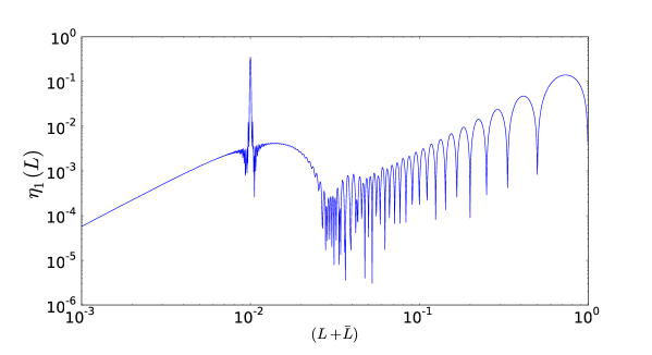
Figure 11: The function of eq.(169) evaluated at $x=L$, for $\epsilon=1/50$ as a function of $(L+\bar{L})$.

In Table 7 we report the values of $\bar{L}$ corresponding to the first 20 zeroes of $\eta_{1}(L)$ and the corresponding energies obtained by calculating the expectation value of $\hat{O}$ in the corresponding state; the last column contains the precise numerical results obtained with LSF collocation with a grid of $2500$ points. Thus we see that Theorem 3 provides rather precise results for a large number of states just after one iteration.

Table 7: Approximate energies of a string with density (158) with $\epsilon=1/50$ obtained with Theorem 3 (third column) and corresponding values obtained with LSF on a grid of $2500$ points (fourth column). The second column contains the values of $\bar{L}$ for which $\eta_{1}(L)=0$ (see the figure).

$n$	$\bar{L}$	$E_{n}$	$E_{n}^{{\rm LSF_{2500}}}$
1	0.50000000000000	4.93474049237786	4.93474049164385
2	0.00000254847810	19.7382203568987	19.7382203589595
3	-0.16666618871377	44.4082063869071	44.4082063970937
4	-0.25000000000000	78.9409479076410	78.9409485235574
5	-0.30001279890522	123.331046653456	123.331137037346
6	-0.33332758093170	177.571827239743	177.571841516164
7	-0.35716402051048	241.652567358357	241.654430048229
8	-0.37497950785717	315.566145317546	315.568467036379
9	-0.38888465796479	399.301373439805	399.301587271749
10	-0.39993517619554	492.724112367784	492.839343430514
11	-0.40908535234753	596.163807132223	596.165023435926
12	-0.41659695736991	708.868637232727	709.259433238896
13	-0.42315478442053	831.113631633346	832.100639666984
14	-0.42856494498590	964.660849364111	964.663666640351
15	-0.43336143492296	1106.57429450867	1106.92013667688
16	-0.43735701119023	1249.09849824817	1258.83784766743
17	-0.44135393715531	1396.14689996551	1420.38027258297
18	-0.44431129182849	1574.93187010870	1591.50596694241
19	-0.44739462363259	1770.83890618558	1772.16786511172
20	-0.45000000000000	1962.04796373469	1962.31244196980

We look for approximate solutions of the form

$$\bar{L}=\left(-\frac{1}{2}+\frac{1}{n}\right)+\delta\bar{L}$$ (171)

where $\delta\bar{L}$ is a correction. To leading order we have

$$\delta\bar{L}\approx\frac{\epsilon^{3}(-1)^{-n}n\left(n\cos\left(\frac{2\pi}{\epsilon n}\right)+(-1)^{n}\cos\left(\frac{2\pi}{\epsilon}\right)+n-1\right)}{8\pi}\ .$$ (172)

Notice that $\delta\bar{L}=0$ for $n=1$, as it should be.

Working to order $\epsilon^{3}$ we have calculated the expectation value of $\hat{O}$ in $\eta_{1}(x)$ to order $\epsilon^{3}$:

$$\langle\hat{O}\rangle_{\eta_{1}} \equiv \frac{\int_{-L}^{\bar{L}}\eta_{1}(x)\hat{O}\eta_{1}(x)dx}{\int_{-L}^{\bar{L}}\eta_{1}(x)^{2}dx}\approx\frac{\pi^{2}n^{2}}{2}-\frac{1}{64}\pi^{2}\epsilon^{2}n^{4}+\frac{\epsilon^{3}}{4}\pi n^{4}\sin^{2}\left(\frac{\pi}{\epsilon}\right)+O\left[\epsilon^{4}\right]\ ,$$

which provides the asymptotic behavior of the energy of this string for $\epsilon\rightarrow 0^{+}$. Notice that

$$\sqrt{E_{n}}\approx\frac{\pi n}{\sqrt{2}}-\frac{\pi\epsilon^{2}n^{3}}{64\sqrt{2}}+\frac{\epsilon^{3}n^{3}\sin^{2}\left(\frac{\pi}{\epsilon}\right)}{4\sqrt{2}}+O\left[\epsilon^{4}\right]\ ,$$

coincides with the result obtained by Castro and Zuazua in ref. [2] using the WKB method. The advantage of the present approach is that the calculation of the higher order asymptotics only requires to apply further iterations and expand the expectation value of $\hat{O}$ to higher order (of course one needs to be able to perform the iterations explicitly!). Moreover, the theorem 3 allows to obtain at the same time approximations for the energies and for the solutions.

We will now discuss the high energy asymptotics for this string, using the asymptotic expansion obtained with WKBPT. A simple calculation shows that in the present case:

$$V(x)=-\frac{\pi^{2}\left(16\sin\left(\frac{2\pi x+\pi}{\epsilon}\right)+\cos\left(\frac{2\pi(2x+1)}{\epsilon}\right)+9\right)}{8\epsilon^{2}\left(\sin\left(\frac{2\pi x+\pi}{\epsilon}\right)+2\right)^{3}}\ .$$ (173)

We also find that

$$\sigma(x)=\int_{-L}^{x}\sqrt{\rho(y)}dy=\frac{\sqrt{3}\epsilon\left(E\left(\frac{\pi}{4}|\frac{2}{3}\right)-E\left(\frac{\pi(\epsilon-4x-2)}{4\epsilon}|\frac{2}{3}\right)\right)}{\pi}\ ,$$ (174)

where $E(x|m)\equiv\int_{0}^{x}\sqrt{1-m\sin^{2}t}\ dt$ is the incomplete elliptic integral of second kind.

Notice that

$$\lim_{\epsilon\rightarrow 0^{+}}\sigma(L)=\frac{2\sqrt{3}}{\pi}\ E\left(\frac{2}{3}\right)\approx 1.39066\ .$$ (175)

The dominant contribution to the high energy asymptotics of this string is readily obtained using these expressions:

$$E_{n}\approx\frac{\pi n}{\sigma(L)}+\dots\approx 2.26n+\dots\ ,$$ (176)

for $n\rightarrow\infty$.

We come now to the subleading term, which requires the calculation of

$$\langle V\rangle = \frac{1}{\sigma(L)}\int_{0}^{\sigma(L)}V(\sigma(x))d\sigma$$ (177)

$$= -\frac{23\pi}{72\sqrt{2}\epsilon\sigma(L)}+\frac{\pi\sin\left(\frac{4\pi}{\epsilon}\right)}{18\epsilon\sigma(L)\left(\sin\left(\frac{2\pi}{\epsilon}\right)+2\right)^{3/2}}+\frac{\pi F\left(\frac{(\epsilon-4)\pi}{4\epsilon}|\frac{2}{3}\right)}{6\sqrt{3}\epsilon\sigma(L)}$$

$$- \frac{\pi E\left(\frac{(\epsilon-4)\pi}{4\epsilon}|\frac{2}{3}\right)}{3\sqrt{3}\epsilon\sigma(L)}+\frac{\pi E\left(\frac{\pi}{4}|\frac{2}{3}\right)}{3\sqrt{3}\epsilon\sigma(L)}+\frac{23\pi\cos\left(\frac{2\pi}{\epsilon}\right)}{36\epsilon\sigma(L)\left(\sin\left(\frac{2\pi}{\epsilon}\right)+2\right)^{3/2}}$$

$$- \frac{\pi F\left(\csc^{-1}\left(\sqrt{3}\right)|\frac{3}{2}\right)}{6\sqrt{2}\epsilon\sigma(L)}\ ,$$

where $F(x|m)\equiv\int_{0}^{x}\frac{1}{\sqrt{1-m\sin^{2}t}}\ dt$ is the incomplete elliptic integral of first kind.

Notice that $\epsilon^{2}\langle V\rangle$ tends to a constant as $\epsilon\rightarrow 0^{+}$: $\lim_{\epsilon\rightarrow 0^{+}}\langle V\rangle=\kappa$. Therefore, for a given $\epsilon$, arbitrarily small and positive, the behavior of the energy will be dominated by the leading term only for states with $n\gg\kappa\sigma(L)/\pi\epsilon^{2}$.

$$\lim_{\epsilon\rightarrow 0^{+}}\epsilon^{2}\langle V\rangle=\frac{\pi^{2}}{18}\left(2-\frac{K\left(\frac{2}{3}\right)}{E\left(\frac{2}{3}\right)}\right)\approx 0.214515\ ,$$ (178)

where $K(m)$ and $E(m)$ are the complete elliptic integrals of first and second kind respectively.

8 Conclusions

In this paper we have devised an alternative perturbative approach to the problem of finding the normal modes of a string with arbitrary density: using this approach we have obtained an asymptotic high energy expansion, and we have derived explicit analytical expression for the first three coefficients of this expansion. The first two coefficients were already known and they can be derived using the WKB method; the third coefficient was not known (to the best of our knowledge) and it is expressed in terms of a series whose summands are themself series (divergent ones), which can be evaluated using a Borel transform. Higher order coefficients could also be calculated in a similar fashion, although we have not done it here. We have discussed specific cases, where exact solutions (or very precise numerical solutions) were available, and we have reproduced the theoretical values obtained with our formula with high accuracy.

We have also applied the iterative theorems of ref. [1] to the problem of a string with highly oscillatory density; in this way we have obtained an explicit analytical formula which describes the low energy asymptotics of a string with density of arbitrarily small wavelength and we have thus reproduced the results of Castro and Zuazua [2], who had used the WKB method.

We believe that several issues could be investigated using the techniques described in this paper and in ref.[1]; in particular, we plan to calculate in a future work few more higher order asymptotic coefficients for the energies of strings with arbitrary density using the WKBPT method of the present paper and to perform a similar calculation of the asymptotic form of the solutions, which has not been carried out here.

Finally, we would like to bring the attention of the reader to a ”pedagogical” aspect of the perturbative scheme devised in the present article: while both perturbation theory and the WKB method are a standard part of most quantum mechanics/mathematical physics books, normally they are discussed separately as unrelated topics. The WKB-perturbation method that we have described here shows that it is possible to merge the two approaches in a single and more powerful method, at least for the problem of calculating the normal modes of inhomogeneous strings of arbitrary density. Its extension to higher dimensional problems is certainly not trivial, although it deserves to be investigated in the future.

Appendix A Asymptotic expressions for the the matrix elements

In this appendix we work out the asymptotic expressions for the matrix elements $\langle n|V|k\rangle$, which appear in the WKBPT perturbative series.

We start with the diagonal terms, which appear in the first order correction $E_{n}^{(1)}$:

$$\langle n|V|n\rangle = \frac{2}{\sigma(L)}\int_{0}^{\sigma(L)}\sin^{2}\left(\frac{n\pi\sigma}{\sigma(L)}\right)\ V(x(\sigma))\ d\sigma$$ (179)

$$= \langle V\rangle-\frac{1}{\sigma(L)}\ \int_{0}^{\sigma(L)}\cos\left(\frac{2n\pi\sigma}{\sigma(L)}\right)V(x(\sigma))\ d\sigma$$

where

$$\langle V\rangle\equiv\frac{1}{\sigma(L)}\ \int_{0}^{\sigma(L)}V(x(\sigma))\ d\sigma$$ (180)

is the average of $V$ on the interval $(0,\sigma(L))$.

The second term may be evaluated using the integration by part:

$${\rm(II)} = -\frac{1}{\sigma(L)}\ \int_{0}^{\sigma(L)}\cos\left(\frac{2n\pi\sigma}{\sigma(L)}\right)V(x(\sigma))\ d\sigma$$ (181)

$$= -\frac{1}{2n\pi}\ \int_{0}^{\sigma(L)}\sin\left(\frac{2n\pi\sigma}{\sigma(L)}\right)\frac{dV(x(\sigma))}{d\sigma}\ d\sigma$$

$$= \frac{\sigma(L)}{4\pi^{2}n^{2}}\left[\left.\frac{dV(x(\sigma))}{d\sigma}\right|_{\sigma(L)}-\left.\frac{dV(x(\sigma))}{d\sigma}\right|_{0}\right]$$

$$- \frac{\sigma(L)}{4\pi^{2}n^{2}}\int_{0}^{\sigma(L)}\cos\left(\frac{2n\pi\sigma}{\sigma(L)}\right)\frac{d^{2}V(x(\sigma))}{d\sigma^{2}}\ d\sigma\ .$$

Since the last term in this expression has a form which is similar to that of the expression that we started with, the integration may be obtained with no effort:

$${\rm(II)} = \frac{1}{\sigma(L)}\ \int_{0}^{\sigma(L)}\cos\left(\frac{2n\pi\sigma}{\sigma(L)}\right)V(x(\sigma))\ d\sigma$$ (182)

$$= \sum_{k=0}^{\infty}\frac{\sigma(L)^{2k+1}}{(2\pi n)^{2k+2}}(-1)^{k}\left[V^{(2k+1)}(\sigma(L))-V^{(2k+1)}(0)\right]\ .$$

Therefore

$$E_{n}^{(1)}=\langle V\rangle-\sum_{k=0}^{\infty}\frac{\sigma(L)^{2k+1}}{(2\pi n)^{2k+2}}(-1)^{k}\left[V^{(2k+1)}(\sigma(L))-V^{(2k+1)}(0)\right]\ .$$ (183)

The same strategy may be followed for the non-diagonal matrix elements; after performing repeated integrations by part one is left with the expression:

$$\langle n|V|k\rangle = \frac{2}{\sigma(L)}\int_{0}^{\sigma(L)}\sin\left(\frac{n\pi\sigma}{\sigma(L)}\right)\sin\left(\frac{k\pi\sigma}{\sigma(L)}\right)\ V(x(\sigma))\ d\sigma$$ (184)

$$= \frac{1}{\sigma(L)}\int_{0}^{\sigma(L)}\left[\cos\left(\frac{(k-n)\pi\sigma}{\sigma(L)}\right)-\cos\left(\frac{(k+n)\pi\sigma}{\sigma(L)}\right)\right]V(x(\sigma))d\sigma$$

$$= \sum_{j=0}^{\infty}(-1)^{j}\frac{\sigma(L)^{2j+1}}{\pi^{2j+2}}\left(\frac{1}{(k-n)^{2j+2}}-\frac{1}{(k+n)^{2j+2}}\right)$$

$$\cdot \left[(-1)^{k+n}V^{(2j+1)}(\sigma(L))-V^{(2j+1)}(0)\right]$$

Notice that:

• $\lim_{n\rightarrow\infty}\langle n|V|n\rangle=\langle V\rangle$;

• $\lim_{n\rightarrow\infty}\langle n|V|k\rangle=0$ for $k\neq n$;

As a result, $E_{n}^{(1)}$ dominates all the remaining terms in the perturbative series as $n\rightarrow\infty$, as it should be. In particular, for $n\gg 1$ the non–diagonal matrix element behaves as

$$\langle n|V|k\rangle\approx\frac{\sigma(L)}{\pi^{2}}\ \frac{4kn}{(k^{2}-n^{2})^{2}}\left[(-1)^{k+n}V^{(1)}(\sigma(L))-V^{(1)}(0)\right]\ .$$ (185)

Appendix B WKB approximation

In this appendix we describe the application of the WKB approximation to the problem of a string of variable density and derive the first few corrections to the energies of the modes of the string. Our discussion follows closely ref. [3], where however only the leading contribution was derived explicitly.

Our starting point is eq. (1): we assume

$$\Psi_{n}(x)\approx e^{\frac{1}{\delta}\sum_{n=0}^{\infty}\delta^{n}S_{n}(x)}\ ,$$ (186)

with $\delta\rightarrow 0$. Assuming $E_{n}$ to be of order $1/\delta^{2}$, eq. (1) may be written as

$$-\delta^{2}\frac{d^{2}\Psi_{n}(x)}{dx^{2}}=E_{n}\rho(x)\Psi_{n}(x)\ .$$ (187)

Substituting eq. (186) inside eq. (187) we obtain the equations for the different orders in $\delta$. To leading order, for example, the equation obtained is

$$S_{0}^{\prime}(x)^{2}+E_{n}\rho(x)=0$$ (188)

whose solution is

$$S_{0}(x)=\pm i\sqrt{E_{n}}\int_{-L}^{x}\sqrt{\rho(y)}dy\ .$$ (189)

To first order we have

$$-2S_{0}^{\prime}(x)S_{1}^{\prime}(x)-S_{0}^{\prime\prime}(x)=0\ ,$$ (190)

whose solution is

$$S_{1}(x)=-\frac{1}{4}\log\rho(x)+c$$ (191)

where $c$ is a constant of integration, whose value should be fixed by the normalization of the solution.

To second order we have

$$-S_{1}^{\prime}(x)^{2}-2S_{0}^{\prime}(x)S_{2}^{\prime}(x)-S_{1}^{\prime\prime}(x)=0$$ (192)

whose solution is

$$S_{2}(x) = -\int_{-L}^{x}\frac{S_{1}^{\prime}(y)^{2}+S_{1}^{\prime\prime}(y)}{2S_{0}^{\prime}(y)}dy$$ (193)

$$= \mp\frac{i}{32\sqrt{E_{n}}}\int_{-L}^{x}\frac{5\rho^{\prime}(y)^{2}-4\rho(y)\rho^{\prime\prime}(y)}{\rho(y)^{5/2}}dy\ .$$

Substituting these results in eq.(186) we have

$$\Psi_{n}(x)\propto\frac{1}{\rho(x)^{1/4}}\ e^{\pm i\sqrt{E_{n}}\int_{-L}^{x}\sqrt{\rho(y)}dy\mp\frac{i}{32\sqrt{E_{n}}}\int_{-L}^{x}\frac{5\rho^{\prime}(y)^{2}-4\rho(y)\rho^{\prime\prime}(y)}{\rho(y)^{5/2}}dy+\dots}$$ (194)

or equivalently

$$\Psi_{n}(x) \propto \frac{1}{\rho(x)^{1/4}}\ \sin\left[\sqrt{E_{n}}\int_{-L}^{x}\sqrt{\rho(y)}dy\right.$$ (195)

$$- \left.\frac{1}{32\sqrt{E_{n}}}\int_{-L}^{x}\frac{5\rho^{\prime}(y)^{2}-4\rho(y)\rho^{\prime\prime}(y)}{\rho(y)^{5/2}}dy+\dots\right]$$

where the sign ambiguity is irrelevant and can therefore be removed.

We need to enforce the boundary condition at $x=L$, thus obtaining the ”quantization” condition

$$\sqrt{E_{n}}\int_{-L}^{L}\sqrt{\rho(y)}dy-\frac{1}{32\sqrt{E_{n}}}\int_{-L}^{L}\frac{5\rho^{\prime}(y)^{2}-4\rho(y)\rho^{\prime\prime}(y)}{\rho(y)^{5/2}}dy=n\pi\ .$$ (196)

Although this equation may be solved exactly it is convenient to assume

$$\sqrt{E_{n}}=\sum_{n=0}^{\infty}\alpha_{n}(n\pi)^{1-\alpha}\ ,$$ (197)

and find the constant coefficients $\alpha_{n}$:

$$\alpha_{0} = \frac{1}{\int_{-L}^{L}\sqrt{\rho(y)}dy}\equiv\frac{1}{\sigma(L)}\ ,$$ (198)

$$\alpha_{1} = 0$$ (199)

$$\alpha_{2} = \frac{1}{32}\int_{-L}^{L}\frac{-5\rho^{\prime}(y)^{2}+4\rho(y)\rho^{\prime\prime}(y)}{\rho(y)^{5/2}}dy$$ (200)

$$\dots = \dots$$

Therefore:

$$E_{n}\approx\frac{n^{2}\pi^{2}}{\sigma(L)^{2}}+\frac{1}{\sigma(L)}\int_{-L}^{L}\frac{-5\rho^{\prime}(y)^{2}+4\rho(y)\rho^{\prime\prime}(y)}{16\rho(y)^{5/2}}dy+\dots$$ (201)

This expression agrees with the one found with WKBPT.

References

- [1] P.Amore, Annals of Physics 325, 2679-2696 (2010)
- [2] C. Castro and E. Zuazua, SIAM J. Appl. Math. 60, 1205-1233 (2000)
- [3] C.M. Bender and S.A. Orszag, Advanced mathematical methods for scientists and engineers, McGraw-Hill (1978)
- [4] P. Amore, J.Math.Phys.51 052105 (2010)
- [5] P. Amore, accepted on Europhysics Letters (2010)
- [6] L. Lindblom and R.T. Robiscoe, J.Math.Phys.32, 1254 (1991)
- [7] G. Borg, Acta Math. 78, 1-96. (doi:10.1007/BF02421600) (1946)
- [8] H.P.W. Gottlieb, Inverse Problems 18 971-978 (2002)
- [9] M.J. Huang, Proceedings of the American Mathematical Society 127, 1805-1813 (1999)
- [10] C.O. Horgan and A.M. Chan, Journal of Sound and Vibration 225, 503-513 (1999)
- [11] I.Brevik and H.B.Nielsen, Phys.Rev.D, 1185 (1990)
- [12] X. Li, X. Shi and J.Zhang, Phys.Rev.D 44, 560 (1991)
- [13] I.Brevik and E. Elizalde, Phys. Rev. D 49, 5319 (1994)
- [14] I.Brevik, H.B.Nielsen and S.D.Odintsov, Phys. Rev. D 53, 3224 (1996)
- [15] L.Hadasz, G.Lambiase and V.V.Nesterenko, Phys.Rev.D 62 (2000)
- [16] P. Amore et al., J.Phys.A 40, 13047-13062 (2007)
- [17] M. Avellaneda, C. Bardos and J.Rauch, Asymptotic Anal., 5 (1992), pp. 481-494.
- [18] C. Castro and E. Zuazua, European Journal of Applied Mathematics 11, 595-622 (2000)