Maximizing the hyperpolarizability poorly determines the potential

Abstract

We have optimized the zero frequency first hyperpolarizability $\beta$ of a one-dimensional piecewise linear potential well containing a single electron by adjusting the shape of that potential. With increasing numbers of parameters in the potential, the maximized hyperpolarizability converges quickly to $0.708951$ of the proven upper bound. The Hessian of $\beta$ at the maximum has in each case only two large eigenvalues; the other eigenvalues diminish seemingly exponentially quickly, demonstrating a very wide range of nearby nearly optimal potentials, and that there are only two important parameters for optimizing $\beta$. The shape of the optimized wavefunctions converges with more parameters while the associated potentials remain substantially different, suggesting that the ground state wavefunction provides a superior physical description to the potential for the conditions that optimize the hyperpolarizability. Prospects for characterizing the two important parameters for near-optimum potentials are discussed.

I Introduction

The non-linear response of a electron to an electric field is an important fundamental and practical issue in non-linear optics (Dalton et al., 1995; Kuzyk, 2000). In a notable series of papers, Kuzyk et al. have shown(Kuzyk, 2000; Tripathy et al., 2004; Zhou et al., 2006, 2007) that all of the measured off-resonant first hyperpolarizabilities $\beta_{zzz}$ — specifically the second derivative of the polarization in a given direction $z$ with respect to an electric field with vanishingly small frequency and wavevector in that direction — of known molecules are considerably smaller than a theoretical upper limit $\beta_{max}$ derived from the Thomas-Kuhn sum rules and the sum-over-states formula

$$\beta_{max}=\sqrt[4]{3}\left(\frac{e\hbar}{\sqrt{m}}\right)^{3}\frac{N^{3/2}}{E_{10}^{7/2}}.$$ (1)

Here $N$ is the number of electrons participating and $E_{10}=E_{1}-E_{0}$ is the energy difference between the ground state and first excited state. This upper bound need not be realizable as it is unclear that the matrix elements required can be achieved.

One possible strategy to achieve large hyperpolarizabilities is to optimize the shape of the potential in which the electrons are confined. Kuzyk et al. have studied a sub-problem of this, namely performing the optimization for the single-electron case with both one and two dimensional potentials. They suggest that implementing the qualitative (modulated) features observed in their optimized potentials might allow design of molecules with higher hyperpolarizabilities(Zhou et al., 2006, 2007). While these calculations have resulted in a number of potentials with large hyperpolarizabilities, they do not distinguish which features of the optimized potential are required for high $\beta$ and which are artifacts of the minimization procedure or chosen parametrization.

In this work we have re-examined the optimization of the first hyperpolarizability for a single electron moving in a potential in one dimension. We find convincing evidence that the best possible hyperpolarizability is substantially smaller than previously published limits: instead we propose a new lower actual maximum of approximately $0.708951\beta_{max}$. Moreover, we find a surprisingly broad class of potentials that have values of $\beta$ essentially indistinguishable from the maximum and that, in effect, there are only two important constraints on potentials to have near-optimal $\beta$. Perturbations to an optimized potential that do not affect its hyperpolarizability include those where the ground state wavefunction is small as well as rapid changes where the ground state wavefunction is large.

To quantify the effect of such perturbations, we present the problem in the language of optimization theory. Here, one speaks of maximizing an objective function—in this case the “intrinsic” hyperpolarizability $\beta_{int}=\beta/\beta_{max}$—with respect to some set of parameters, i.e. those that specify a potential. Once an optimum value has been found, it is natural to ask how sensitive that value is to variations in the parameters. This information is contained in the Hessian matrix, the eigenvalues of which are essentially the local principal curvatures of the objective function at the maximum(Press et al., 2007; Tarantola, 2005).

It is quite possible, and will be shown to be the case in the present work, for these eigenvalues to have very different magnitudes. While the eigenvalues of the Hessian lack a physical interpretation, their importance for the numerical optimization procedure is immediate: large ratios of eigenvalues of the Hessian mean that the maximization procedure is, in effect, attempting to find the highest point on a very narrow ridge with a flat top. Generally, optimization programs will stop when improvement of the function is slow, or the approximate gradients are small. Alternatively, the program may stop after a specified number of iterations; the result may be accepted if the value of the objective function has converged even if the values of the parameters have not. It is therefore to be expected that the numerical errors in parameter combinations associated with small eigenvalues of the Hessian are much larger (by some inverse power of the eigenvalue roughly between $-1/2$ and $-1$) than those associated with large eigenvalues(Tarantola, 2005). While these estimated errors, unfortunately, are typically not reported by such programs, examining them allows one to be confident both that the actual maximum hyperpolarizability has been found and that the potentials are not inappropriately over-specified. For the present work, they also provide information on the likely errors in reported potentials. Since very small eigenvalues indicate a flat maximum, small errors associated with discretization, numerics, etc may substantially change the result.

There are multiple possible causes for large ratios of eigenvalues. It may be that some fundamental feature of the problem is responsible, or that the representation chosen is deficient in that it admits this behavior. In the present case, we expect that the hyperpolarizability depends on the potential primarily where the ground state wave function is substantial, so parameters that control the shape of the potential elsewhere are likely to affect the hyperpolarizability negligibly. Moreover, since the hyperpolarizability has been shown to depend only on dipole matrix elements and may be derived entirely as a multiple integral of the ground state wavefunction (Wiggers and Petschek, 2007), changes in the potential where the ground state wavefunction is large are also irrelevant if they tend not to alter the wavefunction. For example, rapid variations in the potential which approximately average to zero will not significantly affect the hyperpolarizability. For numerical optimizations like those performed below, it is desirable to specify the potential in such a way as to avoid including parameters made redundant by these two effects: the fewer irrelevant parameters included in such optimizations, the greater the precision that can be achieved for the remainder.

The number of parameters that characterize the chosen potential is also important: if too few coefficients are included the problem is over-constrained and the optimal value of $\beta_{int}$ will be significantly less than the true maximum. Conversely, if too many coefficients are included the problem might become under-constrained. In such a case many potentials yield comparably optimal values and interpretation of the potential requires care: important features may be obscured by irrelevant ones associated with small eigenvalues of the Hessian. Moreover, the convergence will be slow particularly for numeric schemes, like those used to date on this problem, that only evaluate the objective function and not its derivatives.

A known technique(Bretthorst, 1988) for investigating such optimization problems is to increase the number of parameters describing the problem and examine the eigenvalues and eigenvectors of the Hessian at the maximum with each additional parameter. To investigate whether the potential is under-constrained we have chosen the parametrization as suggested above and varied the number of parameters that characterize the potential. In each case, we optimized $\beta_{int}$ and calculated the eigenvalues and eigenvectors of the Hessian at the maximum. This analysis allows us to state which aspects of the potential are largely irrelevant to the hyperpolarizability. It also reveals that effectively only two continuous parameters need to be specified to determine near-optimal potentials in the present problem.

II Model

There are myriad possible parametrizations for 1D potentials and several quite simple potentials have hyperpolarizabilities that are a large fraction of the putative maximum, e.g. the semi-infinite triangular well and the clipped harmonic oscillator(Zhou et al., 2007). We have chosen to represent the potential as a piecewise linear function that consists of $N+1$ segments

$$V(x)=\begin{cases}A_{0}x+B_{0}&x<x_{0}\\ A_{n}x+B_{n}&x_{n-1}<x<x_{n},\ n\in\{1,2,...,N-1\}\\ A_{N}x+B_{N}&x>x_{N-1}\end{cases}$$ (2)

with positions $x_{n}$ and slopes $A_{n}$ as the parameters. The $x_{n}$ are strictly ascending and this must be enforced in the optimization. Since $\beta$ is invariant under both translation of $x$ and the addition of a constant to $V(x)$, two constants are fixed $x_{0}=0$ and $B_{0}=0$ with no loss of generality. This specificity is desirable: it decreases the dimensionality of the problem that must be solved in order to find a given optimum potential, eliminates part of the null space of the Hessian and so increases the typical size of the gradient during an optimization. Furthermore, it is substantially easier to compare optima and verify that the global optimum is unique. In order to enforce continuity, we take $B_{1}=B_{0}$ and the remaining constants $B_{n}$ are given by

$$B_{n}=\sum_{m=1}^{n-1}(A_{m+1}-A_{m})x_{m},\ n>1.$$ (3)

A remaining degree of freedom irrelevant to the determination of $\beta_{max}$, the energy scale associated with the potential, is removed by setting $A_{1}=1$. This does restrict the class of potentials represented to those in which the leftmost linear segment has negative slope and the second has positive slope, and so for $N>1$ the effect of choosing $A_{1}=-1$ was investigated and no improvement in the optimal hyperpolarizability was found. In order to ensure a bounded wavefunction it is also necessary to impose $A_{0}<0$ and $A_{N}>0$. Having imposed these constraints, there remain $2N-1$ free parameters $P_{i}=\{A_{0},A_{2},...,A_{N},x_{1},...,x_{N-1}\}$. In order to allow the possibility of having an even number of free parameters, the optimizations were performed in increasing order of parameter number and for even cases the left hand slope $A_{0}$ was fixed to the value obtained from optimizing the potential with one fewer parameter.

The hyperpolarizability for a given potential was calculated by the following procedure: The Schrödinger equation for one electron in the $n$-th segment is, in units where $e=1$, $\hbar=1$ and $m_{e}=1$,

$$\left[-\frac{1}{2}\frac{\text{d}^{2}}{\text{d}x^{2}}+(A_{n}+\epsilon)x+B_{n}\right]\psi_{n}=E\psi_{n}$$ (4)

where an electric field of strength $\epsilon$ is also included since it is desired to calculate $\beta$ at $\epsilon=0$. Its solutions are the well-known Airy functions

$$\psi_{n}(x)=C_{n}\text{Ai}\left[\frac{\sqrt[3]{2}(B_{n}-E+x(A_{n}+\epsilon))}{(A_{n}+\epsilon)^{2/3}}\right]+D_{n}\text{Bi}\left[\frac{\sqrt[3]{2}(B_{n}-E+x(A_{n}+\epsilon))}{(A_{n}+\epsilon)^{2/3}}\right].$$ (5)

The $2N+2$ constants $C_{n}$ and $D_{n}$ are determined by imposing continuity of $\psi(x)$ and its derivative $\psi^{\prime}(x)$ at each of the set of points $x_{i}$, yielding $N$ pairs of equations. The two remaining equations are found by requiring the wavefunction to vanish as $x\to\pm\infty$, mandating that $D_{0}=D_{N}=0$. For the case where the number of free parameters $N=2$, the potential is infinite for $x<x_{0}$ and the two equations at $x=x_{0}$ are replaced with the usual requirement that the wavefunction vanish there. All of these equations are linear in the parameters $C_{n}$ and $D_{n}$ and may be represented in matrix form

$$W\cdot u=0$$ (6)

where $u$ is the vector of coefficients $\{C_{n},D_{n}\}$ and the matrix $W$ depends on $E$ and $\epsilon$. Solutions to (6) exist if

$$\det W=0,$$ (7)

which was readily solved numerically with $\epsilon=0$ to yield an ordered set of energy levels $\{E_{i}\}$. The hyperpolarizability $\beta$ was then calculated as follows: The Jacobi formula for the derivative of the determinant is

$$\frac{d}{d\epsilon}\det W=\text{Tr}\left(\text{adj}W\cdot\frac{dW}{d\epsilon}\right)$$ (8)

where $\text{adj}W$ is the adjugate of $W$. Since $\det W=0$, for all $\epsilon,$ $\frac{d}{d\epsilon}\det W=0$. Using the chain rule

$$\frac{dW}{d\epsilon}=\frac{\partial W}{\partial\epsilon}+\frac{\partial W}{\partial E}\frac{dE}{d\epsilon},$$ (9)

the derivative of the energy with respect to $\epsilon$ may be readily calculated

$$\frac{dE}{d\epsilon}=-\frac{\text{Tr$\left(\text{adj}W\cdot\frac{\partial W}{\partial\epsilon}\right)$}}{\text{Tr$\left(\text{adj}W\cdot\frac{\partial W}{\partial E}\right)$}}.$$ (10)

Higher derivatives may be obtained by differentiating (8); performing this once yields an expression for $\frac{d^{2}E}{d\epsilon^{2}}$

$$\frac{d^{2}E}{d\epsilon^{2}}=-\frac{\text{Tr$\left[\frac{d}{d\epsilon}\left(\text{adj}W\right)\cdot\frac{dW}{d\epsilon}+\text{adj}W\cdot W^{\prime}\right]$}}{\text{Tr$\left(\text{adj}W\cdot\frac{\partial W}{\partial E}\right)$}}$$ (11)

where

$$W^{\prime}=\left(\frac{\partial^{2}W}{\partial\epsilon^{2}}+\frac{dE}{d\epsilon}\left[2\frac{\partial^{2}W}{\partial E\partial\epsilon}+\frac{dE}{d\epsilon}\frac{\partial^{2}W}{\partial E^{2}}\right]\right)$$ (12)

and a second time yields $\frac{d^{3}E}{d\epsilon^{3}}$

$$\frac{d^{3}E}{d\epsilon^{3}}=-\frac{\text{Tr$\left(\frac{d^{2}}{d\epsilon^{2}}\left(\text{adj}W\right)\cdot\frac{dW}{d\epsilon}+2\frac{d}{d\epsilon}\left(\text{adj}W\right)\cdot\frac{d^{2}W}{d\epsilon^{2}}+\text{adj}W\cdot W^{\prime\prime}\right)$}}{\text{Tr$\left(\text{adj}W\cdot\frac{\partial W}{\partial E}\right)$}}.$$ (13)

where

$$W^{\prime\prime}=\frac{\partial^{3}W}{\partial\epsilon^{3}}+3\frac{d^{2}E}{d\epsilon^{2}}\left(\frac{\partial^{2}W}{\partial E\partial\epsilon}+\frac{dE}{d\epsilon}\frac{\partial^{2}W}{\partial E^{2}}\right)+3\frac{dE}{d\epsilon}\left(\frac{\partial^{3}W}{\partial E\partial\epsilon^{2}}+\frac{dE}{d\epsilon}\frac{\partial^{3}W}{\partial E^{2}\partial\epsilon}\right)+\left(\frac{dE}{d\epsilon}\right)^{3}\frac{\partial^{3}W}{\partial E^{3}}$$ (14)

and then the hyperpolarizability $\beta$ is

$$\beta=\frac{1}{2}\left.\frac{d^{3}E}{d\epsilon^{3}}\right|_{E=E_{0},\epsilon=0}$$ (15)

from which the intrinsic hyperpolarizability

$$\beta_{int}=\beta/\beta_{max}$$ (16)

can be calculated using (1) together with the numerically determined $E_{0}$ and $E_{1}$ from (7).

III Results and Discussion

A program was written in Mathematica 7 using the above formulation to calculate the intrinsic hyperpolarizability for a potential with a variable number of parameters and with arbitrary values for those parameters, expressions for the necessary derivatives in (13) being evaluated automatically. The program is provided as supplementary material to this work. For a given number of parameters ranging from two to seven, the generic maximization routine FindMaximum with the Interior Point method and numerically calculated gradients was used to find locally optimal values of $\beta_{int}$; in each case the maximization was begun from many different randomly selected starting points in the parameter space and the best obtained locally optimized values of $\beta_{int}$ taken to be the global maximum. We found for larger numbers of parameters that it was necessary to increase WorkingPrecision to beyond machine precision. A unique global maximum, to numeric precision, was obtained for each parametrization independent of the starting point of the optimization. Care was taken that the optimization had converged to a numerically accurate result for each parametrization. At each of these globally optimal values, the Hessian matrix of the objective function

$$H_{ij}=\frac{\partial^{2}}{\partial P_{i}\partial P_{j}}\left(\frac{\beta_{int}}{\beta_{max}}\right)$$ (17)

was calculated numerically with second-order finite differences and its eigenvalues $h_{j}$ and associated eigenvectors $v_{i}^{j}$ found. For each given number of parameters, the optimized $\beta_{int}$ are displayed in table 1 together with the ratio of the smallest to largest eigenvalue of the associated Hessian. The optimized potentials are plotted in fig. 1 together with the wavefunctions for the ground state and first excited state. Here the wavefunctions have been normalized and the potentials and wavefunctions have been shifted and rescaled so that $\left\langle x\right\rangle=0$ and $E_{1}-E_{0}=1$, using

$$\bar{x}=(x-\left\langle x\right\rangle)/(E_{1}-E_{0})^{1/2},\ \ \bar{V}(\bar{x},\{P\})=(V(\bar{x},\{P\})-E_{0})/(E_{1}-E_{0})$$ (18)

This allows us to compare transparently, without the confusion of irrelevant scaling, the wavefunctions and potentials for different parametrizations of the potential in order to try to understand which features are pertinent to optimizing $\beta_{int}$. Note that the optimal potentials for different numbers of parameters are markedly different despite the fact that additional parameters generalize the potential. In contrast, changes in the wavefunctions as the number of parameters increases are far more subtle. As anticipated, the adjustable features in the optimized potentials are found to be strictly in the region where the ground and first excited state wavefunctions are large, even though this was not enforced in the optimization.

Like previous analyses, we find the very best value of $\beta_{int}$ to be somewhat lower than $1$ which corresponds to a $\beta$ equal to the theoretical upper limit of (1). With only four parameters in the potential, we find a value of $\beta_{int}=0.708764$ comparable to the best previously known, and the highest value so far obtained $\beta_{int}=0.708951$ with only 6 parameters—though it is a refinement of only $0.02\%$ over previous results. The addition of a seventh free parameter yields no further increase in $\beta_{int}$ to within our numerical accuracy. We believe that this value is very close to the actual maximum achievable for a single electron moving in one dimension, or more speculatively, for the hyperpolarizability of a single electron with all components of the electric field along a single direction as e.g. $\beta_{zzz}$. Formally it is simply a lower bound for the actual upper bound on $\beta_{int}$. Given that we have carefully verified that the optimization has converged, it is clear that there are no potentials similar to these that have $\beta$ significantly higher by more than a fraction of a percent. It remains possible that there exists a potential with still larger hyperpolarizability that is not accessible with our parametrization, or which is qualitatively different from the potentials we have explored. However, to the best of our knowledge, all potentials that have been shown to have $\beta_{int}$ approaching this value have ground state wavefunctions similar to those we have found. The wide range of parametrizations that have been explored, particularly by Kuzyk et al. (Tripathy et al., 2004; Zhou et al., 2006, 2007), strongly suggests that qualitatively different but substantially better potentials do not exist and that the true optimum hyperpolarizability is close to those presented here.

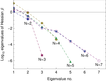
Figure 2: (Color online) Eigenvalues of the Hessian of $\beta_{int}$ evaluated at its maximum plotted for different numbers of free parameters $N$. The dashed lines are intended as a visual aid only.

For our optimized potentials, there is a substantial variation in the eigenvalues of the associated Hessian as may be seen from table 1 and fig. 2. Surprisingly, it appears that effectively only 2 parameters, those associated with the two large eigenvalues in the Hessian, need to be adjusted in order to achieve the maximum hyperpolarizability. There are, therefore, a very wide range of potentials near to the optimized one that have hyperpolarizabilities close to the maximum. This is consistent with the speculation of Kuzyk (2000) that only some aspects of the first few wavefunctions—specifically the ratios of energy differences and dipole matrix elements of the ground and first two excited states—significantly affect the objective function: relatively few parameters in the potential are required to adjust these three low-lying wavefunctions accurately enough to specify quantities derived from their integral such as dipole matrix elements. Variations of the potential where these wavefunctions are small, or rapid variations where they are large, have little effect on either energies or dipole matrix elements.

The eigenvectors of the Hessian allow us to determine what aspects of the optimized potential are pertinent to maximizing the hyperpolarizability. The variation in the potential $\Delta V^{j}(x)$ in the direction of the eigenvector associated with the $j$-th largest eigenvalue of the Hessian $h^{j}$ is

$$\Delta V^{j}(x)=\left.\frac{\partial V(x,\{P_{i}+\alpha v_{i}^{j}\})}{\partial\alpha}\right|_{\alpha=0}$$ (19)

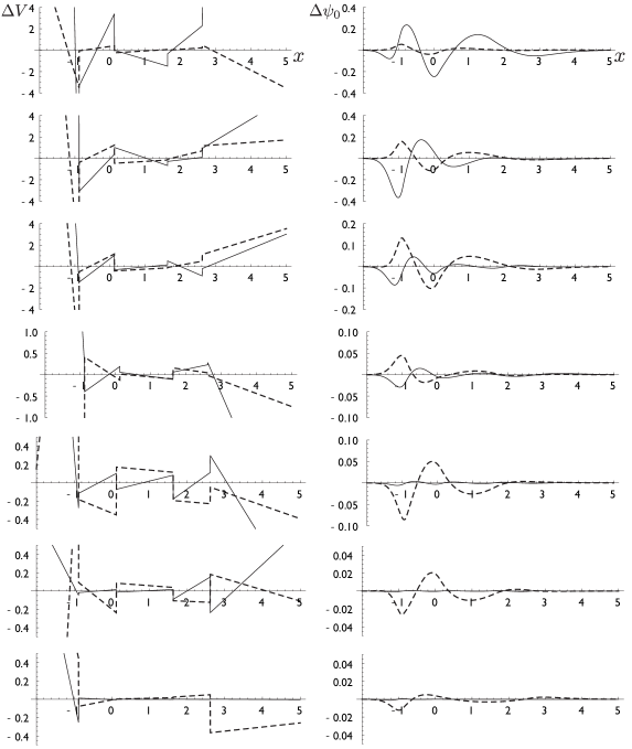
Figure 3: Variations of the potential and ground state wavefunction associated with eigenvectors of the Hessian matrix of $\beta_{int}$ evaluated at the maximum; these have been adjusted so that each variation simultaneously leaves $E_{1}-E_{0}=1$ and $\left\langle x\right\rangle=0$. The variations are plotted in descending order of eigenvalue. Each variation is calculated in two measures: the numerically natural measure (solid lines), and the measure of the ground state wavefunction (dashed lines).

where $v_{i}^{j}$ is the $i^{th}$ component of the $j$-th eigenvector. A small variation in the potential along this direction $V\rightarrow V+\alpha\Delta V^{j}$ will result in a corresponding change in the hyperpolarizability $\beta_{int}\rightarrow\beta_{int}+\frac{1}{2}h^{j}\alpha^{2}.$ The significance of such a variation is obscured by the fact that it typically contains some component that serves only to translate and rescale the energy and length. Since the hyperpolarizability is not affected at all by these operations, it is desirable to remove their associated components from the $\Delta V^{j}$. This may be achieved by rescaling $V$ and $x$ in the right hand side of (19) as a function of $\alpha$ to preserve the properties $\left\langle x\right\rangle=0$ and $E_{1}-E_{0}=1$ using (18). The resulting adjusted $\Delta V^{j}(x)$ no longer contain irrelevant rescalings or translations but appear to decrease in apparent size with decreasing eigenvalue (fig. 3), indicating that they are increasingly associated with either the irrelevant quantities $\left\langle x\right\rangle$, $E_{0}$ and $E_{1}-E_{0}$ or with changes where the wavefunctions are small. Unfortunately, those $\Delta V^{j}(x)$ associated with large eigenvalues do not seem to converge with increasing numbers of parameters and so reveal little about which features of the potential are truly important to the hyperpolarizability.

This suggests our parametrization of the potential could be improved, and also that a physically more relevant measure of “distance” between potentials is desirable. This measure is implicit in the process of finding the eigenvalues and eigenvectors of the Hessian; in the above analysis, it had the form

$$\left\|V_{1}-V_{2}\right\|^{2}=\left|P_{1}-P_{2}\right|^{2}$$ (20)

where the $P_{i}$ is the vector of parameters that specifies the $i$-th potential. While this idea of distance—referred to hereafter as the “numerically natural measure”—matters for the numerical process of finding the maximum, it is largely irrelevant to the design and synthesis of molecules that have large hyperpolarizabilities. To explore the possibility that the idea of distance between potentials matters for the interpretation of what matters for the potentials, we have constructed more physical measures of the distance between two potentials $V_{1}$ and $V_{2}$ as follows. First rescale each potential using (18) to set $\left\langle x\right\rangle=E_{0}=0$ and $E_{1}-E_{0}=1$, yielding scaled potentials $V_{1}^{s},$ $V_{2}^{s}$ for which the quantities irrelevant to the hyperpolarizability have been adjusted to have standard values. The measure is then

$$\left\|V_{1}^{s}-V_{2}^{s}\right\|_{k}^{2}=\int_{-\infty}^{\infty}\text{d}x\ \rho_{k}(x)\left|V_{1}^{s}-V_{2}^{s}\right|^{2}$$ (21)

where $\rho_{k}$ is a positive-definite weighting function. There are a wide variety of plausible possible choices for $\rho_{k}$: we used $\rho_{0}=\psi_{0}^{2}$ and $\rho_{1,0}=\psi_{0}^{2}+\psi_{1}^{2}$ where $\psi_{0}$ and $\psi_{1}$ are the normalized, scaled wavefunctions for the optimized potential as these measures serve to remove physically irrelevant differences between potentials, and are consistent with a priori expectations that only changes in the potential where low lying wavefunctions are large matter to the hyperpolarizability.

Eigenvalues of the Hessian were recalculated in each of these measures and are displayed in table 2. Clearly, the eigenvalues and eigenvectors of the Hessian are quite different for the different ways of measuring distances; unfortunately, this is particularly true for the eigenvectors that are associated with large eigenvalues of the hessian, i.e. those eigenvectors that tell us which changes to the potential do matter to the hyperpolarizability. Physically this is clear: changes that do not change the hyperpolarizability can be freely included in changes to eigenvectors with large eigenvalues if they do not also increase the distance. To examine this more precisely, consider the generalized eigenvalue problem with different measures of distances that may be written as

$$H_{ki}v_{i}^{j}=h^{j}M_{ki}v_{i}^{j}.$$ (22)

Here, in a given parametrization, $H_{kj}$ is the hessian of the objective function ($\beta_{int}$); $M_{kj}$ is the positive definite hessian of the measure of distance in the same parametrization; the $v_{i}^{j}$ are the eigenvectors and the $h^{j}$ are the eigenvalues. As only the eigenvectors and ratios of the eigenvalues are of interest, $\mathbf{M}$ can be chosen to have unit determinant. Some idea of the importance of the measure can be obtained by considering two nearly identical measures and calculating the changes in the eigenvalues and eigenvectors using perturbation theory in $\delta\mathbf{M}=\mathbf{M}_{1}-\mathbf{M}_{2}$. Let $h_{\alpha}^{j}$ and $\mathbf{v}_{\alpha}^{j}$ be the eigenvalues and eigenvectors within measure $\mathbf{M}_{\alpha}$ where eigenvectors are normalized by $\mathbf{v}_{\alpha}^{k}\mathbf{M}_{\alpha}\mathbf{v}_{\alpha}^{j}=\delta_{jk}$ and $\delta\mathbf{\bar{M}}=\left(\mathbf{M}_{1}\right)^{-1/2}\delta\mathbf{M}\left(\mathbf{M_{1}}\right)^{-1/2}$. Supposing the eigenvalues $h_{1}^{j}$ and eigenvectors $\mathbf{v}_{1}^{j}$ for the measure $\mathbf{M}_{1}$ are known and that $\delta\bar{\mathbf{M}}_{jk}=\mathbf{v}_{1}^{j}\delta\bar{\mathbf{M}}\mathbf{v}_{1}^{k}$ is small for $j\neq k$, the eigenvalues and eigenvectors $h_{2}^{j}$ and $\mathbf{v}_{2}^{j}$ in the second measure $\mathbf{M}_{2}$ may be found from a routine perturbation calculation:

$$h_{2}^{j}=h_{1}^{j}\left(\mathbf{1+v_{1}^{j}}\delta\bar{\mathbf{M}}\mathbf{v_{1}^{j}}\right)+\mathcal{O}\left(\delta\bar{\mathbf{M}}^{2}\right)$$ (23)

and

$$\mathbf{v}_{2}^{j}=\mathbf{v}_{1}^{j}+\sum_{j\neq k}\frac{\mathbf{v}_{1}^{k}h_{1}^{i}\left(\mathbf{v}_{1}^{k}\delta\mathbf{\bar{M}}_{1}\mathbf{v}_{1}^{j}\right)}{h_{1}^{j}-h_{1}^{k}}+\mathcal{O}\left(\delta\bar{\mathbf{M}}^{2}\right).$$ (24)

If $h_{1}^{j}\gg h_{1}^{k}$ any matrix element $\delta\bar{\mathbf{M}}_{jk}$ between these eigenvectors will result in a comparably sized change in the eigenvector: in other words, the contribution of an eigenvector that corresponds to a small eigenvalue to an eigenvector with a large eigenvalue is controlled largely by the measure and not by the nature of the hyperpolarizability. If, on the other hand, $h_{1}^{k}\ll h_{1}^{j}$, changes in the measure result in rather little change to the eigenvector. Unfortunately, the eigenvectors for which $h_{1}^{k}\gg h_{1}^{j}$ are the ones that ought to indicate which features of the optimized potential most affect the hyperpolarizability. For this reason, the question of which features of the potential do matter to $\beta_{int}$ is much harder to answer than the matter of what does not.

The changes in the scaled potential associated with each of the eigenvectors of the Hessian are displayed in fig. 3 with the numerically natural measure of eq. 20 and the measure of eq. (21) with $\rho_{0}=\psi_{0}^{2}$; also plotted are the corresponding changes in the ground and first excited state wavefunctions. Similar calculations for the other measures proposed produced similar behavior. Again, the superiority of a wavefunction description of the problem is clear from the fact that changes in the wavefunctions for the smaller eigenvalues are substantially smaller than those in the potential.

The scaled $h^{j}$ and $\Delta V^{j}(x)$ within a physically-motivated measure unambiguously identify the range of potentials close to the maximum. The breadth of this range with a variety of measures of distance suggests that the task of synthesizing near optimum chromophores or, at least, designing near-optimum potentials, may be easier than has been previously supposed; on the other hand it appears that while the parametrizations of the potential used previously have yielded useful estimates of the upper limit on the hyperpolarizability, they have also tended to obscure the underlying physics.

To further illustrate this, and to attempt to find a clear exposition of the important constraints for optimum hyperpolarizabilities, we calculated and display in table 1 two other physical quantities: the dipole transition matrix element from the ground to first excited state $x_{10}=\left\langle 1\left|x\right|0\right\rangle$ and the change in dipole moment between the ground and first excited state, $\Delta x_{10}=\left\langle 1\left|x\right|1\right\rangle-\left\langle 0\left|x\right|0\right\rangle$. Both of these have been previously identified(Zhou et al., 2006) from the sum-over-states formula as being important to optimizing $\beta$. Importantly, they can also be measured. It is apparent that both quantities converge with increasing number of parameters, $x_{10}$ to $\approxeq 55\%$ of the maximum possible value while less rapidly $\Delta x_{10}\approx 1.26$. Thus there appears to be, consistent with earlier work, a rather specific optimum value of $x_{10}$ and a less clear optimum choice for $\Delta x_{10}$. To further understand this we examined the derivatives of these parameters in the direction of each of the various eigenvectors of the hessian. These are given for $N=7$ parameters in table 2 and clearly diminish with the associated eigenvalue. The largest eigenvector with the largest eigenvalue seems quite strongly to constrain a linear combination of them, which is largely $\Delta x_{10}$ and the next largest eigenvalue constrains another combination that is largely $x_{10}$. The fact that $\Delta x_{10}$ is largely controlled by the largest eigenvalue is unusual given that $x_{10}$ converges more quickly than$\Delta x_{10}$. Nevertheless these quantities appear at first sight to offer a superior indication of how far a particular potential is from the optimum because deviations from the optimum alter them linearly, while the hyperpolarizability is only altered quadratically. It may be that combinations of these quantities, together with some other quantity presently unknown form a better indicator of the closeness of a potential to optimum, particularly for the second largest eigenvalue for the derivatives are not terribly large. Moreover, such ideas must be interpretted with care. It is, for example, physically clear that constructing a potential with a large barrier between the states that are important to the hyperpolarizability and a physically distant state precisely resonant with the first excited state will result in first and second excited states that are superpositions of the important excited state and this distant state. This will (of course) dramatically change $x_{10}$ and $\Delta x_{10}$ without significant effect on the hyperpolarizability. Nevertheless, for the single electron problem, and absent motions in special directions, these parameters, with the specific targets calculated herein seem reasonable heuristic, experimentally accessible measures of the distance of a physical system from the optimum.

IV Conclusions

We have determined that only 2 parameters are important in optimizing the zero frequency non-resonant hyperpolarizability of a single electron in a one-dimensional potential; these are associated with large eigenvalues of the Hessian of the hyperpolarizability, which are dramatically larger than the other eigenvalues with any of a number of physically motivated measures. Even with our careful optimization with few, appropriately chosen, parameters it is very difficult to distinguish the truly optimal potential from potentials with hyperpolarizabilities very close to the maximum. This is clearly a generic problem: there many, many potentials with virtually identical hyperpolarizabilities that will appear to most observers quite different from the true optimum potential. It seems relatively easy, particularly in light of the wide variety of such potentials obtained by others(Tripathy et al., 2004; Zhou et al., 2006, 2007), to design and produce systems whose potentials result in $\beta_{int}$ near the apparent maximum. However, the specific features of potentials that result in such hyperpolarizabilities are, almost in consequence, difficult to derive and explain. Our calculation is sufficient to reveal a wide variety of things that do not matter to the optimization, and to make clear that the optimum is more clearly expressed in terms of the wavefunction than the potential. While this is a significant improvement over prior works that take no special steps to understand which features of the potential are irrelevant, we were still unable to characterize to our satisfaction in a concise manner what does matter about optimum potentials. We believe that a quite different calculation—described in part below—would be required to determine this, though not uniquely as the question of relevance depends in part on specifying a measure of distance between potentials and these are motivated by a particular chemical or physical realization.

Given present results we are exploring other parametrizations of the potential: a judicious choice would only include variable features relevant to the maximization problem. The present work shows both that the optimized potentials become smoother with additional parameters and that rapid variations in the potential are irrelevant; this implies that the actual optimum potential is analytic. A promising approach is to expand the potential in a series of analytic functions such as Hermite polynomials and to maximize the hyperpolarizability with respect to the coefficients. Such a parametrization has some attractive features: If the optimal potential is analytic, the expansion should converge quickly with the higher order polynomials clearly corresponding to rapid variations in the potential that are known to be irrelevant. The following observations: that additional parameters make the potentials smoother; the eigenvalues of the hessian decrease rapidly; and that the eigenvectors somewhat resemble hermite polynomials with two added to the order; all suggest that the best potential is analytic as these characteristics would be expected for analytic potentials. Second, the numerically natural measure of distance between potentials induced by the weighting function of the Hermite polynomials is a physically reasonable one, since the weighting function itself resembles the electron’s probability density in the ground state. We therefore believe this parametrization ought to reveal more rigorous lower bounds on the maximum possible hyperpolarizability and a clearer description of the optimal potential. It is also expected, for numerically feasible optimizations, to appreciably decrease errors in the eigenvalues and eigenvectors of the hessian from purely numerical sources such as discretization and truncation. This, in turn, may make physical interpretation of these quantities, and specifically the parameters that most matter to the hyperpolarizability appreciably easier.

The consequences of our main results for the design of new non-linear chromophores are less obvious. Our clearest result is that numerically optimized potentials, such as those obtained in this work and elsewhere(Zhou et al., 2006, 2007), need very careful interpretation prior to use as design paradigms: both the parametrization and the optimization method are likely to result in appreciable “noise” that is without physical consequence. It seems remarkably difficult from our (or other) work to specify the range of nearly optimal potentials per se in any way that will matter to practical design. The $N=2$ and $N=7$ potentials of figure 1 differ by only slightly more than 1% in the optimum hyperpolarizability but appear physically dramatically different.

We have also demonstrated convincingly that the true upper bound on the hyperpolarizability of a single electron is appreciably below the bound derived from the dipole matrix element sum rules. With $n$ electrons, the maximum possible hyperpolarizability is predicted to be $n^{3/2}$ times that for a single electron. In fact this can be achieved in a system in which there are strong attractive interactions between the electrons that consequently move as a single quasi-particle in a potential similar that calculated above(Watkins and Kuzyk, 2011). This mechanism is likely only to be realizable in exotic systems due to the Coulomb repulsion of the electrons. A more practical lower limit on the bound is $n$ times the single electron maximum hyperpolarizability, which would correspond to the situation where the electrons are confined to non-interacting wells. Including repulsion, we speculate that the sum-rule bound increasingly overestimates the true bound with increasing numbers of electrons: two non-interacting electrons with opposite spins and Fermi statistics have twice, not $2^{3/2}$ times the upper bound on the susceptibility derived from the sum rules, while $n$ non-interacting bosons would have only $n$ rather than $n^{3/2}$ times the one particle bound. The fact that the bound for non-interacting electrons is smaller than that for attractive electrons suggests that it may also be a bound on electrons that repel each-other. Hence, it would appear that extant materials fall less spectacularly short of actual bounds than is presently claimed, although there is likely still substantial improvement possible in the hyperpolarizabilities.

Most importantly, it appears that surprisingly few parameters of the potential need to be adjusted to achieve close to optimum hyperpolarizability. Thus, while we do believe that significantly better chromophores can still in principle be made, it seems likely that careful, multidimensional optimization of potentials is not required to do this. Rather, only a few salient features need to be understood and adjusted appropriately. Beyond the obvious and well known ideas that the potential should be substantially, but not overly, asymmetric, and that the chromophore should absorb light well to the first excited state but only to some fraction of the sum-rule constraint, these features are as yet poorly understood.

No. of Parameters	Optimal $\beta_{int}$	$h_{min}/h_{max}$	$x_{10}$	$\Delta x_{10}$
1	0.659525	$0$
2	0.701633	$1.19\times 10^{-1}$
3	0.701923	$2.25\times 10^{-6}$	0.554604	1.354420
4	0.708764	$3.45\times 10^{-5}$	0.557740	1.268598
5	0.708928	$2.37\times 10^{-7}$	0.557752	1.269431
6	0.708836	$4.24\times 10^{-6}$	0.557762	1.269147
7	0.708951	$3.17\times 10^{-7}$	0.557763	1.269151

Table 1: For different numbers of parameters in the potential: (from the left) Optimized intrinsic hyperpolarizabilities for , together with the ratio of eigenvalues of the Hessian matrix of the intrinsic hyperpolarizability.

Eigenvalues of hessian			Derivatives of dipole matrix elements
Numerically natural Measure	$\rho_{0}$	$\rho_{10}$	$x_{10}^{\prime}$	$\Delta x_{10}^{\prime}$
$-3.28$	$-22.2$	$-8.10\times 10^{-1}$	$-3.21\times 10^{-1}$	$2.15$
$-3.14\times 10^{-1}$	$-4.70$	$-1.76\times 10^{-1}$	$-7.07\times 10^{-2}$	$5.35\times 10^{-3}$
$-1.09\times 10^{-2}$	$-1.15$	$-8.19\times 10^{-2}$	$-2.05\times 10^{-3}$	$4.96\times 10^{-3}$
$-4.83\times 10^{-3}$	$-2.47\times 10^{-1}$	$-3.16\times 10^{-2}$	$-1.47\times 10^{-3}$	$1.13\times 10^{-2}$
$-2.58\times 10^{-4}$	$-8.03\times 10^{-2}$	$-5.54\times 10^{-3}$	$-9.80\times 10^{-5}$	$3.91\times 10^{-4}$
$-1.66\times 10^{-5}$	$-4.65\times 10^{-3}$	$-3.03\times 10^{-3}$	$-1.23\times 10^{-5}$	$-7.71\times 10^{-6}$
$-1.04\times 10^{-6}$	$-3.12\times 10^{-4}$	$-2.02\times 10^{-4}$	$3.44\times 10^{-7}$	$-4.85\times 10^{-7}$

Table 2: Eigenvalues of Hessian for $N=7$ parameters in each of three measures: (from the left) the numerically natural measure induced by the parametrization; the measure $\rho_{0}=\left|\psi_{0}\right|^{2}$ and $\rho_{10}=\left|\psi_{0}\right|^{2}+\left|\psi_{1}\right|^{2}$. Derivatives of the dipole matrix in the direction of the eigenvector associated with each eigenvalue are also displayed.

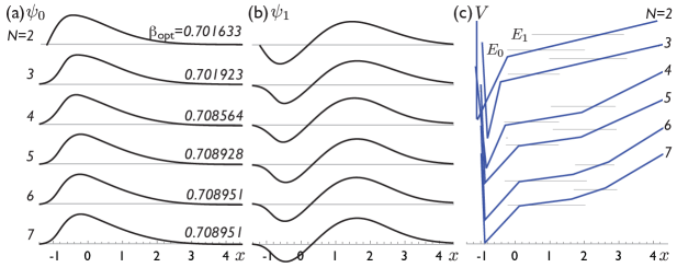
Figure 1: (Color online) (a) Ground and (b) first excited normalized wavefunctions corresponding to (c) optimized potentials for $N=2$ to $N=7$ parameters. Physically irrelevant positions and energies have been scaled out, consistent with eq. (18). The hyperpolarizabilities are noted in (a) and the ground and first excited energy levels are indicated in (c).

References

- Dalton et al. (1995) L. Dalton, A. Harper, R. Ghosn, W. Steier, M. Ziari, H. Fetterman, Y. Shi, R. Mustacich, A. Jen, and K. Shea, Chemistry of Materials 7, 1060 (1995).
- Kuzyk (2000) M. G. Kuzyk, Phys. Rev. Lett. 85, 1218 (2000).
- Tripathy et al. (2004) K. Tripathy, J. Moreno, M. Kuzyk, B. Coe, K. Clays, and A. Kelley, The Journal of chemical physics 121, 7932 (2004).
- Zhou et al. (2006) J. Zhou, M. Kuzyk, and D. Watkins, Optics letters 31, 2891 (2006).
- Zhou et al. (2007) J. Zhou, U. B. Szafruga, D. S. Watkins, and M. G. Kuzyk, Phys. Rev. A 76, 053831 (2007).
- Press et al. (2007) W. H. Press, S. A. Teukolsky, W. T. Vetterling, and B. P. Flannery, Numerical Recipes, 3rd Ed. (Cambridge University Press, 2007), chap. 10, pp. 387–448.
- Tarantola (2005) A. Tarantola, Inverse Problem Theory and Methods for Model Parameter Estimation (SIAM, 2005).
- Wiggers and Petschek (2007) G. Wiggers and R. Petschek, Optics letters 32, 942 (2007).
- Bretthorst (1988) G. L. Bretthorst, Bayesian Spectrum Analysis and Parameter Estimation. (Springer-Verlag, 1988), chap. 6, pp. 69–115.
- Watkins and Kuzyk (2011) D. S. Watkins and M. G. Kuzyk, J. Chem. Phys. 134, 094109 (2011).