Polylogs, thermodynamics and scaling functions of one-dimensional quantum many-body systems

Abstract

We demonstrate that the thermodynamics of one-dimensional Lieb-Liniger bosons can be accurately calculated in analytic fashion using the polylog function in the framework of the thermodynamic Bethe ansatz. The approach does away with the need to numerically solve the thermodynamic Bethe ansatz (Yang-Yang) equation. The expression for the equation of state allows the exploration of Tomonaga-Luttinger liquid physics and quantum criticality in an archetypical quantum system. In particular, the low-temperature phase diagram is obtained, along with the scaling functions for the density and compressibility. It has been shown recently by Guan and Ho (arXiv:1010.1301) that such scaling can be used to map out the criticality of ultracold fermionic atoms in experiments. We show here how to map out quantum criticality for Lieb-Liniger bosons. More generally the polylog function formalism can be applied to a wide range of Bethe ansatz integrable quantum many-body systems which are currently of theoretical and experimental interest, such as strongly interacting multi-component fermions, spinor bosons and mixtures of bosons and fermions.

and

1 Introduction

The one-dimensional Lieb-Liniger model [1] of interacting bosons is arguably the simplest Bethe ansatz integrable model [2, 3]. It is one of the most extensively studied many-body models of cold atoms. Experimental studies of cold bosonic atoms over a wide range of tunable interaction strength between atoms are in agreement with results obtained from the integrable model [8, 9, 10]. Moreover, the temperature dependence of this system provides a further experimental test [11] of integrable theory in the form of the Yang-Yang equation [12] in the weak coupling regime.

In principle, the Yang-Yang method gives exact results for the thermodynamic properties of integrable many-body systems at finite temperature [13]. However, depending on the particular model under investigation, the Yang-Yang method involves either a finite or an infinite number of coupled nonlinear integral equations, which hinders access to thermodynamic quantities from both the analytical and numerical points of view. It is a formidable task to extract exact low temperature results for many-body systems of this kind.

Here we further develop a polylog function method to derive the equation of state of homogeneous degenerate quantum gases of cold atoms in the framework of the TBA formalism. The polylog function method has been recently applied to the one-dimensional attractive Fermi gases of ultracold atoms [14, 15, 16, 17]. The thermodynamics and full phase diagrams can be calculated analytically via this approach. For example, for spin-1/2 attractive fermions, the universal Tomonaga-Luttinger liquid behaviour is readily identified from the pressure given in terms of polylog functions [14]. Here we investigate the thermodynamics of the Lieb-Liniger model for spinless bosons. The high precision of the equation of state obtained for strong interaction provides exact physical properties of this model at zero and finite temperatures. Following [18, 14], the universal Tomonaga-Luttinger liquid physics [19] follows with the help of Sommerfeld expansion in the low temperature limit. It was recently shown [17] that dynamical critical exponents and correlation exponents can be read off the universal scaling functions for thermodynamic properties of one-dimensional fermions. As we shall see below, the polylog function method is also accurate, simple and convenient in the study of thermodynamics and quantum criticality of one-dimensional bosons.

2 Thermodynamics of one-dimensional bosons

The Lieb-Liniger model [1] is described by the Hamiltonian

$${\cal H}=-\frac{\hbar^{2}}{2m}\sum_{i=1}^{N}\frac{\partial^{2}}{\partial x_{i}^{2}}+\,g_{\rm 1D}\sum_{1\leq i<j\leq N}\delta(x_{i}-x_{j})$$ (1)

in which $N$ spinless bosons, each of mass $m$, are constrained by periodic boundary conditions on a line of length $L$ and $g_{\rm 1D}={\hbar^{2}c}/{m}$ is an effective one-dimensional coupling constant with scattering strength $c$. We will be particularly interested in the low density case, i.e. the dimensionless parameter $\gamma=c/n$ is finitely strong, where $n=N/L$ is the linear density.

It was for this model that Yang and Yang [12] introduced the particle hole ensemble to describe the thermodynamics of the model in equilibrium, which is later called the thermodynamics Bethe ansatz (TBA), see [13]. In terms of the dressed energy $\epsilon(k)=T\ln(\rho^{h}(k)/\rho(k))$ defined with respect to the quasimomentum $k$ at finite temperature $T$, the Yang-Yang equation is

$$\epsilon(k)=\epsilon^{0}(k)-\mu-\frac{T}{2\pi}\int_{-\infty}^{\infty}dq\frac{2c}{c^{2}+(k-q)^{2}}\ln(1+{\mathrm{e}}^{-{\epsilon(q)}/{T}})$$ (2)

where $\mu$ is the chemical potential and $\epsilon^{0}(k)=\frac{\hbar^{2}}{2m}k^{2}$ is the bare dispersion. The dressed energy $\epsilon(k)$ plays the role of excitation energy measured from the energy level $\epsilon(k_{\rm F})=0$, where $k_{\rm F}$ is the Fermi-like momentum. The equilibrium states are described by the equilibrium particle and hole densities $\rho(k)$ and $\rho^{h}(k)$ of the charge degrees of freedom, which are subject to the equation

$$\rho(k)+\rho_{\rm h}(k)=\frac{1}{2\pi}+\frac{1}{2\pi}\int_{-\infty}^{\infty}dq\,\frac{2c\rho(q)}{c^{2}+(k-q)^{2}}.$$ (3)

The pressure $p(T)$ and free energy $F(T)$ are given in terms of the dressed energy by

$$p(T) = \frac{T}{2\pi}\int_{-\infty}^{\infty}dk\,\ln(1+\mathrm{e}^{-{\epsilon(k)}/{T}})$$ (4)

$$F(T) = \mu n-\frac{T}{2\pi}\int_{-\infty}^{\infty}dk\,\ln(1+\mathrm{e}^{-{\epsilon(k)}/{T}}).$$ (5)

It is important to observe that the log term in the Yang-Yang equation (2) vanishes exponentially for a large quasimomentum $k>k_{F}$ at low temperatures. For $T\rightarrow 0$, the ground state properties are determined by the so-called dressed energy equation

$$\epsilon(k) = k^{2}-\mu+\frac{c}{\pi}\int^{Q}_{-Q}dq\,\frac{\epsilon(k)}{c^{2}+(k-q)^{2}}.$$ (6)

The integration boundary $Q=k_{F}$ at zero temperature, i.e. $\epsilon(\pm Q)=0$. The pressure is given by

$$p=-\frac{1}{2\pi}\int^{Q}_{-Q}dk\,\epsilon(k).$$ (7)

This observation naturally suggests an expansion in powers of $1/c$ in the TBA (6), i.e.

$$\epsilon(k)=\epsilon^{0}(k)-\mu + \frac{c}{\pi}\frac{1}{c^{2}+k^{2}}\int^{Q}_{Q}dq\,\epsilon(q)$$ (8)

$$- \frac{c}{\pi}\int^{Q}_{-Q}dq\,\frac{\epsilon(q)}{(c^{2}+k^{2})^{2}}[-2kq+q^{2}]+O\left(\frac{1}{c^{4}}\right).$$

By way of a straightforward calculation with iterations through the pressure (7) and the condition $\epsilon(\pm Q)=0$, we find the relation

$$\epsilon(k) = \epsilon^{0}(k)-\mu-\frac{2pc}{c^{2}+k^{2}}+\frac{4\mu^{5/2}}{15\pi|c|^{3}}+O\left(\frac{1}{c^{4}}\right)$$ (9)

which gives

$$E\approx\frac{1}{3}n^{3}\pi^{2}\left(1-\frac{4}{\gamma}+\frac{12}{\gamma^{2}}+\frac{\left(\frac{32}{15}\pi^{2}-32\right)}{\gamma^{3}}\right)$$ (10)

as a highly accurate expansion for the ground state energy per unit length (in units of $\hbar^{2}/2m$).

For strong repulsion, Lieb-Liniger bosons behave like ideal particles obeying fractional statistics [20]. The gas reaches the Tonks-Girardeau regime with two-particle local correlation $g^{(2)}=\langle\Psi^{\dagger}(x)^{2}\Psi(x)^{2}\rangle/n^{2}\to 0$. Using the Hellmann-Feynman theorem, to leading orders the zero temperature two-particle local correlation follows as

$$g^{(2)}\approx\frac{4\pi^{2}}{3\gamma^{2}}\left(1-\frac{6}{\gamma}+\frac{1}{\gamma^{2}}\left(24-\frac{8}{5}\pi^{2}\right)\right)$$ (11)

which agrees with the result obtained from form factors of the Sine-Gordon model in the non-relativistic limit [21].

Turning to finite temperatures, the Yang-Yang equation can be expanded to $O(1/c^{4})$ as

$$\epsilon(k) = \epsilon^{0}(k)-\mu-\frac{2c\,p(T)}{c^{2}+k^{2}}+\frac{T}{2\pi(c^{2}+k^{2})^{2}}\int_{-\infty}^{\infty}dq\,q^{2}\ln(1+\mathrm{e}^{-{\epsilon(q)}/{T}})$$ (12)

$$\approx \epsilon^{0}(k)-\mu-\frac{2c\,p(T)}{c^{2}+k^{2}}-\frac{1}{2\sqrt{\pi}c^{3}}\frac{T^{\frac{5}{2}}}{\left(\frac{\hbar^{2}}{2m}\right)^{\frac{3}{2}}}\mathrm{Li}_{\frac{5}{2}}(-\mathrm{e}^{A_{0}/{T}})$$

where

$$A_{0} = \mu+\frac{2\,p(T)}{c}-\frac{4\mu^{5/2}}{15\pi|c|^{3}}$$ (13)

and

$$\mathrm{Li}_{n}(x)=\sum_{k=1}^{\infty}\frac{x^{k}}{k^{n}}$$ (14)

is the standard polylogarithm function [22]. From the dressed energy (12), the pressure at finite temperatures follows in terms of the polylog function as

$$p(T)\approx-\sqrt{\frac{m}{2\pi\hbar^{2}}}\,T^{\frac{3}{2}}\,\mathrm{Li}_{\frac{3}{2}}(-\mathrm{e}^{A/{T}})\left[1+\frac{1}{2c^{3}\sqrt{\pi}}\left(\frac{T}{\frac{\hbar^{2}}{2m}}\right)^{\frac{3}{2}}\mathrm{Li}_{\frac{3}{2}}(-\mathrm{e}^{A/{T}})\right]$$ (15)

where now

$$A = \mu+\frac{2\,p(T)}{c}+\frac{1}{2\sqrt{\pi}c^{3}}\frac{T^{\frac{5}{2}}}{\left(\frac{\hbar^{2}}{2m}\right)^{\frac{3}{2}}}\mathrm{Li}_{\frac{5}{2}}(-\mathrm{e}^{A_{0}/{T}}).$$ (16)

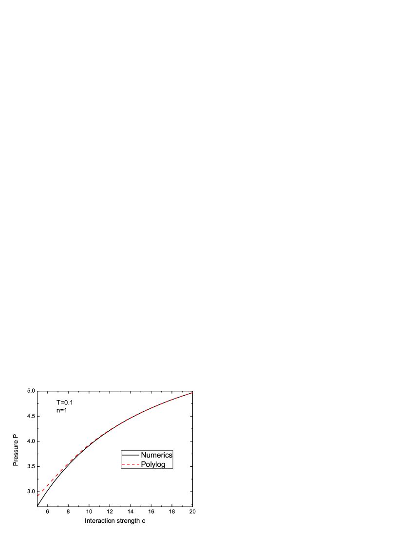
Figure 1: Pressure of Lieb-Liniger bosons vs interaction strength $c$. The curves show the comparison between results obtained using the polylog function and numerical solution of the integral equation.

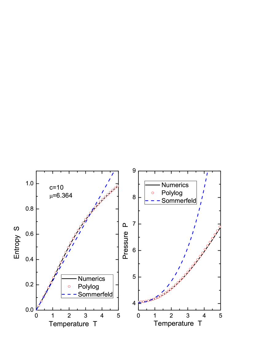
Figure 2: Finite temperature thermodynamics of Lieb-Liniger bosons. The curves show the comparison between the results obtained from numerics, the polylog function and Sommerfeld expansion for the entropy and the pressure.

The result (15) is essentially a high precision equation of state for Lieb-Liniger bosons. Figure 1 and Figure 2 show the excellent agreement between the analytic result (15) and the result obtained by numerically solving the TBA (2) at finite temperatures.

We touch briefly now on some physics of the model. For the grand canonical ensemble, the two-particle local correlation can be obtained from the free energy per particle $f=F(T)/n$ as $g^{(2)}=\frac{2m}{\hbar^{2}n^{2}}\left(\partial f/\partial\gamma\right)_{n,T}$ [23, 18]. The results also allow exploration of the crossover from the universal Luttinger liquid regime to the decoherent regime where the linear dispersion in the low-lying excitations is destroyed. Considering the low temperature limit, i.e. $T/(\frac{\hbar^{2}n^{2}}{2m})\ll 1$, the pressure per unit length with fixed $n$ is, to leading orders in $T$, given by

$$p(T)\approx p_{0}\left(1+\frac{\pi^{2}}{4}\left(1-\frac{8}{3\gamma}\right)\left(\frac{T}{\mu_{0}}\right)^{2}+\frac{\pi^{4}}{20}\left(1-\frac{16}{3\gamma}\right)\left(\frac{T}{\mu_{0}}\right)^{4}\right)$$ (17)

which follows directly by Sommerfeld expansion [18]. Here we have ignored higher order corrections than $1/c$ in the temperature-dependent terms. In the above result $p_{0}$ and $\mu_{0}$ are the pressure and chemical potential at zero temperature (in units of $\hbar^{2}/2m$)

$$p_{0} \approx \frac{2}{3}n^{3}\pi^{2}\left(1-\frac{6}{\gamma}+\frac{24}{\gamma^{2}}+\frac{\left(\frac{16}{3}\pi^{2}-80\right)}{\gamma^{3}}\right)$$ (18)

$$\mu_{0} \approx n^{2}\pi^{2}\left(1-\frac{16}{3\gamma}+\frac{20}{\gamma^{2}}+\left(\frac{64}{15}\pi^{2}-64\right)\frac{1}{\gamma^{3}}\right).$$ (19)

Moreover, to leading order, the free energy follows as

$$F(T)\approx E_{0}-\frac{\pi C(k_{B}T)^{2}}{6\hbar v_{c}}$$ (20)

where the central charge $C=1$, $E_{0}$ is the ground state energy (10) and $v_{c}\approx\frac{\hbar\pi^{2}n}{m}\left(1-\frac{4}{\gamma}+\frac{12}{\gamma^{2}}\right)$ is the sound velocity. The result (20) is as expected from conformal field theory arguments for a critical system, i.e. for a system with massless excitations. This implies that for temperatures below a crossover value $T^{*}$, the low-lying excitations have a linear relativistic dispersion relation, i.e. of the form $\omega(k)=v_{c}(k-k_{F})$. If the temperature exceeds this crossover value, the excitations involve free quasiparticles with nonrelativistic dispersion. This crossover temperature can be identified from the breakdown of linear temperature-dependent specific heat. Figure 2 indicates this universal crossover at a temperature $T^{*}\sim 1$ (in units of $k_{B}$) from a relativistic dispersion relation to a nonrelativistic dispersion.

For this simplest of models, the chemical potential drives a quantum phase transition from a vacuum phase into a Tomonaga-Luttinger liquid phase at zero temperature. We now further refine the equation of state to map out the universal low temperature quantum phase diagram.

3 Equation of state, scaling functions and phase diagram

For convenience in deriving the equation of state, we introduce an energy scale $\varepsilon_{0}=\hbar^{2}c^{2}/(2m)$. Equations (15) and (16) can then be written in terms of the dimensionless quantities $\tilde{\mu}=\mu/\varepsilon_{0}$ and $\tilde{T}=T/\varepsilon_{0}$ as

$$E := \frac{p}{\varepsilon_{0}c}\approx-\frac{\tilde{T}^{\frac{3}{2}}}{2\sqrt{\pi}}\mathrm{Li}_{\frac{3}{2}}(-\mathrm{e}^{{\tilde{A}}/{\tilde{T}}})\left[1+\frac{\tilde{T}^{\frac{3}{2}}}{2\sqrt{\pi}}\mathrm{Li}_{\frac{3}{2}}(-\mathrm{e}^{{\tilde{A}}/{\tilde{T}}})\right]$$ (21)

and

$$\tilde{A} = \tilde{\mu}-\frac{\tilde{T}^{\frac{3}{2}}}{\sqrt{\pi}}\mathrm{Li}_{\frac{3}{2}}(-\mathrm{e}^{{\tilde{A_{0}}}/{\tilde{T}}})+\frac{\tilde{T}^{\frac{5}{2}}}{2\sqrt{\pi}}\mathrm{Li}_{\frac{5}{2}}(-\mathrm{e}^{{\tilde{A_{0}}}/{\tilde{T}}})$$ (22)

with $\tilde{A}_{0}=\tilde{\mu}-\frac{\tilde{T}}{\sqrt{\pi}}\mathrm{Li}_{\frac{3}{2}}(-\mathrm{e}^{{\tilde{\mu}}/{\tilde{T}}})$. After a straightforward calculation, the density and compressibility are given by

$$n \approx -\frac{c\tilde{T}^{\frac{1}{2}}}{2\sqrt{\pi}}\mathrm{Li}_{\frac{1}{2}}(-\mathrm{e}^{{\tilde{A_{0}}}/{\tilde{T}}})\left[1-\frac{\tilde{T}^{\frac{1}{2}}}{\sqrt{\pi}}\mathrm{Li}_{\frac{1}{2}}(-\mathrm{e}^{{\tilde{A_{0}}}/{\tilde{T}}})+\frac{\tilde{T}}{\pi}\mathrm{Li}_{\frac{1}{2}}(-\mathrm{e}^{{\tilde{A_{0}}}/{\tilde{T}}})^{2}\right.$$ (23)

$$\left.-\frac{\tilde{T}^{\frac{3}{2}}}{\pi^{\frac{3}{2}}}\mathrm{Li}_{\frac{3}{2}}(-\mathrm{e}^{{\tilde{A_{0}}}/{\tilde{T}}})^{3}+\frac{3\tilde{T}^{\frac{3}{2}}}{2\sqrt{\pi}}\mathrm{Li}_{\frac{3}{2}}(-\mathrm{e}^{{\tilde{A_{0}}}/{\tilde{T}}})\right]$$

$$\kappa \approx -\frac{c}{2\varepsilon_{0}\sqrt{\pi}}\frac{1}{\sqrt{\tilde{T}}}\mathrm{Li}_{-\frac{1}{2}}(-\mathrm{e}^{{\tilde{A_{0}}}/{\tilde{T}}})\left[1-\frac{3\tilde{T}^{\frac{1}{2}}}{\sqrt{\pi}}\mathrm{Li}_{\frac{1}{2}}(-\mathrm{e}^{{\tilde{A_{0}}}/{\tilde{T}}})\right.$$ (24)

$$\left.+\frac{3\tilde{T}}{\pi}\mathrm{Li}_{\frac{1}{2}}(-\mathrm{e}^{{\tilde{A_{0}}}/{\tilde{T}}})\right].$$

In this model there exists one critical point at $\mu=\mu_{c}=0$, i.e. a quantum phase transition from the vacuum phase into a Tomonaga-Luttinger liquid occurs at $\mu=\mu_{c}$ at zero temperature. Near the critical point $\mu_{c}$ we find the density obeys the universal scaling form [24]

$$n(T,\mu)-n_{0}(T,\mu)\approx\tilde{T}^{\frac{d}{z}+1-\frac{1}{\nu z}}{\cal{F}}\left(\frac{\mu-\mu_{c}}{T^{\frac{1}{\nu z}}}\right)$$ (25)

for which the scaling function is ${\cal{F}}(x)=-\frac{c}{2\sqrt{\pi}}\mathrm{Li}_{\frac{1}{2}}(-\mathrm{e}^{x})$ for $T>|\mu-\mu_{c}|$. Here the background density in the vacuum is $n_{0}(T,\mu)=0$. For this model, we find that ${\frac{d}{z}+1-\frac{1}{\nu z}}=\frac{1}{2}$ and $\frac{1}{\nu z}=1$. Thus the critical exponent $z=2$ and the correlation length exponent $\nu=1/2$ with system dimension $d=1$ can all be read off the universal scaling form (25). Meanwhile, the compressibility satisfies the scaling form

$$\kappa(T,\mu)-\kappa_{0}(T,\mu)\approx\tilde{T}^{\frac{d}{z}+1-\frac{2}{\nu z}}{\cal{Q}}\left(\frac{\mu-\mu_{c}}{T}\right)$$ (26)

with ${\cal{Q}}(x)=-\frac{c}{2\varepsilon\sqrt{\pi}}\mathrm{Li}_{-\frac{1}{2}}(-\mathrm{e}^{x})$ and $\kappa_{0}(T,\mu)=0$.

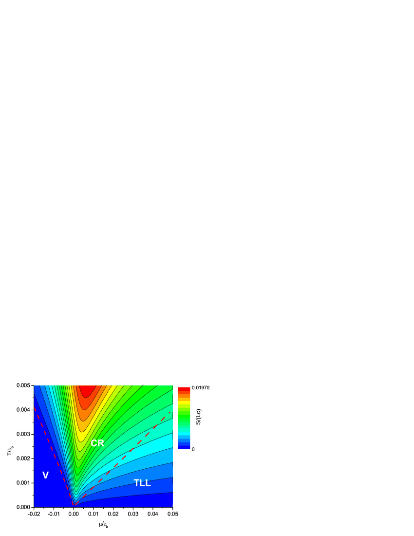
Figure 3: Quantum phase diagram of Lieb-Liniger bosons. The plot shows the entropy in the $T-\mu$ plane. The right red-dashed line denotes the crossover temperature separating the Tomonaga-Luttinger liquid (TLL) phase from the quantum critical regime (CR). The left red-dashed line separates the vacuum (V) from the quantum critical regime. For nonzero temperature, the vacuum produces particles with density $n\sim\frac{1}{\lambda}e^{-|\mu|/T}$ with thermal wavelength $\lambda=\sqrt{mk_{B}T/2\pi\hbar^{2}}$ which is much smaller than the inter-particle mean spacing. The vacuum can thus be taken as a semi-classical regime.

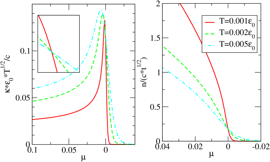
Figure 4: Quantum criticality is mapped out from the density and compressibility at low temperatures. The left panel shows the compressibility vs chemical potential at temperatures $T=0.001\varepsilon_{0}$, $T=0.003\varepsilon_{0}$ and $T=0.005\varepsilon_{0}$. The inset shows the universal scaling function near the critical potential $\mu_{c}=0$. The right panel shows intersecting density curves at the critical potential $\mu_{c}=0$.

The equation of state (21) has been used to plot the universal low temperature quantum phase diagram in Figure 3. The vacuum state and the Tomonaga-Luttinger liquid persist below the two cross-over temperatures. They both vanish at the quantum critical point, as described by the scaling functions. Following Zhou and Ho [24], the scaling functions for the density and compressibility can be used to map out the criticality of ultracold bosonic atoms in experiments. Figure 4 shows the detection of quantum criticality near $\mu_{c}=0$ using either the density or compressibility curves. We see clearly that such curves intersect at the critical potential $\mu_{c}$, indicative of scaling.

4 Concluding remarks

As highlighted in the Introduction, the motivation for the present work on one-dimensional bosons was the successful application of the polylog function method to the one-dimensional attractive Fermi gases [25, 26] of ultracold atoms up to order $1/c^{2}$ [14, 15]. Our key results are the equation of state (21) and the scaling forms (25) and (26) for the density and compressibility. The resulting low-temperature quantum phase diagram in Figure 3 is the simplest possible quantum criticality for quantum many-body systems.

In general, the polylog function method is widely applicable to one-dimensional many-body systems with quadratic bare dispersion or linear bare dispersion $\epsilon^{0}(k)$ in both attractive and repulsive regimes. The analytical polylog function method can thus play an important role in unifying the properties of attractive Fermi gases of ultracold atoms with higher symmetries. For example, the Yang-Yang method applied to the one-dimensional Fermi gas with attractive $\delta$-function interaction and internal spin degrees of freedom leads to equations which may be reformulated according to the charge bound states and spin strings characterizing spin fluctuations [15]. For strong attraction, the spin fluctuations that couple to non spin-neutral charge bound states are exponentially small and can be asymptotically calculated [14, 15]. Thus the low energy physics is dominated by density fluctuations among the charge bound states. The full phase diagrams and thermodynamics of the one-dimensional attractive Fermi gases can be analytically calculated with relative ease using this polylog function method. For example, for spin-1/2 attractive fermions, the universal Tomonaga-Luttinger liquid behaviour was identified from the pressure given in terms of polylog functions [14]. Here we further extend the results obtained using this approach.

Following the procedure described in the previous section, we obtain the pressure $p(T)=p^{b}(T)+p^{u}(T)$ from the TBA equations for spin-1/2 attractive fermions [13, 27]. The superscripts $b$ and $u$ denote bound pairs and excess fermions. For studying quantum criticality of 1D attractive Fermi gas [17], a high precision equation of state is highly desirable. To this end, the high order of corrections in $T$ and $1/|c|$ are retained as

$$p^{b}(T) = -\sqrt{\frac{m}{\pi\hbar^{2}}}\,T^{\frac{3}{2}}\,\mathrm{Li}_{\frac{3}{2}}(-\mathrm{e}^{{A_{b}}/T})\left[1-\frac{1}{4|c|^{3}\sqrt{2\pi}}\left(\frac{T}{\frac{\hbar^{2}}{2m}}\right)^{\frac{3}{2}}\mathrm{Li}_{\frac{3}{2}}(-\mathrm{e}^{{A_{b}}/T})\right.$$ (27)

$$\left.-\frac{2}{|c|^{3}\sqrt{\pi}}\left(\frac{T}{\frac{\hbar^{2}}{2m}}\right)^{\frac{3}{2}}\mathrm{Li}_{\frac{3}{2}}(-\mathrm{e}^{{A_{u}}/T})\right]+O\left(\frac{1}{c^{4}}\right)$$

$$p^{u}(T) = -\sqrt{\frac{m}{2\pi\hbar^{2}}}T^{\frac{3}{2}}\mathrm{Li}_{\frac{3}{2}}(-\mathrm{e}^{{A_{u}}/T})\left[1-\frac{4}{|c|^{3}\sqrt{2\pi}}\left(\frac{T}{\frac{\hbar^{2}}{2m}}\right)^{\frac{3}{2}}\mathrm{Li}_{\frac{3}{2}}(-\mathrm{e}^{{A_{b}}/T})\right]$$ (28)

$$+\,\,O\left(\frac{1}{c^{4}}\right).$$

Here we have defined the functions

$$A_{b} = 2\mu+\frac{c^{2}}{2}-\frac{p^{b}(T)}{|c|}-\frac{1}{4\sqrt{2\pi}|c|^{3}}\frac{T^{\frac{5}{2}}}{\left(\frac{\hbar^{2}}{2m}\right)^{\frac{3}{2}}}\mathrm{Li}_{\frac{5}{2}}(-\mathrm{e}^{{A_{0}^{b}}/{T}})$$

$$-\frac{4p^{u}(T)}{|c|}-\frac{4}{\sqrt{\pi}|c|^{3}}\frac{T^{\frac{5}{2}}}{\left(\frac{\hbar^{2}}{2m}\right)^{\frac{3}{2}}}\mathrm{Li}_{\frac{5}{2}}(-\mathrm{e}^{{A_{0}^{u}}/{T}})$$

$$A_{u} = \mu+\frac{H}{2}-\frac{2p^{b}(T)}{|c|}-\frac{2}{\sqrt{2\pi}|c|^{3}}\frac{T^{\frac{5}{2}}}{\left(\frac{\hbar^{2}}{2m}\right)^{\frac{3}{2}}}\mathrm{Li}_{\frac{5}{2}}(-\mathrm{e}^{{A_{0}^{b}}/{T}})+f_{s}$$ (29)

with

$$A_{0}^{b} = 2\mu+\frac{c^{2}}{2}-\frac{p^{b}(T)}{|c|}-\frac{4p^{u}(T)}{|c|}$$

$$A_{0}^{u} = \mu+\frac{H}{2}-\frac{2p^{b}(T)}{|c|}+f_{s}.$$ (30)

The spin string contributions to the thermal fluctuations in the physically interesting regime, $T\ll c^{2}$, $T\ll H$ and $|\gamma|\gg 1$, is given by $f_{s}=Te^{-\frac{H}{T}}e^{-\frac{2p^{u}(T)}{|c|T}}I_{0}\left(\frac{2p^{u}(T)}{|c|T}\right)$, in which $I_{0}$ is the standard Bessel function.

The above results may be immediately applied to obtain accurate thermodynamic quantities such as the magnetization, specific heat and density profiles in a trapping potential. One can compare with and fit the experimental results obtained recently for trapped one-dimensional spin-1/2 fermions at Rice University [28]. Indeed, the experimental results confirm the expected phase diagram [29, 30, 27, 31, 32, 33, 34, 35].

On the other hand, for one-dimensional Fermi gases with repulsive interaction [36, 37], we understand that antiferromagnetic effective spin-spin interaction directly couples to the charge degrees of freedom [38]. This triggers a spin-charge separated field theory of a Tomonaga-Luttinger liquid and an antiferromagnetic $SU(N)$ Heisenberg spin chain. With the help of Wiener-Hopf techniques and polylog functions, we also can obtain a high precision equation of state for such one-dimensional repulsive Fermi gases [39]. The application of this approach to the study of thermodynamics of other one-dimensional degenerate Bose and Fermi gases, such as the spinor Bose gases and to mixtures of bosons and fermions, is also relatively straight forward.

In general the equation of state provides essential insight into the thermodynamics of interacting many-body systems. Schemes have been proposed to directly measure the equation of state in experiments with ultracold atoms [40, 41]. Moreover, new schemes for mapping out the thermodynamics [42] and quantum criticality [24] of homogeneous systems by using the inhomogeneity of the trap can be directly applied to one-dimensional quantum many-body systems with a wide range of tunable interactions.

References

References

- [1] Lieb E H and Liniger W 1963 Phys. Rev. 130 1605
- [2] Korepin V E, Izergin A G and Bogoliubov N M 1993 Quantum Inverse Scattering Method and Correlation Functions (Cambridge University Press, Cambridge)
- [3] Batchelor M T 2007 Physics Today 60 36
- [4] Cazalilla M A 2004 J. Phys. B 37 S1
- [5] Petrov D S, Gangardt D M and Shlyapnikov G V 2004 J. Phys. IV France 116 5
- [6] Yurovsky V A, Olshanii M and Weiss D S 2008 Adv. Atom. Mole. Opt. Phys. 55 61
- [7] Pethick C J and Smith H 2008 Bose-Einstein Condensation in Dilute Gases (Cambridge University Press, Cambridge)
- [8] Kinoshita T, Wenger T and Weiss D S 2004 Science 305 1125
- [9] Kinoshita T, Wenger T and Weiss D S 2005 Phys. Rev. Lett. 95 190406
- [10] Haller E, Gustavsson M, Mark M J, Danzl J G, Hart R, Pupillo G and Nagerl H C 2009 Science 325 1224
- [11] van Amerongen A H, van Es JJP, Wicke P, Kheruntsyan K V and van Druten N J 2008 Phys. Rev. Lett. 100 090402 van Amerongen A H 2008 Annales de Physique 33 1
- [12] Yang C N and Yang C P 1969 J. Math. Phys. 10 1115
- [13] Takahashi M 1999 Thermodynamics of One-Dimensional Solvable Models (Cambridge University Press, Cambridge)
- [14] Zhao E, Guan X W, Liu W V, Batchelor M T and Oshikawa M 2009 Phys. Rev. Lett. 103 140404
- [15] Guan X W, Lee J Y, Batchelor M T, Yin X G and Chen S 2010 Phys. Rev. A 82 021606
- [16] He P, Yin X, Guan X W, Batchelor M T and Wang Y, arXiv:1009.2283
- [17] Guan X W and Ho T L, arXiv:1010.1301
- [18] Guan X W, Batchelor M T and Takahashi M 2007 Phys. Rev. A 76 043617
- [19] Giamarchi T 2004 Quantum Physics in One Dimension (Oxford University Press, Oxford)
- [20] Batchelor M T and Guan X W 2006 Phys. Rev. B 74 195121 Batchelor M T and Guan X W 2007 Laser Phys. Lett. 4 77
- [21] Kormos M, Mussardo G and Trombettoni A 2009 Phys Rev. Lett. 103 210404
- [22] Lewin L 1981 Polylogarithms and Associated Functions (North-Holland, New York)
- [23] Gangardt D M and Shlyapnikov G V 2003 Phys. Rev. Lett. 90 010401 Kheruntsyan K V, Gangardt D M, Drummond P D and Shlyapnikov G V 2003 Phys. Rev. Lett. 91 040403 Kheruntsyan K V, Gangardt D M, Drummond P D and Shlyapnikov G V 2005 Phys. Rev. A 71 053615
- [24] Zhou Q and Ho T L, arxiv:1006.1174
- [25] Yang C N 1967 Phys. Rev. Lett. 19 1312
- [26] Gaudin M 1967 Phys. Lett. A 24 55
- [27] Guan X W, Batchelor M T, Lee C and Bortz M 2007 Phys. Rev. B 76 085120
- [28] Liao Y et al., Nature 467, 567 (2010)
- [29] Orso G 2007 Phys. Rev. Lett. 98 070402
- [30] Hu H, Liu X J and Drummond P D 2007 Phys. Rev. Lett. 98 070403
- [31] Iida T and Wadati M 2008 J Phys. Soc. Jpn 77 024006
- [32] Casula M, Ceperley D M and Mueller E J 2008 Phys. Rev. A 78 033607
- [33] Kakashvili P and Bolech C J 2009 Phys. Rev. A 79 041603
- [34] Feiguin A E and Heidrich-Meisner F 2008 Phys. Rev. B 76 220508
- [35] Edge J M and Cooper N R 2009 Phys. Rev. Lett. 103 065301
- [36] Guan L, Chen S, Wang Y P and Ma Z-Q 2009 Phys. Rev. Lett. 102 160402
- [37] Ma Z-Q and Yang C N 2009 Chinese Phys. Lett. 26 120505 Yang C N 2009 Chinese Phys. Lett. 26 120504
- [38] Guan X W, Lee J Y and Batchelor M T 2008 Phys. Rev. A 78 023621
- [39] Lee J Y, Guan X-W, Sakai K and Batchelor M T, in preparation
- [40] Nascimbene S, Navon N, Jiang K J, Chevy F and Salomon C 2010 Nature 463 1057 Navon N, Nascimbene S, Chevy F, Salomon C 2010 Science 328 729
- [41] Horikoshi M, Nakajima S, Ueda M and Mukaiyama T 2010 Science 327 442
- [42] T L Ho and Q Zhou 2010 Nature Physics 6 131