Systematic Uncertainties in $B_{K}$ with Improved Staggered Fermions

Abstract:

We study three sources of error in our calculation of $B_{K}$ using HYP-smeared staggered fermions on the MILC asqtad lattices. These are (1) dependence on the light sea quark mass; (2) finite volume effects; and (3) the impact of an order of magnitude increase in the number of measurements. Our main results are (1) the dependence on the light sea-quark mass is weaker than expected by naive dimensional analysis, (2) including finite volume effects in SU(2) staggered chiral perturbation theory fits leads to a very small change in $B_{K}$, of size $\approx 0.1\%$, and (3) increasing the statistics on one of the coarse MILC lattices resolves a potential discrepancy with other coarse results.

1 Introduction

This paper is the third in a series of four proceedings describing our calculation of $B_{K}$ using improved staggered fermions. Here, we review some of the errors quoted in the error budgets for $B_{K}$ given in the companion proceedings [1] and [2]. In particular, we consider the following issues:

• The dependence of $B_{K}$ on the light sea quark mass $am_{\ell}$;

• Finite volume effects in the SU(2) analysis of $B_{K}$;

• The effect of increasing the number of measurements on the C4 ensemble.

For our notations for fits, and details of the ensembles we use, see Refs. [1, 2], as well as our recent long article [3].

2 Dependence of $B_{K}$ on light sea-quark masses

A year ago, we studied the light sea-quark mass dependence using five different “coarse” ($a\approx 0.12\;$fm) MILC ensembles, with results presented (using fits based on SU(2) staggered chiral perturbation theory [SChPT]) in Ref. [4]. In the intervening year, we have added a second sea-quark mass on the fine ($a\approx 0.09\;$fm) lattices (ensemble F2, with $am_{\ell}:am_{s}=0.0031:0.031$, i.e. with $m_{\ell}$ halved compared to ensemble F1), and also increased the statistics on one of the coarse ensembles (C4, with $am_{\ell}:am_{s}=0.007:0.05$). This allows us to solidify our understanding of the sea-quark mass dependence. This section summarizes the more extensive discussion given in Ref. [3].

Both SU(2) and SU(3) analyses allow us to extrapolate our results to the physical valence $d$ and $s$ masses, assuming that the corresponding ChPT is convergent. We use the SChPT fit forms to correct the chiral logarithms for the fact that the sea-quark masses differ from their physical values. Once these logarithmic corrections have been accounted for, the remaining dependence on sea quark masses is analytic, and given by

$$B_{K}=b_{0}+b_{1}(am_{\ell})+b_{2}(am_{s})+{\cal O}\left[(am)^{2}\right]\,.$$ (1)

Here $am_{\ell}$ and $am_{s}$ are the light and strange bare sea-quark masses, respectively. In SU(3) ChPT we have the additional relation $b_{2}=b_{1}/2$, while in SU(2) ChPT $b_{2}$ and $b_{1}$ are unrelated. In practice, we can only determine $b_{1}$, since, to date, all our ensembles have, for a given lattice spacing, the same value of $am_{s}$.

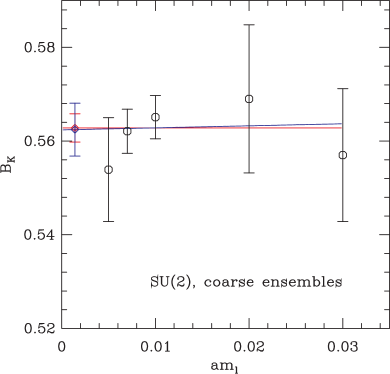
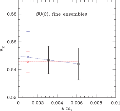
Figure 1: $B_{K}$ vs. $am_{\ell}$ for the MILC coarse ensembles (left) and for the MILC fine ensembles (right). These values are obtained using “4X3Y-NNLO” SU(2) fits [3, 1]. $B_{K}$ is obtained using one-loop matching and is evaluated at the scale $\mu=2$ GeV.

In Fig. 1, we show the dependence of $B_{K}$ (after extrapolation to physical valence quark masses) on $am_{\ell}$, for both coarse and fine lattices. The red and blue lines show, respectively, fits to a constant and a linear function. The fit parameters are given in Table 1. We see that the slope $b_{1}$ is consistent with zero, but has rather large errors. To compare the slopes at the two lattice spacings, we rewrite the expression (1) as

$$B_{K}=b_{0}\left[1+b^{\prime}_{1}(L_{P}/\Lambda_{\chi}^{2})\right]\,,$$ (2)

where $L_{P}$ is the mass-squared of the pion composed of light valence quarks (in physical units), and $\Lambda_{\chi}$ is the expansion scale of ChPT, which we take to be $1\;$GeV. Expressed this way, the slope coefficient $b^{\prime}_{1}$ should be the same for both lattice spacings, up to (presumably small) discretization errors. Furthermore, naive dimensional analysis suggests that $|b^{\prime}_{1}|={\cal O}(1)$. Values for $b^{\prime}_{1}$ are also given in the Table, and show that the magnitudes of the slopes are, in fact, considerably smaller than expected. This is not problematic, since a small value will occur some of the time. It is, however, serendipitous, since it reduces the uncertainty in the extrapolation to physical $am_{\ell}$.

$a$ (fm)	$b_{0}$	$b_{1}$	$b^{\prime}_{1}$
0.12	0.5624(64)	$+$0.04(58)	$+$0.005(74)
0.09	0.550(23)	$-$0.93(492)	$-$0.09(46)

Table 1: Parameters of the linear fits to SU(2) results shown in Fig. 1.

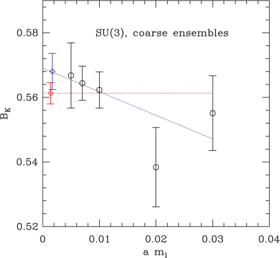
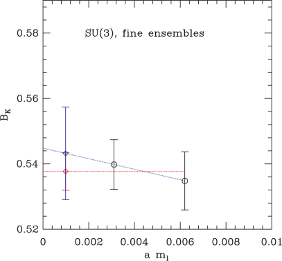
Figure 2: As in Fig. 1, but for the SU(3) analysis, using N-BB1 fits (see Ref. [2]).

The corresponding fits for the SU(3) SChPT analysis are shown in Fig. 2 with parameters given in Table 2. They give central values having somewhat larger magnitudes than the SU(2) fits, but they are still smaller than expected from naive dimensional analysis. Note that the slopes from the SU(2) and SU(3) fits need not be the same.

$a$ (fm)	$b_{0}$	$b_{1}$	$b^{\prime}_{1}$
0.12	0.5691(62)	$-$0.73(49)	$-$0.09(6)
0.09	0.5448(176)	$-$1.61(3.78)	$-$0.15(36)

Table 2: Parameters of the linear fits to SU(3) results shown in Fig. 2.

Since we find no evidence for a significant dependence on $m_{\ell}$, we assume, for our final value of $B_{K}$, that there is no such dependence, and do the continuum extrapolation using the $m_{\ell}/m_{s}=1/5$ lattices (including C3 and F1). We then correct for a possible dependence on $am_{\ell}$ by including in the error budgets a systematic error which is the difference in $B_{K}$ between the result on the C3 ensemble and that obtained using linear extrapolation to $am_{\ell}^{\rm phys}$ [3, 1, 2]. The error from an incorrect value of $am_{s}^{\rm phys}$ is estimated similarly.

3 Finite Volume Effects from SU(2) SChPT

Finite volume (FV) dependence is predicted by ChPT. At NLO, this dependence enters through corrections to the chiral logarithmic functions, as follows:

$$\ell(X) = X\left[\log(X/\mu_{\rm DR}^{2})+\delta^{\rm FV}_{1}(X)\right]\,,$$ (3)

$$\tilde{\ell}(X) = -\frac{d\ell(X)}{dX}=-\log(X/\mu_{\rm DR}^{2})-1+\delta^{\rm FV}_{3}(X)\,.$$ (4)

Here $X$ is the mass-squared of a pion, and $\mu_{\textrm{DR}}$ is the scale introduced by dimensional regularization. The FV corrections have the form of an image sum,

$$\delta^{\rm FV}_{1}(M^{2})=\frac{4}{ML}\sum_{\vec{n}\neq 0}\frac{K_{1}(|\vec{n}|ML)}{|\vec{n}|}\,,\qquad\delta^{\rm FV}_{3}(M^{2})=2\sum_{\vec{n}\neq 0}{K_{0}(|\vec{n}|ML)}\,,$$ (5)

where $L$ is the box size, and $\vec{n}$ labels the image position. For our geometries, sufficient accuracy is attained by keeping only spatial images.

In our previous work, including our long article [3], we have not included these finite volume corrections, due to the high computational cost of implementing them. Instead, we have shown that the expected size of these corrections is small compared to other errors [5]. This year, however, we have been able to do one-loop SU(2) SChPT fits including FV effects (keeping sufficient images that no approximation is made at double precision accuracy). To do so has required that we use GPUs. On a single core of the Intel i7 920 CPU (running at $\sim 0.5$ giga flops per core), a single FV fit to all ten MILC ensembles that we use takes about a week. Using an Nvidia GTX 480 GPU, by contrast, we have obtained a sustained performance of 67 giga flops (45% of the peak speed) [6]. Hence, using the GTX 480 GPU, it takes only about an hour to do the full SU(2) analysis for all the MILC ensembles. This is fast enough to carry out multiple fits, as is needed to estimate fitting errors.

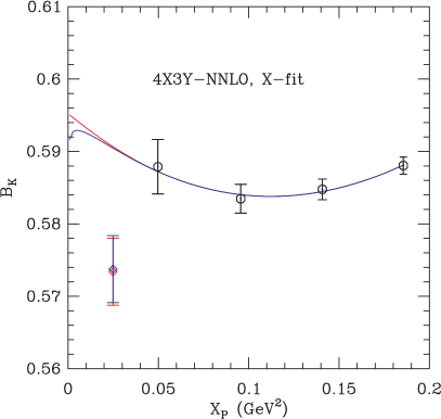
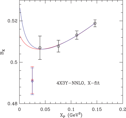
Figure 3: $B_{K}(\mu=1/a)$ (one-loop matched) versus $X_{P}$ (mass-squared of Goldstone-taste pion composed of quark and antiquark of mass $m_{x}$), including 4X-NNLO fits (explained in Ref. [3]). Ensembles are C3 (left, with $am_{y}=0.05$) and S1 (right, with $am_{y}=0.018$) ensembles. The red (blue) lines shows fit functions without (with) FV corrections included. See text for more details.

In Fig. 3, we compare the fits with and without FV corrections on a coarse (C3) and a superfine (S1–$a\approx 0.06\;$fm) ensemble. The red line shows the $V\rightarrow\infty$ fit, while the blue line includes FV corrections. The results of fits for $B_{K}$ are quoted in Table 3. These correspond to the red and blue points in the figures, and have been obtained by setting $m_{d}$ and $m_{\ell}$ to their physical values in the fit function, as well as removing taste splittings and setting $V\to\infty$ in the FV form. The impact of using the FV fit form is very small ($\sim 0.1\%$), as can be expected from the fact that the fit functions hardly differ for our pion masses. It is only for smaller values of $X_{P}$ that FV effects are visible. Note that the FV corrections have opposite signs on the two ensembles. This is due to a competition between two terms having different dependence on taste-splittings (and thus having different size on the two ensembles) [5].

ID	$B_{K}$	$B_{K}$(FV)
C3	0.5734(46)	0.5738(46)
S1	0.4914(65)	0.4908(65)

Table 3: Results for $B_{K}(\mu=1/a)$ with and without the finite volume corrections in the fit functions. The fits are those shown in Fig. 3.

It is well known that the one-loop prediction of FV effects gives only a semi-quantitative guide to their magnitude, since higher-loop effects can be important. For this reason, and to be conservative, we do not use the results just presented to estimate the FV systematic. Instead, we use the difference in $B_{K}$ obtained on the C3 and C3-2 ensembles (which have different spatial volumes), which leads to an error estimate of 0.85% [3].

4 Effect of Higher Statistics

Since last year, we added an additional 9 measurements on each lattice of the C4 ensemble, with the source timeslices chosen randomly, and different random seeds for the wall sources. In Ref. [7] we found that such additional measurements are, to good approximation, statistically independent. This new data allows us to resolve a small puzzle we had observed in last year’s data.

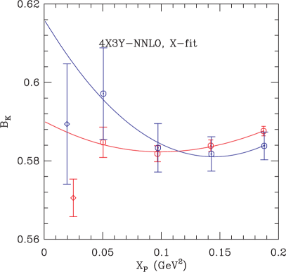
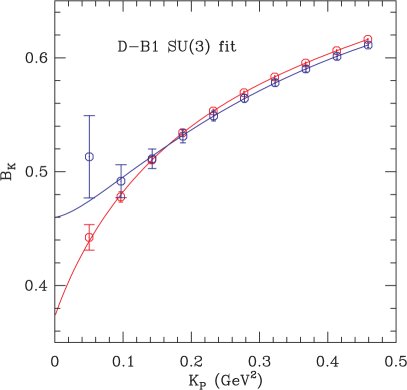
Figure 4: $B_{K}(\text{NDR},\mu=1/a)$ as a function of $X_{P}$ for the SU(2) analysis (left) and the SU(3) analysis (right) on the C4 ensemble. The fit types are 4X3Y-NNLO for SU(2) and D-B1 for SU(3) (see Ref. [3] for details). Blue points and fit correspond to 1 measurement/config while red data points and fit correspond to 10 measurements/config.

In Fig. 4, we compare the low and high statistics data. The data points have shifted in a way which is consistent with their original statistical uncertainties, but the result is a behavior, particularly at low $X_{P}$, more similar to that observed on other ensembles. Examples of the behavior on other ensembles are shown in Refs. [3, 1, 2].

This result illustrates the importance of obtaining small statistical errors, and also shows again how using multiple measurements on a single configuration is an efficient way of reducing errors.

5 Acknowledgments

C. Jung is supported by the US DOE under contract DE-AC02-98CH10886. The research of W. Lee is supported by the Creative Research Initiatives Program (3348-20090015) of the NRF grant funded by the Korean government (MEST). The work of S. Sharpe is supported in part by the US DOE grant no. DE-FG02-96ER40956. Computations were carried out in part on QCDOC computing facilities of the USQCD Collaboration at Brookhaven National Lab. The USQCD Collaboration are funded by the Office of Science of the U.S. Department of Energy.

References

- [1] Boram Yoon, et al., PoS (LATTICE 2010) 319; [arXiv:1010.4778].
- [2] Jangho Kim, et al., PoS (LATTICE 2010) 310; [arXiv:1010.4779].
- [3] Taegil Bae, et al., [arXiv:1008.5179].
- [4] Hyung-Jin Kim, et al. PoS (LATTICE 2009) 262; [arXiv:0910.5573].
- [5] Boram Yoon, et al. PoS (LATTICE 2009) 263; [arXiv:0910.5581].
- [6] Jangho Kim, et al., in preparation.
- [7] Jangho Kim, et al., PoS (LAT2009) 264; [arXiv:0910:5583].