Stars and (Furry) Black Holes in Lorentz Breaking Massive Gravity

Abstract

We study the exact spherically symmetric solutions in a class of Lorentz-breaking massive gravity theories, using the effective-theory approach where the graviton mass is generated by the interaction with a suitable set of Stückelberg fields. We find explicitly the exact black-hole solutions which generalizes the familiar Schwarzschild one, which shows a nonanalytic hair in the form of a powerlike term $r^{\gamma}$. For realistic self-gravitating bodies, we find interesting features, linked to the effective violation of the Gauss law: i) the total gravitational mass appearing in the standard $1/r$ term gets a multiplicative renormalization proportional to the area of the body itself; ii) the magnitude of the powerlike hairy correction is also linked to size of the body. The novel features can be ascribed to the presence of the Goldstones fluid turned on by matter inside the body; its equation of state approaching that of dark energy near the center. The Goldstones fluid also changes the matter equilibrium pressure, leading to an upper limit for the graviton mass, $m\lesssim 10^{-28\div 29}\,\text{eV}$, derived from the largest stable gravitational bound states in the Universe.

I Introduction

The question whether general relativity (GR) is an isolated theory is interesting from both the theoretical and phenomenological side. It is known that one can add to the Einstein-Hilbert Lagrangian a tower of higher order operators, starting with terms quadratic in the curvature, which produces corrections $\sim(E/M_{P})^{n}$, where $M_{P}$ is the Planck mass and $E$ is the typical energy of the process we are considering. Thus the predictions of GR at scales much larger then the Planck length $1/M_{P}$ are insensitive to them. Modifying GR at large distances is a totally different business. Besides its theoretical interest, the search for large-distance modified theories of gravity has been motivated by the evidence for cosmic acceleration and the consequent revival of the long-standing cosmological constant problem. The idea is to look for massivelike deformation of GR featuring a large-distance (infrared) modification of the Newtonian gravitational potential and a massive graviton.

It is instructive to start from perturbative gravity by considering a Lorentz-invariant theory of a massive spin-two field PF . The resulting theory is plagued by a number of diseases that make it probably unphysical. First, the modification of the Newtonian potentials is not continuous in the limit of very small graviton mass $m$ giving a large correction (25%) to the light deflection from the sun that is experimentally excluded DIS . The discontinuity manifests itself in the weak-field regime and a possible way to circumvent the problem at the full nonlinear order was proposed by Vainshtein in Vainshtein : if in the Fierz-Pauli theory (FP) the linearized approximation breaks down near the Sun the above mentioned discrepancy cannot be trusted anymore. He proposed using an improved perturbative expansion, which has a continuous limit for $m\to 0$. The relative solution is valid only up to a finite distance, and the question is then whether this solution can be extended up to infinity and matched with the Yukawa-like solution valid at large distances DAM . Recent evidences that this can indeed be achieved by means of a different weak coupling expansion have been addressed in deffayetlast . In addition, the FP theory is also problematic as an effective theory at the quantum level. Regarding FP as a gauge theory where the gauge symmetry is broken by a explicit mass term $m$, one would expect a cutoff $\Lambda_{2}\sim mg^{-1}=(mM_{P})^{1/2}$; however, the real cutoff is $\Lambda_{5}=(m^{4}M_{P})^{1/5}$ NGS much lower than $\Lambda_{2}$. A would-be Goldstone mode is responsible for the extreme UV sensitivity of the FP theory, which becomes totally unreliable in the absence of proper UV completion. These issues cast a shadow on the possibility of realizing a Lorentz-invariant theory of massive gravity VAIN .

It was recently noted that by allowing Lorentz-breaking mass terms for the graviton the resulting theory can be physically viable RUB , being free from pathologies such as ghosts or low strong coupling scales, and still lead to modified gravity. Since mass terms break the diffeomorphism invariance anyway, this possibility was analyzed mainly in a model-independent way, by reintroducing the Goldstone fields of the broken gauge invariance; and by studying their dynamics NGS ; DUB . For a recent review, see RUB-TIN . Lorentz-breaking massive gravity was also considered in the framework of bigravity USlett . In particular, we will be interested in a special phase of Lorentz-breaking massive gravity that has no propagating scalar perturbations around flat space. In this phase, the absence of dangerous instabilities survive in the curved spacetime, as shown in uscurved .

Besides its consistency, in order to be a viable theory massive gravity has to pass a number a tests. In GR the Schwarzschild solution is a benchmark and it is thus crucial to study the impact of a massive deformation on it. The main goal of this paper is to study both analytically and numerically the gravitational field produced in by a spherically symmetric body. The outline is the following. After the quick definition of the theory in the Stueckelberg approach in Sec. II, in Sec. III we find the generalized Schwarzschild solution for Lorentz-breaking massive gravity, and explicitly obtain the values of the two integration constants entering the exterior solution as a function of the mass and the size of the body. This result is obtained matching the exterior with the interior solutions for an object of constant density and using the nonstandard perturbative expansion. In Sec. IV we discuss the validity of perturbation theory and present a numerical analysis supporting our results also when gravity is strong inside the body. In section V we discuss some features of the black-hole solutions.

II IR Modified Theories

Infrared modified gravity theories with manifest diffeomorphism invariance can be realized by introducing a set of four Stückelberg fields $\Phi^{A}$ ($A=1,\ldots,4$) transforming under a diff $\delta x^{\mu}=\xi^{\mu}(x)$ as simple scalars. Then one can build new geometric objects, manifestly diff invariant, function of the metric field and the scalar fields, $g^{\mu\nu}\partial_{\mu}\Phi^{A}\partial_{\nu}\Phi^{B}$. A generic function of these quantities, when expanded around a background, can give rise to graviton mass terms. One can require that expanding around a Minkowski background the resulting mass terms are Lorentz-invariant. However, as discussed in the introduction, Lorentz invariant massive gravity is rather problematic; therefore, we relax this requirement and keep just rotational invariance in the theory. This approach is suited to describe a generic theory in an effective fashion, and a general action can be written as

$$\begin{split}&S=\int d^{4}x\sqrt{g}\left(M_{P}^{2}\,R+{\cal L}_{\text{matt}}\right)+S_{\text{gold}}\,,\\ &S_{\text{gold}}=\int d^{4}x\sqrt{g}\,m^{2}M_{P}^{2}\;{\cal F}({\cal X},V^{i},{\cal S}^{ij})\,,\end{split}$$ (1)

where ${\cal F}$ is a rotationally invariant potential, function of

$$\begin{split}&{\cal X}=-g^{\mu\nu}\partial_{\mu}\Phi^{0}\partial_{\nu}\Phi^{0}\,,\qquad V^{i}=-g^{\mu\nu}\partial_{\mu}\Phi^{i}\partial_{\nu}\Phi^{0}\,,\qquad{\cal S}^{ij}=-g^{\mu\nu}\partial_{\mu}\Phi^{i}\partial_{\nu}\Phi^{j}\,.\end{split}$$ (2)

The constant $m$ sets the graviton mass scale. Note that the breaking of Lorentz symmetry is directly built in the action; in Appendix A we discuss a different approach where the breaking is dynamical. Furthermore, additional symmetries of the Goldstone action can be used to single out a particular phase of massive gravity DUB . In particular taking

$${\cal F}\equiv{\cal F}({\cal X},W^{ij})\,,$$ (3)

where $W^{ij}={\cal S}^{ij}-{\cal X}^{-1}\,V^{i}\,V^{j}$, the Goldstone action is invariant under $\Phi^{i}\to\Phi^{i}+\xi^{i}(\phi^{0})$ and it turns out that, in a flat background, only the massive spin 2 tensor (2 elicities only) propagates DUB . The flat background admitted by the action (1) can be parametrized as

$$\bar{g}_{\mu\nu}=\eta_{\mu\nu}\,,\qquad\bar{\Phi}^{A}=(\,a\,t,\,b\,x^{i}\,)\,.$$ (4)

The background breaks boosts and preserves rotations, as can be seen by considering the additional effective background metric $\hbox{$\bar{g}_{2}$}_{\mu\nu}=\partial_{\mu}\bar{\Phi}^{A}\partial_{\nu}\bar{\Phi}^{B}\eta_{AB}=\text{diag}(-a^{2},\,b^{2},\,b^{2},\,b^{2}\,)$ (see Appendix A). The condition for the existence of the flat solution (4) is the vanishing of the background Goldstones energy momentum tensor [see (32) in Appendix B]. Due to rotational symmetry of the potential and of the effective $\hbox{$\bar{g}_{2}$}_{\mu\nu}$, this condition amounts to two independent equations that determine $a$, $b$ in terms of the parameters entering the potential. The background breaks Lorentz when $a\neq b$, but as noted above, the Lorentz breaking is built into the potential, not only in the background configuration. This is to be contrasted to theories with spontaneous breaking of Lorentz symmetry, as for instance in bigravity. Here, it is notable that for a generic potential function $\cal F$ a flat solution is always present, regardless of a cosmological constant term in the action.

Because of the nonzero background of the scalar fields, their fluctuations with respect to the background, $\pi^{A}=\Phi^{A}-\bar{\Phi}^{A}$; trasform under diffs as a Goldstone field, $\delta\pi^{A}=\xi^{\mu}(x)\partial\bar{\Phi}^{A}/\partial x^{\mu}$. A choice of coordinates setting the Goldstones fields $\pi^{A}=0$ fixes the gauge completely and is sometimes called the unitary gauge: all the dynamics is transferred to the metric.

III Spherically Symmetric Solutions

For the spherically symmetric case, one can always find a set of coordinates where the metric and the Goldstone fields have the following form

$$\begin{split}&ds^{2}=-dt^{2}\,J(r)+K(r)\,dr^{2}+r^{2}\,d\Omega^{2}\,,\\ &\Phi^{0}=a\,t+h(r)\,,\qquad\Phi^{i}=\frac{x^{i}}{r}\,\phi(r)\,.\end{split}$$ (5)

We will first derive the exact vacuum spherically symmetric solution describing the exterior part of the self-gravitating body, then we look for the interior part. Finally, the exterior and interior parts of the solution are matched to find the two integration constants, $M$ and $S$m which account for the gravitational mass of the body and the size of the powerlike term in the solution, one of the main novel features compared to GR.

III.1 Exterior, vacuum, exact solution

The Einstein equations in vacuum read

$$E^{\mu}_{\nu}=\frac{1}{2M_{P}^{2}}\,{T_{\text{g}}}^{\mu}_{\nu}\,,$$ (6)

where $E^{\mu}_{\nu}$ is the Einstein tensor and ${T_{\text{g}}}^{\mu}_{\nu}$ is the Goldstone energy momentum tensor (see Appendix B for details). Some general features can be established independently from the choice of ${\cal F}$. From the ansatz (5) it is clear that the Einstein tensor is diagonal and therefore also the Goldstone energy momentum must be diagonal: ${T_{\text{g}}}^{t}_{r}=0$. This gives

$$\frac{h^{\prime}}{K^{7}{\cal X}^{4}}\left[{\cal X}^{4}{\cal F}_{x}\,(JK)^{3}+{\cal X}^{2}{\cal F}_{1}\phi^{\prime 2}\,(JK)^{2}-2{\cal X}{\cal F}_{2}\,\phi^{\prime 4}\,JK+3{\cal F}_{3}\,\phi^{\prime 6}\right]=0\;$$ (7)

where ${\cal F}_{1}\,,{\cal F}_{2}\,,{\cal F}_{3}$ and ${\cal F}_{x}$ are defined in Appendix B, and ${\cal X}$ [see (40)] depends on $h^{\prime},J\,,K$. As a result, two branches arise: in the first the equation is solved by $h^{\prime}=0$; in the second, with $h^{\prime}\neq 0$, the term in square brackets of (7) can be solved for ${\cal X}$, or e.g. $\phi^{\prime}$. As noted already in the bigravity context, the first branch $h^{\prime}=0$, leads to equations that are very hard to solve analytically; therefore, we will concentrate on the second branch.

Then, by using the solution to ${T_{\text{g}}}^{t}_{r}=0$, one remarkably finds that ${T_{\text{g}}}^{t}_{t}-{T_{\text{g}}}^{r}_{r}=0$ independently from the potential. Therefore $E^{t}_{t}-E^{r}_{r}=0$, which implies that, as in GR,

$$K(r)=\frac{k_{0}}{J(r)}\,,$$ (8)

where $k_{0}$ is an integration constant. It not difficult to see that the remaining Einstein equations consist in 2 equations for 2 unknown functions $J(r)$, $h(r)$, that can in principle be solved.

To proceed further an explicit form for ${\cal F}$ must be provided. A quite general choice of ${\cal F}$, inspired to a class of bigravity theories studied in USsph , is

$$\begin{split}{\cal F}=&\ \bigg{[}\beta_{0}\,+\beta_{1}w_{-1}+\beta_{2}\left(w_{-1}^{2}-w_{-2}\right)+\beta_{3}\left(w_{-1}^{3}-3w_{-2}w_{-1}+2w_{-3}\right)\bigg{]}{\cal X}^{-1}+\\ &{}+\alpha_{0}+\alpha_{1}w_{1}+\alpha_{2}\left(w_{1}^{2}-w_{2}\right)+\alpha_{3}\left(w_{1}^{3}-3w_{2}w_{1}+2w_{3}\right)\,.\end{split}$$ (9)

where $w_{n}=\text{Tr}(W^{n})$. The truly remarkable feature of the class of potentials (9) is that the equation ${T_{\text{g}}}^{t}_{r}=0$ admits (still for nonvanishing $h^{\prime}$) a simple solution with

$$\phi=b\,r\,,\qquad\bar{\alpha}_{1}-4\bar{\alpha}_{2}+6\bar{\alpha}_{3}-\bar{\beta}_{0}+2\bar{\beta}_{1}-2\bar{\beta}_{2}=0\,,$$ (10)

where we defined $\bar{\alpha}_{n}=b^{-2n}\;\alpha_{n},\;\;\bar{\beta}_{n}=a^{-2}\;b^{2n}\;\beta_{n}$. The condition (10) should be regarded as an equation determining the Goldstone background $a$ (or $b$) in terms of the parameters of the potential. Using  (10) in the remaining equations, one obtains $h^{\prime 2}$ (see Appendix C) and finally the exact “black-hole” solution

$$J(r)=1-\frac{2GM}{r}+\Lambda^{2}r^{2}+2G\,S\,r^{\gamma}\,.$$ (11)

Here $M$, $S$ are two integration constants, while $G=1/16\pi M_{P}^{2}$ is the Newton constant and $\Lambda^{2}\equiv\frac{1}{6}m^{2}\left(12\bar{\alpha}_{3}-6\bar{\alpha}_{2}+\bar{\alpha}_{0}-3\bar{\beta}_{1}+12\bar{\beta}_{2}-18\bar{\beta}_{3}\right)$ is an effective “cosmological constant”. The exponent $\gamma$ is given by $\gamma=-2\left(2\bar{\alpha}_{2}-6\bar{\alpha}_{3}+\bar{\beta}_{1}-2\bar{\beta}_{2}\right)/(\bar{\alpha}_{1}-4\bar{\alpha}_{2}+6\bar{\alpha}_{3})$. This kind of solution was first found in USsph in the context of bigravity theories.

While the $1/r$ qnd $r^{2}$ terms are also present in the Schwarzschild-de Sitter solution, the last one represents a power-law correction to GR whose size is the new integration constant $S$. It does not contain the graviton mass scale, therefore this term is present in the exterior solution also in the limit of vanishing graviton mass. In other words the influence of the Goldstone modes survives even in the limit $m\to 0$.

Clearly, one can choose $b$ such that the effective cosmological constant vanishes, $\Lambda=0$. Then, for $\gamma<2$, the metric describes an asymptotically flat space, which is just the flat solution (4). The condition $\Lambda=0$ together with (10) are the two conditions for a flat solution determining $a$, $b$. The masses of fluctuations around flat space (see RUB ) are

$$m_{0}^{2}=\frac{3}{4}\left(\bar{\alpha}_{1}-\!4\bar{\alpha}_{2}+\!6\bar{\alpha}_{3}-\!\bar{\beta}_{1}+\!4\bar{\beta}_{2}-\!6\bar{\beta}_{3}\right)m^{2}\,,\quad m_{1}^{2}=0\,,\quad m_{2}^{2}=\frac{1}{2}\left(\bar{\alpha}_{1}-\!2\bar{\alpha}_{2}+\!\bar{\beta}_{1}-\!2\bar{\beta}_{2}\right)m^{2}\,,$$

$$m_{3}^{2}=\frac{1}{4}\left(\bar{\alpha}_{1}-\!6\bar{\alpha}_{3}-\!\bar{\beta}_{1}+\!8\bar{\beta}_{2}-\!18\bar{\beta}_{3}\right)m^{2}\,,\quad m_{4}^{2}=\frac{1}{4}\left(\bar{\alpha}_{1}-\!4\bar{\alpha}_{2}+\!6\bar{\alpha}_{3}-\!3\bar{\beta}_{1}+\!12\bar{\beta}_{2}-\!18\bar{\beta}_{3}\right)m^{2}\,$$ (12)

and since the mass of the (spin-two) graviton is $m_{2}^{2}$, the corresponding combination of coupling constants should be positive.

For $\gamma>-1$ the new term $S\,r^{\gamma}$ is dominant over the Newtonian term $M/r$, and accordingly the total gravitational energy of the solution, evaluated via the Komar mass integral, is infinite (see Appendix E). For $\gamma<-1$ instead the new term is subleading and the Komar energy is just the mass $M$. In the following we will limit ourselves to the case $\gamma<-1$.

If the metric represents the exterior geometry of a spherical “star”; the integration constants $M$ and $S$ can be computed in terms of the star parameters by matching the interior and the exterior solutions. This will be done in the next section.

Having the exact solution, it is interesting to discuss its behavior at large distances, in the case of asymptotically flat solutions, where it can be compared to the standard weak-field limit. Curiously, while $J$ (and $K$) are of the form $1+\epsilon$, with $\epsilon\sim 1/r$, the expression for $h^{\prime}$, shows that asymptotically $h\sim\sqrt{\epsilon}$. So, the solution does not fit in the standard democratic weak-field expansion, or in other words the standard weak-field expansion fails to capture the asymptotic behavior. The correct weak-field expansion is actually nondemocratic, where some fields are smaller than others. By a gauge transformation one can eliminate $h^{\prime}$ and turn on the $h_{0i}$ asymptotic components of the metric, that again are nondemocratic: $h_{0i}\sim h_{00}^{1/2}\sim h_{ij}^{1/2}$; this is analogous to the suggestion of Vainshtein for the Fierz-Pauli (Lorentz-invariant) theory, where in the vicinity of a source this expansion leads to a non analytic solution which is continuous in the graviton mass parameter $m\to 0$. In that case however, the non analytic solution is valid only up to a finite radius. The standard weak-field expansion, leading to the Yukawa falloff is in turn valid only at larger distances, but is discontinuous in $m$. It was the aim of deffayetlast to setup a nondemocratic expansion to match the large and small distance solutions. Here, it is remarkable that the above nondemocratic weak-field expansion is valid at all distances, as shown by the exact solution. In other words, the theory is always inside the Vainshtein radius.

III.2 Inside a -Star- and matching

Consider now a region where matter is present in the form of a perfect fluid with energy density $\rho$ and pressure $p$. Though a constant density fluid is not realistic, it represents a benchmark and in GR a great deal of interesting information on the possible stable gravitational bounded configuration can be derived. Different from GR, because of the presence of the Goldstone fields even for a constant density fluid the resulting Einstein equations are difficult to solve analytically (the full system of equations in presence of matter is given in Appendix C) and we have to rely on perturbation theory. Moreover, even the linearization procedure is not straightforward and one has to set up the nondemocratic weak-field expansion as discussed in the last section.

The starting point is the expansion in the weak-field $\epsilon$ parameter

$$J =1+\epsilon\,J^{(1)}+\cdots\,,\qquad \phi =b\,r+\epsilon\,\phi^{(1)}+\cdots\,,\qquad \rho =\epsilon\,\rho_{0}+\cdots\,,$$ (13)

$$K =1+\epsilon\,K^{(1)}+\cdots\,,\qquad h =\epsilon^{1/2}\,h^{(1)}+\cdots\,,\qquad p =\epsilon^{2}\,p^{(1)}+\cdots\,,$$

where $\rho_{0}$ is the constant density of the fluid. As discussed above, the different parametric size of $h$ is necessary to have a consistent expansion of the $t$-$r$ component of Einstein equations. Diff invariance of the matter action alone leads to the conservation of the matter EMT. Then, by expanding the metric, the pressure is of order $\epsilon^{2}$ and can be neglected at leading order.

The linearized solution contains four integration constants, two are set to zero by imposing regularity in $r=0$; the last two, together with $S$ and $M$ are determined by matching the interior and the exterior solution at the star radius $R$. For brevity, we only give here the solution for the case $\Lambda=0$ and $\gamma<0$. The final expressions are

$$J^{(1)} = \frac{GM_{0}}{R}\left[\xi^{2}-3+8\;\mu^{2}R^{2}\left(\frac{\;\xi^{2}}{\gamma^{2}-\gamma-2}-\frac{3\;\xi^{4}}{5(\gamma-3)(\gamma-4)}+\frac{6\;\xi^{1-\gamma}}{(\gamma+3)(2\gamma-1)(\gamma+1)(\gamma-2)}\right)\right];$$

$$\Delta^{(1)} = \frac{3\;G\;M_{0}}{R}\;(\xi^{2}-1);\qquad\phi^{(1)}=3\;b\;G\;M_{0}\left(\frac{\xi^{-\gamma}}{(\gamma+1)(\gamma+3)}+\frac{\xi^{3}}{2\;(\gamma+3)}-\frac{\xi}{2\;(\gamma+1)}\right),$$ (14)

where $M_{0}=\frac{4}{3}\,\pi\,R^{3}\,\rho_{0}$ is the bare mass of the star, $\xi\equiv r/R$ and finally $\Delta\equiv JK$ so that $\Delta^{(1)}=J^{(1)}+K^{(1)}$.

The parameter $\mu$ is a new important mass combination defined in terms of the masses around flat space, (12):

$$\mu^{2}\equiv m_{2}^{2}\,\frac{3\,m_{4}^{4}-m_{0}^{2}\,(m_{2}^{2}-3\,m_{3}^{2})}{m_{4}^{4}-m_{0}^{2}\,(m_{2}^{2}-m_{3}^{2})}.$$ (15)

Note that in general $\mu^{2}$ can be positive or negative. The function $h$ always appears as $h^{\prime 2}$ and is obtained in terms of $J^{(1)}$, $\phi^{(1)}$ and $\Delta^{(1)}$:

$${h^{\prime}}^{(1)\,2}=a^{2}\;\left(\frac{\gamma}{12\;m^{2}\;r^{2}}(\Delta^{(1)}-r\;J^{(1)^{\prime}}-J^{(1)})-J^{(1)}+\frac{(2-\gamma)}{r}\phi^{(1)}\,\right)$$ (16)

The last unknown, the pressure $p(r)$, is found by using the matter EMT conservation, and is expressed in terms of $J$ and an integration constant $p_{0}$, fixed uniquely when defining the radius $R$ as the point where $p(R)=0$. The pressure is of order $\epsilon^{2}$ but the ratio $\frac{p}{\rho_{0}}$ is of order one, therefore we have

$$\frac{p(r)}{\rho_{0}}=\left[\frac{J(R)}{J(r)}\right]^{1/2}\!\!-1\,\simeq\,\epsilon\,\frac{1}{2}\left[J^{(1)}(R)-J^{(1)}(r)\right]+O(\epsilon)^{2}\;.$$ (17)

By matching $J$, $J^{\prime}$ at $r=R$ with the exterior vacuum solution (11) (with $\Lambda=0$), we find the two exterior integration constants $M$ and $S$ in terms of the parameters of the star:

$$M=M_{0}\left[1-\frac{8\,\mu^{2}R^{2}}{5(\gamma+1)(\gamma-2)}\right],\qquad S=-\frac{24\;\mu^{2}\,M_{0}\;R^{1-\gamma}}{(\gamma-4)(\gamma+1)(2\gamma-1)(\gamma-2)}.$$ (18)

We thus find that the star acts as a source for the new term, $S\neq 0$, and that the bare mass $M_{0}$ is renormalized. For $\gamma<-1$, both $S$ and the mass shift $\Delta M=M-M_{0}$ have the same sign of $\mu^{2}$. Thus, for $\mu^{2}>0$ both corrections are positive, $M>M_{0}$ and $S>0$, while for $\mu^{2}<0$ both the corrections are negative and then $M<M_{0}$ and $S<0$.

The deviation from GR is measured by $S$ which scales as $R^{4-\gamma}$; as a result, bigger self-gravitating objects produce larger deviations. The difference between the gravitational mass seen by distant observers and the bare mass, $\Delta M=M-M_{0}$, can be traced back to the Goldstones’ energy density: we have, using the equation of motion (EOM),

$${T_{\text{g}}}_{tt}=-\,\frac{S(\gamma+1)}{4\pi}\,r^{\gamma-2}J(r)\,,$$ (19)

Thus in the exterior region the energy density of the Goldstones is positive (for $\mu^{2}>0$ and in the range $\gamma<-1$ we are considering). Moreover, having a regular solution in all the spacetime, the Komar energy can be computed as an integral of the total energy momentum tensor (matter + Goldstones) over a $t=const$ 3-ball of radius $\bar{r}$:

$$E_{\bar{r}}=-2\int_{t=const}\!d^{3}x\,\sqrt{h}\left(T_{\mu}^{\nu}-\frac{1}{2}T\,\delta_{\mu}^{\nu}\right)\zeta^{\mu}n_{\nu}=M_{0}+\Delta M+C_{1}\,m^{2}\,R^{5}\ \,\rho_{0}\,\left(\frac{\bar{r}}{R}\right)^{\gamma+1}\;;$$ (20)

with $C_{1}$ an irrelevant constant. For $\gamma<-1$, the energy is finite and equal to $M$ in the limit $\bar{r}\to\infty$.

   

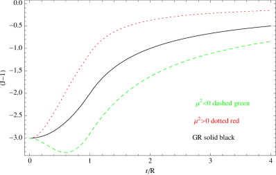
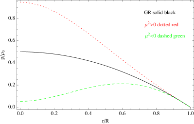
Figure 1: Plot, in the linear regime, of $J-1$ and $p/\rho_{0}$ in the case of massive gravity (III.2) and (17), both for $\mu^{2}$ positive and negative; also the standard GR case is shown for comparison. The numerical values used are : $\mu^{2}R^{2}=\pm 3.06$, $R_{s}/R=8.6\times 10^{-7}$ and $\gamma=-2.5$. The units are such that $GM_{0}/R=1$.

Since via $\mu^{2}$ both $S$ and $\Delta M$ are proportional to the graviton mass scale $m^{2}$, we conclude that for $m\to 0$ the deviations from GR disappear, both in the interior linearized solutions and in the exterior exact one:

$$J^{(1)}\to J^{(1)}_{\text{GR}}\,,\qquad K^{(1)}\to K^{(1)}_{\text{GR}}\qquad (r\leq R)$$ (21)

$$J\to J_{\text{GR}}\,,\qquad K\to K_{\text{GR}}\,,\qquad M\to M_{0}\,,\qquad S\to 0\,,\qquad (r\geq R)$$

where $GR$ indicates the corresponding expressions in general relativity. In the limit of vanishing graviton mass, GR is smoothly recovered even in the presence of the Goldstone fields $\phi$, $h$ that do not got to zero. Thus, there is no discontinuity for $m\to 0$ in the spherical star solution, and there is no sign of the Vainshtein scale $r_{V}$ that in the Pauli-Fierz theory invalidates standard perturbation theory at scales $r\lesssim r_{V}$. Here, the standard weak-field expansion is never valid, while the nondemocratic expansion is valid at all distances; in other words, $r_{V}=\infty$.

The above conclusions apply to realistic weak-field stars like the Sun. For the strong-field regime the inner star solution can be found numerically, and we discuss below some of its properties. Of course the present linearized solution coincides with the exact numerical one when the density is sufficiently low. In Fig. 1 the GR expression of $J$ and $K$ are compared with the ones found here for massive gravity.

III.3 Internal pressure and a bound on the graviton mass

The dimensionless parameter $\mu^{2}R^{2}$ plays a key role in determining the size of the deviations from GR. In particular it is interesting to investigate both the behavior of the internal pressure and of the total mass $M$, because their renormalization is sensitive to $\mu^{2}R^{2}$ and may turn negative when $\mu^{2}R^{2}$ is order one.

Clearly the stability of the matter system requires the pressure to be positive. One can see that it is enough to impose this condition at two regions, near the center and near the surface of the star. In particular, at the center of the star the requirement of positive pressure is

$$\frac{p(0)}{\rho_{0}}\simeq\frac{{GM_{0}}}{2R}\left[1-\frac{16\,\mu^{2}R^{2}\,(11-2\gamma)}{5\,(2\gamma-1)(\gamma-4)(\gamma-2)}\right]>0\,,$$ (22)

while to have positive pressure near the surface, where $p(R)=0$, its derivative has to be negative:

$$\frac{p^{\prime}(R)}{\rho_{0}}\simeq-\frac{{GM_{0}}}{2R}\left[1-\frac{16\,\mu^{2}R^{2}\,(\gamma+2)}{5\,(2\gamma-1)(\gamma-2)(\gamma-4)}\right]<0\,.$$ (23)

On the other hand, the requirement that the renormalized gravitational mass should be positive is

$$M=M_{0}\left[1-\frac{8\,\mu^{2}R^{2}}{5(\gamma+1)(\gamma-2)}\right]>0\,.$$ (24)

Thus, when $\gamma<-1$, we have $\delta p(0)\propto\mu^{2}$, $\delta p^{\prime}(R)\propto\mu^{2}\,\text{sign}(\gamma+2)$ and $\delta M\propto-\mu^{2}$. As a result, for positive $\mu^{2}$ the bound on $\mu^{2}$ comes from $p^{\prime}(R)$ (for $\gamma<-2$) and $M$, while for negative $\mu^{2}$ the bound comes from $p(0)$. This covers the whole range of $\mu^{2}$. In Fig. 2 we show the range of parameters spanned by such a requirements. The stronger bounds are due essentially to $M$ and $p(0)$.

Assuming no cancellations, or in other words that all mass scales in the potential are of the same order, the limit on $\mu^{2}$ can be interpreted as a limit on the graviton mass scale $m^{2}$.

The typical limit is therefore $m^{2}\sim|\mu^{2}|\leq{\cal O}(1)/R^{2}$; therefore, real stars with e.g. $R\sim 10^{5}\,$km, require $m<\times 10^{-11}\,$eV. Considering the Sun, for which $R\simeq 7\times 10^{5}\,$Km, and for which the central pressure may not deviate more than few percents from the standard value villante , we have $m<\times 10^{-13}\,$eV. However, since the limit does not depend on the mass of the body but only on its radius, it can be applied also in the extreme weak-field limit ($R\gg R_{s}$, see next section), for instance to very large and rarefied objects. In fact, larger objects give rise to stronger limits; for instance, the stability of the largest bound states in the Universe, $R\sim 1\div 10\,$Mpc, gives a limit $m<10^{-28\div 29}\,$eV.

Though the above considerations are strictly valid for a spherical symmetric and constant density body, we believe that for more realistic configuration the above limit can capture the correct order of magnitude. For other independent limits on graviton mass based on pulsar timing and CMB polarization effects see massgrav .

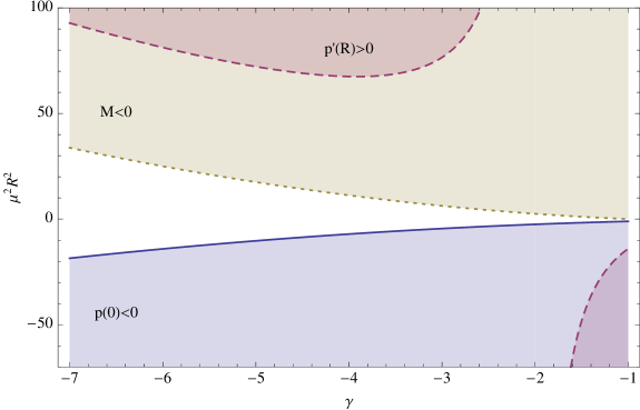
Figure 2: Excluded regions, in the ($\mu^{2}R^{2}$–$\gamma$) plane, from positivity of the pressure [$p(0)$ solid line, $p^{\prime}(R)$ dashed line] and of the renormalized mass $M$ (dotted line). The central white region is allowed.

Let us also comment that the positivity of the renormalized mass $M$ is not strictly required. In fact, a negative $M$ (and $\gamma<-1$) would lead to a repulsive gravity at large $r$ (only) while the body would still be in equilibrium, having positive pressure. Such and exotic behavior of the matter–Goldstones system may deserve further attention.

Regarding the validity of the bounds described above, an important discussion is in order. Clearly, the bounds hold, assuming that the description in terms of gravity coupled to a fluid is valid at the scales of interest, e.g. galaxies or a cluster of galaxies. This issue is far from being trivial, since, e.g. in standard gravity, the application of the same theory at different scales is guaranteed only in the Newtonian limit by the linearity of the field equations. In nonlinear cases, like for strong field or in the cosmological evolution, the description in terms of averaged quantities is expected to need effective corrections, which are under active discussion (see e.g. average ). In the present theory, two comments can be made. First, the description of matter in terms of a gravitationally bound fluid is appropriate, because the typical interparticle distance is small with respect to the size of the body and to the range of the gravitational force, which we recall is always infinite[(the Newtonian term in Eq. (11)]. On the other hand, the averaging of the gravitational field equations is non trivial, because, as it is shown by Eq. (16), one of the Goldstone fields enters quadratically, $(h^{\prime})^{2}$. (accordingly, $h^{\prime}$ is of order $\sqrt{\epsilon}\sim 1/\sqrt{r}$ in the exact and semilinearized approach that we described). Because of this nonlinearity, one expects a violation of superposition of multiple solutions, even in weak-field regime Notice that this nonsuperposition has to arise also in the Lorentz-invariant version of massive gravity Vainshtein , where one of the fields, essentially $h^{\prime}$, enters quadratically and has a $1/\sqrt{r}$ falloff. We expect in fact this to be a generic phenomenon in massive gravity. What we can conclude is that if one assumes the present description of gravity to be applicable at some scale of interest, i.e. galaxy clusters, then stability of the system leads to the strong bound derived above.

IV Perturbation theory and Beyond

IV.1 Validity of Perturbation Theory

Let us now study the validity of perturbation theory in both the inner and outer region of the -star’-. In GR it is well known that perturbation theory can be used when $r/R_{s}\gg 1$, with $R_{s}=2GM_{0}$ the Schwarzschild radius. By inspection of the expression for the metric perturbation (14) inside the body it is clear that perturbation theory is valid when

$$R_{s}\ll R\,,\qquad\mu^{2}\,R_{s}\,R\ll 1\,.$$ (25)

In this section we use $\mu^{2}$ as $|\mu^{2}|$ always positive defined.

If we were unable to find an exact solution in the outer region we could have set up the very same nondemocratic perturbation scheme as in (13). In fact, solving the linearized equation we find

$$J^{(1)}=\frac{j_{1}}{r}+f_{1}\,r^{2}+j_{2}\,r^{\gamma}+f_{2}\,r^{1-\gamma}\,,\qquad K^{(1)}=-J^{(1)}\,,\qquad\phi^{(1)}=f_{1}\,r+f_{2}r^{-\gamma}\,;$$ (26)

where $j_{1,2}$ and $f_{1,2}$ are integration constants. When $\gamma<-1$, to be in the weak-field regime at large $r$ we have to set $f_{1}=f_{2}=0$, and we get the linearized version of the exterior solution. The expansion is valid when $j_{1}/r\ll 1$ and $j_{2}\,r^{\gamma}\ll 1$. Using the values (18) of $j_{1}$ and $j_{2}$ obtained from the matching with the interior solution, we get, for $r>R$, the conditions

$$r\gg R_{s}\,,\qquad r\gg\,R\,\,(\mu^{2}\,R_{s}\,R)^{1/|\gamma|}\,.$$ (27)

The first condition makes sure that we are away from the would-be horizon at $r_{G}$ and it is trivially satisfied in the presence of the interior part of the solution with $R>R_{s}$. Notice that in the range $\gamma<-1$, thanks to (25), also the second condition is automatically satisfied. Then, once perturbation theory is valid in the interior of the body it can also be used in the exterior part. When (25) is not satisfied, the determination of $S$ and $M$ cannot be done using perturbation theory. In this case one can solve numerically the equations in the interior part and match the numerical solution with analytical exact solution that we have found in vacuum.

It is worth stressing that even within the perturbative region (25) sizable corrections to the gravitational mass $M$ are possible. This is the case for large bodies with $R$ of order ${\cal O}(1)/\mu$ . In this case, the second relation of (25) becomes equivalent to the first one $R_{s}\ll R$, but the dimensionless quantity $\mu^{2}\,R^{2}$ appearing in $M$ can be sizable.

IV.2 Beyond Perturbation Theory

When the equations in (25) are violated, perturbation theory cannot be trusted anymore and one needs a different tool to see what happens in this regime. We have solved numerically the Einstein equations in the interior, still modeling matter as perfect incompressible fluid. Figure 3 shows $M$ and $S$ computed numerically for different values of the graviton mass and matter density. From the numerical analysis it is clear that the linearized matching captures the basic features of the geometry. Indeed, the difference with the linear predictions are rather small and below 15 % for $R_{s}/R\sim 0.5$.

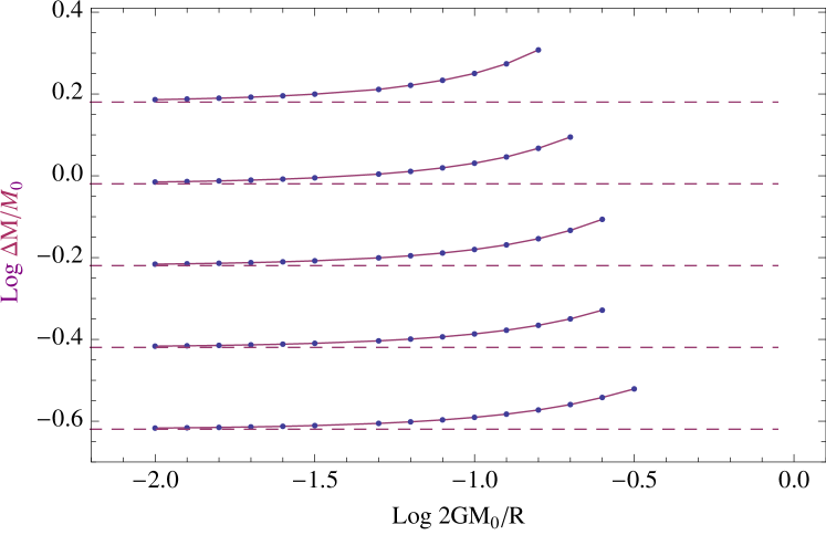
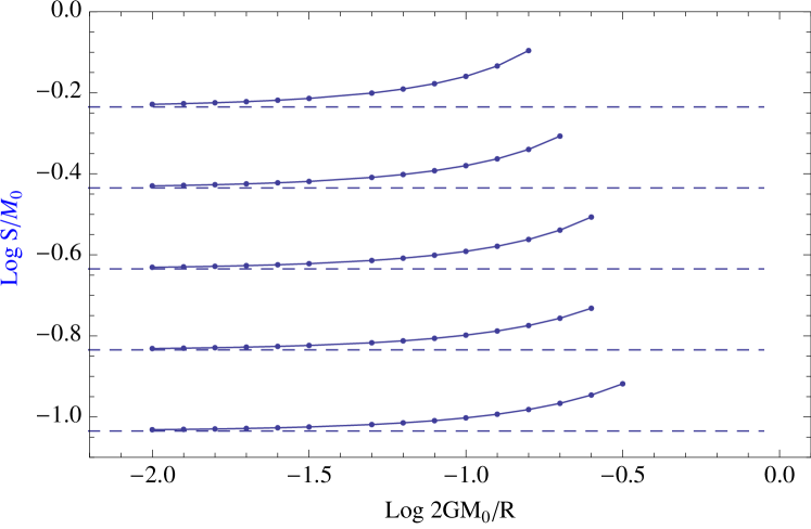
Figure 3: Numerical results for $\Delta M=M-M_{0}$ (left) and $S$ (right) for different values of the matter density and of the graviton mass scale $\mu^{2}R^{2}=0.1,\ldots,1$ (lower to upper). The dashed lines correspond to the perturbative values; (18).

The numerical analysis confirms the absence of a discontinuity for vanishing graviton mass, as discussed above in the perturbative analysis [see (21)]. Lowering the values of $m$, while keeping fixed the density, we have found a behavior compatible with $S,\Delta M\to 0$, up to the moderate strong-field regime $R_{s}/R\sim 0.3$, and down to small graviton mass scale $mR\sim 10^{-4}$. The numerical analysis thus shows no sign of discontinuity in $m$.

The remarkable feature that larger bodies gravitate more survives at the nonperturbative level. The relative mass renormalization for a body of size $R\sim m^{-1}$ is large, $\Delta M/M_{0}\sim 1$. In Fig. 4 we extend the perturbative bound on the dimensionless combination $mR$ to the region where $R_{s}/R\sim 0.5$. The result is that toward a strong field, the Goldstone pressure becomes even more negative, pushing the limit on $mR$ even lower. Of course real heavy objects are always small, therefore the bound given above in Sec. III.3 for large weak-field objects is more stringent.

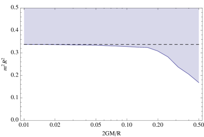
Figure 4: Numerical exclusion plot of the graviton mass [from $p(0)>0$] toward the strong field. Here $\gamma$ is fixed and the perturbative limit from (22) is $\mu^{2}R^{2}<0.338$ (dashed line).

Finally, the fact that the central pressure receives a negative contribution from the Goldstone EMT; points to the possibility of relaxing the Chandrasekar bounds on the density which, we recall, arise in the strong-field regime when the central pressure diverges. There may be then a regime where the negative pressure of the Goldstones balances the high gravitational force, allowing for compact heavy objects with arbitrarily high mass. We could not reach this regime with our numerical analysis that becomes arduously difficult near the origin, when going beyond $R_{s}/R\sim 0.5$.

V Massive Gravity Black Holes with Hair

It is known that in GR the gravitational hydrostatic equilibrium cannot be attained for arbitrary $M$ and $R$, for instance a body of uniform density cannot have a mass larger than $M=4R/9$, and for a fixed radius, this limit applies to any equation of state. The limit is crucial, because when a star in its late evolutionary state has exceeded it, the gravitational collapse cannot be stopped and a black hole is expected to form.

In GR, the spherically symmetric (uncharged) black holes are parametrized by its mass $M$. In massive gravity, as we showed, they are parametrized by an additional parameter, $S$. Suppose then that the late stage of the evolution of a star is described by our exterior metric

$$ds^{2}=-J\,dt^{2}+K\,dr^{2}+r^{2}d\Omega^{2}\,,\qquad J=1-\frac{2GM}{r}+2GS\,r^{\gamma}=K^{-1}\,.$$ (28)

and for definiteness let us consider here the case with $M>0$. In general, the hyper-surface at $r=r_{H}$ where $J(r_{H})=0$ is a Killing horizon: at $r=r_{H}$ the norm of the timelike Killing vector $\partial/\partial t$ vanishes. If $J$ is never vanishing the singularity at $r=0$ is naked. This happens when $S$ is large and positive, $S\geq\frac{R_{s}^{|\gamma|}}{4G}$. When $S$ is negative $J$ has a single zero. Finally, there is a range of $S$ where $J$ has two zeroes or one, namely $0<S<\frac{R_{s}^{|\gamma|}}{4G}$. When two zeros of $J$ are present, typically the outer Killing horizon is an event horizon for the black hole. For instance, in the case $\gamma=-2$ the solution is formally the same of a Reisser-Nordstrom black hole. To disentangle the causal structure in the general case one has to try to maximally extend the solution found using a set of Schwarzschild-like coordinates that fail at the outer Killing horizon. We leave the detailed study for a future work.

An other evident feature of the black-hole solution (28) is that it is one of the few examples of exact black holes with hairs in four spacetime dimensions. Their existence is considered to be forbidden in various classes of theories, by “no-hair” theorems (starting from bekenstein ). These are usually based on the positivity of suitable volume integrals, and often rely on linearity of the field equations. For instance, a no-hair theorem for the Fierz-Pauli massive gravity was described already in bekensteinPF , where only the quadratic FP mass terms were included. As we have proven here, the full theory of nonlinearly interacting massive gravity on the contrary generates hairs, extending in the asymptotic region. These hairs, depending on the value of $\gamma$, can even dominate over the Newtonian term, and even make the solution not asymptotically flat ($\gamma\geq 2$), leading to a type of furry black hole.

The situation is thus similar to known cases of black holes with hairs in non-Abelian gauge theories (colored black holes). However, classical non-Abelian fields are actually not observable (due to confinement). The example provided here would be the first example of classical hairs from nonlinearly interacting fields.

In the literature there are a number of no-hair theorems which also consider specifically the presence of extra scalar fields (see for instance Her ) that, in principle apply to our case. However, “technical” simplifying assumptions on the form of scalar field Lagrangian are often made, rendering the above results not directly relevant to our nonminimally coupled and interacting set of scalars.

We stress that the fields associated with these hairs (both the metric and the Goldstones) are nonsingular in all the space, except at the origin, where in any case the singularity is expected. Also, in the smooth star solution that we constructed, these fields are never singular.

Clearly, whether hairs will actually be present in real black holes, i.e. whether $S$ will be nonzero at the final stage of collapse, will depend on the collapse history, which is surely worth of a separate study. For instance, the fact that in the star solution the corrections to GR are proportional to the star’s surface area, i.e. $\Delta M,S\sim R^{2}$ (but only in weak-field) may lead one to think that $S\to 0$ during collapse. Or on the contrary one may think that the collapse itself may be stopped or reversed leading to a final “remnant” with a non-zero $S$. We stress in fact that the Birkhoff theorem is violated in this theory, and therefore the real dynamics is only constrained by the total energy (not just the Komar integral). A related important issue is whether the exact solution is stable under perturbations: if on one hand the non positivity of the Goldstone potential $\mathcal{F}$ hints at instability, on the other hand we recall that at least in perturbation theory, due to Lorentz breaking, there is no badly behaving propagating mode. We leave the study of stability of the black hole and of the possible scenarios of its time evolution for a separate analysis.

Finally, the classical hairs, as realized in our solution, seem to probe the structure of the black hole inside the horizon, and thus may alter already at classical level its thermodynamical properties. The power-law hair $Sr^{\gamma}$, extending toward the singularity, may also be sensible to quantum gravity effects, and thus be a probe of the scales of UV completion.

VI Conclusions

One of the difficulties of massive gravity theories is that perturbation theory can be very tricky, making hard to extract solid phenomenological predictions. This is why it is crucial to find exact solutions at least in highly symmetric configurations. The extension of the familiar Schwarzschild solution is a step forward for testing massive gravity.

In this work we have addressed this problem in a wide class of promising massive gravity theories, where the only propagating degree of freedom is a single massive graviton DUB . In the Stückelberg spirit, general covariance is restored by a set of suitable (Goldstone) fields, which are nonlinearly interacting with the metric field.

We have determined an exact class of black-hole solutions describing the exterior gravitational field of spherically symmetric compact bodies, and described its matching with an interior part, describing the structure of a self-gravitating body. This solution was found analytically by a suitable nondemocratic weak-field expansion.

For the exterior part of the solution, we have found that $g_{tt}=g_{rr}^{-1}$ as in GR. Incidentally this implies that the PPN parameter, which measures the difference between the gravitational potential felt by a massless and a massive particles, vanishes identically, and as a result the light-bending in LB massive gravity coincides with the one of GR.

The differences with respect to GR appears inside $g_{tt}$, where in addition to the Schwarzschild term, a new nonanalytic one appears, $g_{tt}=1-2\,G\,M/r+2\,G\,S\,r^{\gamma}$, where $\gamma$ is a constant that depends on the coupling constants of the theory and $S$ is a new free integration constant. The new term $S\,r^{\gamma}$ represents a genuine black-hole hair due to the interacting Goldstone fields. Depending on the value of $S$ there are a number of possible scenarios ranging from a naked singularity at the origin ($S$ large and positive), to a strong gravity at large distance (for $\gamma>0$), or to a standard asymptotically flat behavior with a finite Komar mass equal to $M$, when $\gamma<-1$. We stress that the phase of Lorentz broken massive gravity we are considering, the range of the static gravitational potential is infinite even in the presence of massive deformation.

For a realistic spherical body like a star, the Schwarzschild mass $M$ and the new parameter $S$ can be computed (in the physical case $\gamma<-1$) by matching the exterior (exact) solution with the interior (weak-field) one. This leads to two results:

• The usual “bare” mass of the body $M_{0}$ is renormalized, $M=M_{0}(1-c_{0}\,\mu^{2}R^{2})$, where $R$ is the radius of the star and $c_{0}$ is some numerical factor.

• $S$ is turned on by the presence of matter, $S\sim M_{0}\,\mu^{2}\,R^{1-\gamma}$.

Here $\mu^{2}$ is a combination of graviton mass scales, which in principle may be negative. The sign of $\mu^{2}$ controls to what extent the -bare- mass gravitates as seen by a distant observer: when $\mu^{2}<0$, $M$ is larger than the ‘bare’ mass; on the other hand when $\mu^{2}>0$ the body “degravitates”. The fact that the gravitational field depends on the shape (size) of the body is a signal of the violation of the Gauss law, produced by the nonlinear interacting Goldstone fields. In both cases it is striking that $\Delta M=M-M_{0}$ is proportional to the body surface $R^{2}$; thus, larger bodies (de-)gravitate more. Surprisingly enough, degravitation can be so large that $M<0$ while the body internal structure is still in equilibrium.

Also the internal pressure of the body is subject to a similar renormalization. By applying this theory of gravitation to known self-gravitating structures, one can then derive a bound on $\mu^{2}R^{2}$ by requiring positivity of the pressure, or in other words by requiring their equilibrium. Normal stars like the Sun pose very loose constraints on $\mu^{2}$, but the effect is stronger for larger objects, so from the largest (and less dense) bound states in the Universe one may pose a strong limit of order $\mu<10^{-28\div 29}\,\text{eV}$. If the various Lorentz-breaking masses are to be of the same order, this translates into a strong constraint on the overall graviton mass scale.

The renormalization of mass and pressure, as well as the hair $S\,r^{\gamma}$ are directly produced by the presence of the fluid made of Goldstone fields. However, the Goldstone fluid is seeded only by the presence of matter (at least in weak-field), and the effects disappear for $M_{0}\to 0$. In other words, there is no smooth spherical body made of Goldstone fluid only. Similarly, the deviations from GR disappear for vanishing graviton mass scales, $m^{2}\sim\mu^{2}\to 0$, showing no sign of discontinuity. This result is exact in the (nondemocratic) weak field limit, but a numerical investigation of the solutions in strong-field conditions was performed. Up to $2GM/R\sim 0.5$, the analysis confirmed the absence of discontinuity both in the limit of vanishing matter or vanishing graviton masses.

We did not address the difficult problem of the stability of the proposed solutions, which is very interesting in view of possible phenomenological applications, and also in view of the current conjecture of the instability of configurations with hairs vol . Notice that because the Birkhoff theorem does not hold for the gravity modification we have considered, the study of stability is rather complicated.

Finally, let us also emphasize that an analysis of the propagating modes beyond the linearized order is still missing and should be addressed for these theories to be considered viable. We leave these important studies for further work.

Acknowledgments. During this work D.C. was partially supported by the EU Contract No. FP6 and the Marie Curie Research and Training Network -UniverseNet- (MRTN-CT-2006-035863).

Note Added. The authors of TI consider the same problem of finding a spherically symmetric solution in Lorentz-breaking massive gravity for a particular potential. According to that paper, $S$ is always zero and $\phi=r$ for $r\leq R$. However, this case corresponds to a body made of cosmological constant [see Eq. (37) in Appendix C] for which $\Delta=1$ even in the interior, and $\phi=r$ everywhere. Of course, this is not true for a generic and realistic kind of matter, and $S$ can be different from zero as shown in this paper.

Appendix A Various approaches to Massive Gravity

Building masslike terms for the graviton requires the possibility of scalar combinations of metric. This can done in an elegant way by introducing a metric $G_{AB}$ in a fictitious manifold $\overline{\cal M}$, the set of four “scalars” can be interpreted as a mapping of the physical ${\cal M}$ space into the fictitious one, $\Phi:{\cal M}\to\overline{\cal M}$, in terms of coordinates $x^{\mu}\to\Phi^{A}(x)$. The metric in the fictitious space then can pushed back to ${\cal M}$ rendering available the basic tool for constructing diff invariants generalized mass terms

$${g_{2}}_{\mu\nu}=\frac{\partial\Phi^{A}}{\partial x^{\mu}}\frac{\partial\Phi^{B}}{\partial x^{\nu}}\,G_{AB}\;.$$ (29)

The new metric $g_{2}$ transforms as a standard tensor and can be used to construct nonderivative interaction terms by introducing

$$X^{\mu}_{\nu}={g_{2}}^{\mu\alpha}g_{\alpha\nu}\,,\qquad\tau_{n}=\text{Tr}\left({X^{n}}\right)={(X^{n})}^{\mu}_{\mu}\,.$$ (30)

A typical interaction term will be of the form

$$S_{int}=m^{2}M_{P}^{2}\int d^{4}x\,\sqrt{g}\,V(\tau_{1},\,\tau_{2},\,\tau_{3},\,\tau_{4})$$ (31)

The metric $G_{AB}$ may or may not be considered as dynamical variable. When $G$ is dynamical, the full action is invariant under two separate diffs $\text{\it Diff}_{1}\times\text{\it Diff}_{2}$ corresponding to the physical space ${\cal M}$ and to the space $\overline{\cal M}$. If $G$ is frozen to some background value, the invariance is broken down to the set of diagonal diff $\text{\it Diff}_{d}$. The pointwise identification of the two manifold is obtained imposing $\Phi^{A}(x)=\delta^{A}_{\mu}$, the so called unitary gauge (UG). In the UG, diff invariance is broken down to $\text{\it Diff}_{d}$ when $G$ is dynamical or completely broken when it is a frozen background. As an example, taking $V=\tau_{1}^{2}-\tau_{2}-6\tau_{1}+c_{0}$, in the UG, setting $g_{\mu\nu}=\eta_{\mu,\nu}+h_{\mu\nu}$ and $G_{AB}=\eta_{AB}$, expanding up to the quadratic order one gets the Pauli-Fierz model.

Appendix B Goldstone Energy Momentum tensor

The Goldstone energy momentum tensor for a generic ${\cal F}({\cal X},W^{ij})$ is given by

$$\begin{split}{T_{\text{g}}}_{\mu\nu}&=m^{2}M_{P}^{2}\Bigg{\{}{\cal F}\,g_{\mu\nu}+2{\cal F}_{x}\,Y_{\mu\nu}^{00}+2{\cal F}_{ij}\left[{\cal X}^{-2}\,V^{i}\,V^{j}\,Y_{\mu\nu}^{00}-{\cal X}^{-1}\left(V^{i}Y_{(\mu\nu)}^{j0}+V^{j}Y_{(\mu\nu)}^{i0}\right)+Y_{(\mu\nu)}^{ij}\right]\Bigg{\}}\end{split}$$ (32)

with $Y_{\mu\nu}^{AB}\equiv\partial_{\mu}\Phi^{A}\,\partial_{\nu}\Phi^{B}$ and

$${\cal F}_{x}\equiv\frac{\partial{\cal F}}{\partial{\cal X}}\,,\qquad{\cal F}_{ij}\equiv\frac{\partial{\cal F}}{\partial W^{ij}}\,.$$ (33)

Since ${\cal F}_{ij}$ a $3\times 3$ matrix that depends on $W^{ij}$, it can always be written as

$${\cal F}_{ij}={\cal F}_{1}\,\delta^{ij}+{\cal F}_{2}\,W^{ij}+{\cal F}_{3}\,{(W^{2})}^{ij}\,,$$ (34)

with ${\cal F}_{1}\,,{\cal F}_{2}\,,{\cal F}_{3}$ as the scalar coefficients that depend on the explicit form of ${\cal F}$.

Appendix C Einstein equations

We give here the full set of Einstein and conservation equations.

The matter EMT conservation gives a first order differential equation for the pressure

$$p^{\prime}+\frac{J^{\prime}\left(p+\rho\right)}{2J}=0\,.$$ (35)

The off-diagonal component $tr$, simplifies considerably for the class of potentials considered and, when $h^{\prime}\neq 0$ and $m\neq 0$, gives an equation that can be solved for $\phi^{\prime 2}$:

$$\phi^{\prime 2}=\frac{r^{4}\mathit{b}^{6}\Delta\left(2r^{4}\mathit{b}^{4}\beta_{2}-2r^{2}\mathit{b}^{2}\beta_{1}\phi^{2}+\beta_{0}\phi^{4}\right)}{r^{4}\mathit{b}^{4}\alpha_{1}\phi^{4}-4r^{2}\mathit{b}^{2}\alpha_{2}\phi^{6}+6\alpha_{3}\phi^{8}}$$ (36)

Even independently from the potential, using the $tr$ equations it turns out that the difference between the $tt$ and $rr$ components of Einstein equations becomes

$$\frac{\Delta^{\prime}}{\Delta^{2}}=\frac{r\;(p+\rho)}{2\,M_{P}^{2}\;J}\,.$$ (37)

We note that (37) holds also in GR. It is interesting to point out that in the presence of matter in general $\Delta=JK\neq 1$, unless $p+\rho=0$ that corresponds to the vacuum or to a body made of cosmological constant. When $p+\rho=0$, like in the exterior part of the solution, $\phi=b\,r$ and the Goldstones’ EMT is rather simple:

$${T_{g}}^{\mu}_{\nu}=f(r)\,\delta^{\mu}_{\nu}\,,\qquad f(r)=\frac{2\left(\alpha_{1}-4\alpha_{2}+6\alpha_{3}\right)m^{2}M_{P}^{2}\left[a^{2}J-a^{2}+J^{2}\left(h^{\prime}\right)^{2}\right]}{a^{2}-J^{2}\left(h^{\prime}\right)^{2}}\,.$$ (38)

The $tt$ component of the Einstein equations depends on the particular structure of the potential. Its general form can be given as

$$-\frac{1}{\Delta}\left(\frac{J^{\prime}}{r}+\frac{J}{r^{2}}\right)+\frac{p}{2M_{P}^{2}}+\frac{1}{r^{2}}+\frac{m^{2}\Delta}{\left(\phi^{\prime}\right)^{2}}\left(H(\phi)+\frac{L(\phi)}{{\cal X}}\right)=0\,,$$ (39)

where $H$ and $L$ depend on ${\cal F}$. Given the spherically symmetric ansatz (5), the explicit expression for ${\cal X}$ is (notice that ${\cal X}\propto m^{2}$)

$${\cal X}=\frac{K-J\;h^{\prime 2}}{\Delta}\,,$$ (40)

and one can solve (39) for $(h^{\prime})^{2}$. Explicitly for our potentials

$$(h^{\prime})^{2}=a^{2}J^{-2}\left(1-\frac{Jm^{2}r^{2}\left(\alpha_{1}-4\alpha_{2}+6\alpha_{3}\right)}{r\left(J^{\prime}(r)+m^{2}r\left(\alpha_{1}-4\alpha_{2}+6\alpha_{3}\right)\right)+J-1}\right).$$ (41)

Finally, the $\theta\theta$ component of Einstein equations can be written as

$$J^{\prime\prime}+J^{\prime}\left(\frac{2}{r}-\frac{r\Delta\left(p+\rho\right)}{4JM_{P}^{2}}\right)+12m^{2}\Delta\left[\frac{d_{1}(\phi)}{{\cal X}}+d_{2}(\phi)\right]-\frac{\Delta\left(3p+\rho\right)}{2M_{P}^{2}}=0\,,$$ (42)

where again the functions $d_{1}$ and $d_{2}$ depend the choice of ${\cal F}$.

Appendix D Behavior of the solutions in the limit $m\to 0$

An anomalous behavior of the solutions in the limit $m\to 0$ can take place due to the form of some of the EOM’s

$$m^{2}f(x,y)=0\,,\qquad\text{or}\qquad\begin{cases}x=m^{2}\,g(y)\\ y=\frac{m^{2}}{x}\,k(x,y)\end{cases}$$ (43)

where $f,\;g$ and $k$ are smooth functions of their arguments, so that the solutions obtained for $m=0$ are in general different from the ones obtained by taking the limit $m\to 0$ of the generic solutions. Equation ${T_{g}}_{tr}=0$ is precisely of the first form, while the $tt$ and $rr$ components of Einstein equations are of the second form. For the Ssake of compactness in this section all the explicit formulas refer to the special case: $\alpha_{0}=2,\,\beta_{0}=-1,\,\beta_{i>0}=0,\,\alpha_{2}=\alpha_{4}=0$. Assuming $m\neq 0$, we can solve the equation ${T_{g}}_{tr}=0$ for ${\phi^{\prime}}^{2}$ and Eq. (39) for ${\cal X}$; then (42) becomes

$$\begin{split}J^{\prime\prime}&+J^{\prime}\left[\frac{2r^{3}(\gamma-2)}{r^{4}(\gamma-2)-\gamma\phi^{4}}-\frac{r\Delta\left(p+\rho_{0}\right)}{4JM_{P}^{2}}\right]+\frac{2J\gamma\phi^{4}}{r^{6}(\gamma-2)-r^{2}\gamma\phi^{4}}-\\ &\frac{12m^{2}(\gamma-2)\Delta\left(r^{6}-\phi^{6}\right)}{r^{6}(\gamma-2)-r^{2}\gamma\phi^{4}}+\frac{\Delta\left[\gamma\phi^{4}\left(r^{2}\left(p+\rho_{0}\right)-4M_{P}^{2}\right)-r^{6}(\gamma-2)\left(3p+\rho_{0}\right)\right]}{2M_{P}^{2}r^{2}\left(r^{4}(\gamma-2)-\gamma\phi^{4}\right)}=0.\end{split}$$ (44)

The GR equations (obtained imposing $m=0$ from the beginning) are instead given by eqs (35) and (37), and

$$J^{\prime\prime}+J^{\prime}\left(\frac{2}{r}-\frac{r\Delta\left(p+\rho_{0}\right)}{4JM_{P}^{2}}\right)-\frac{\Delta\left(3p+\rho_{0}\right)}{2M_{P}^{2}}=0$$ (45)

In vacuum, the difference between Eqs. (44) and (45) is not zero even if we put $m=0$ directly in (44):

$$\left.(\ref{jm})-(\ref{jgr})\right|_{in\,vacuum}=\frac{2\gamma\phi^{4}}{r^{2}}\frac{\left(rJ^{\prime}+J-\Delta\right)}{r^{4}(\gamma-2)-\gamma\phi^{4}}$$ (46)

As a result, the equations themselves are discontinuous and we expect a discontinuity in the space of solutions.

Incidentally, as it is easy to verify, the standard Schwarzschild solution of GR, i.e. $J=1-2\,G\,M_{0}/r$ and $\Delta=1$, satisfies exactly the above expression. This means that the Schwarzschild solution is also a solution of the Massive Gravity equations, but these can have new solutions, corresponding to a nonvanishing Goldstone EMT. This is indeed clear in the exact solution given in the text, where a new term with a new integration constant; $S\,r^{\gamma}$; is present. The discontinuity in $m$ can also be understood from the exponent $\gamma$ which is given by a ratio of mass parameters of the Goldstone potentials, and as such persists in the $m\to 0$ limit.

The question is then whether for realistic star solutions the constant $S$ is vanishing or not for $m\to 0$. In the text we have shown that in the weak-field regime the solution is smooth in $m$: both $\Delta M$, $S\to 0$ so that the solution reduces to the standard GR one.

In general, inside a medium, the structure of the EOM is the following

$$E_{\mu}^{\nu}=8\pi G\,\left(T_{\mu}^{\nu}+{T_{g}}_{\mu}^{\nu}\right)\;.$$ (47)

The presence of the Goldstones’ EMT introduces more equations than in GR. For instance, in GR both the Einstein tensor and the matter energy momentum tensor are both diagonal; it is not so when the Goldstones fields are introduced:

$${T_{g}}_{r}^{t}=-m^{2}\,\frac{6Jh^{\prime}\left(2r^{4}J\,K+\left(r^{4}(\gamma-2)-\gamma\phi^{4}\right)\phi^{\prime 2}\right)}{r^{4}\gamma\left(K-Jh^{\prime 2}\right)^{2}}\;.$$ (48)

The Einstein equation $tr$ leads to ${T_{g}}_{r}^{t}=0$ that allows us to solve for $\phi^{\prime}$ (Of course we assume that neither $J$ nor $h^{\prime}$ are vanishing)

$${\phi^{\prime}}^{2}=-\frac{2r^{4}J\,K}{r^{4}(\gamma-2)-\gamma\phi^{4}}\,.$$ (49)

In GR, introducing the function $\nu_{s}(r)$ by

$$K(r)\equiv\left(1-\frac{2G}{\nu_{s}(r)}\right)^{-1}$$ (50)

the $tt$ equation can be solved in terms of the integral of the matter energy density. In our case the $tt$ equation is more complicated,

$$\nu_{s}^{\prime}=4\pi r^{2}\rho+\frac{3r^{2}m^{2}}{G}\left[\frac{(\gamma-2)\phi^{2}}{r^{2}\gamma}-\frac{2rJ}{\gamma J(r-2G\mu_{s}){h^{\prime}}^{2}-r\gamma}-1\right]\;.$$ (51)

Notice that again the previous equation has a continuous limit when $m\to 0$ and reduces to the one of GR unless $J$, $h^{\prime}$ or $K$ are singular when $m\to 0$. The discontinuity turns up when one uses the $\theta\theta$ equation to eliminate $h^{\prime}$:

$${h^{\prime}}^{2}=\frac{K}{J}+\,\frac{m^{2}\,{\cal H}_{n}}{m^{2}\,{\cal H}_{d1}+{\cal H}_{d2}}\;,$$ (52)

where ${\cal H}_{i}$ are suitable functions of $J$, $K$ and $\phi$ that do not depend explicitly on $m$ (they will depend in general on $m$ implicitly). Replacing ${h^{\prime}}^{2}$ in (51) by using (52), one finds

$$\nu_{s}^{\prime}=4\pi r^{2}\rho-\frac{3\left[2r^{2}\left({\cal H}_{d1}m^{2}+{\cal H}_{d2}\right)K+{\cal H}_{n}m^{2}\left(r^{2}\gamma-(\gamma-2)\phi^{2}\right)\right]}{G{\cal H}_{n}\gamma}\;.$$ (53)

As a result, when one takes the limit $m\to 0$, supposing the $J$, $K$ and $\phi$ are regular, Eq.  (53) differs from GR if $\lim_{m\to 0}{\cal H}_{d2}\neq 0$. At the linearized level, using (14) one finds that $\lim_{m\to 0}{\cal H}_{d2}=0$, explaining why the solution is smooth in $m$.

The question whether the strong-field solutions are continuous for $m\to 0$ can at this stage only be addressed numerically. Up to the field intensity of $R_{s}/R\sim 0.5$ we could verify that the solution is actually continuous.

Appendix E Gravitational Energy

The gravitation energy can be evaluated by the standard Komar mass KOM . In the presence of a timelike Killing vector $\zeta^{\mu}$ the gravitational energy is given by

$$E=-\frac{1}{4\pi G}\int_{\partial\Sigma_{t}}\sqrt{\rho}d^{2}x\,n^{\mu}v^{\mu}\nabla_{\mu}\zeta_{\nu}\,,$$ (54)

where $\partial\Sigma_{t}$, with unit normal $v^{\mu}$, is the boundary of the spacelike 3-surface $t=const$ with unit normal $n^{\mu}$, finally $\rho^{\mu\nu}$ is the induced metric in $\partial\Sigma_{t}$. In our case we take $\partial\Sigma_{t}$ to be the 2-sphere $t=const$: $r=\bar{r}$ of large radius $\bar{r}$ and the Killing vector is $\zeta=\partial/\partial t$. We find

$$E_{\bar{r}}=M+S\,\gamma\,\bar{r}^{\gamma+1}\,.$$ (55)

When $\gamma<-1$ we can take the limit $\bar{r}\to\infty$ and $E_{\infty}=M$. When $\gamma>-1$ the Komar energy is infinite. A detailed study of the Hamiltonian approach and in particular of the case with $\gamma>-1$ will be given elsewhere USfut .

Appendix F Special cases

F.1 The case $\gamma=-1$

In the case with $\gamma=-1$ we have to change also the exact vacuum solution for the $J$ function:

$$J=1-\frac{2G\,M}{r}+\frac{2G\,S}{r}\log\left(\frac{r}{R}\right)$$ (56)

the solution of the linearized equations inside the star of constant density $\rho_{0}$ read

$$\begin{split}&J^{(1)}=\frac{GM_{0}}{R}\left[\xi^{2}-3+R^{2}\bar{\mu}^{2}_{\gamma=-1}\,\left(\frac{3}{4}\xi^{2}\log\xi+\xi^{2}-\frac{1}{8}-\frac{27}{200}\xi^{4}\right)\right]\\ &\Delta^{(1)}=\frac{3GM_{0}}{R}\left(\xi^{2}-1\right)\\ &\phi^{(1)}=\frac{3\,b\,G\,M_{0}}{4}\left[\xi^{3}-\xi(1+2\log\xi)\right],\end{split}$$ (57)

where $\xi=r/R$ and $\bar{\mu}^{2}_{\gamma=-1}=(-\alpha_{1}+16\alpha_{2}-42\alpha_{3}+12\beta_{2}-36\beta_{3})\;m^{2}$. The matching at the boundary $r=R$ gives the parameters $M$ and $S$ in terms of the star bare mass and radius

$$M=M_{0}\left(1+\frac{13}{100}\,R^{2}\bar{\mu}^{2}_{\gamma=-1}\right),\qquad S=-\frac{8}{5}\,M_{0}R^{2}\bar{\mu}^{2}_{\gamma=-1}\,.$$ (58)

The (Komar) energy inside a large shell of radius $\bar{r}$ is given by

$$E_{\bar{r}}=M_{0}\left[1-\frac{12}{25}\,R^{2}\mu^{2}_{\gamma=-1}+\frac{18}{5}\,R^{2}\mu^{2}_{\gamma=-1}\log\left(\frac{\bar{r}}{R}\right)\right],$$ (59)

and diverges as a log in the limit $\bar{r}\to\infty$.

F.2 The case $\gamma=-3$

The linearized solution given in the text (13) is modified for $\gamma=-3$. The exterior solution has of course the same form, while the interior solution is drastically different:

$$\begin{split}&J^{(1)}=\frac{GM_{0}}{R}\left[\xi^{2}-3+R^{2}\bar{\mu}_{\gamma=-3}^{2}\left(\frac{531}{1960}\xi^{4}-\frac{3}{8}\xi^{2}+-\frac{9}{28}\xi^{4}\log\xi\right)\right]\\ &\Delta^{(1)}=\frac{3GM_{0}}{R}\left(\xi^{2}-1\right)\\ &\phi^{(1)}=\frac{3\,b\,G\,M_{0}}{4}\left[\xi+\xi^{3}(-1+2\log\xi)\right],\end{split}$$ (60)

where $\xi\equiv r/R$ and $\bar{\mu}^{2}_{\gamma=-3}=(-9\alpha_{1}+56\alpha_{2}-114\alpha_{3}+20\beta_{2}-60\beta_{3})\,m^{2}$. The energy is finite and the parameters of the external solution are given by

$$M=M_{0}\left(1+\frac{3}{40}\,R^{2}\bar{\mu}^{2}_{\gamma=-3}\right)\,,\qquad S=\frac{9}{932}\,M_{0}\,R^{4}\bar{\mu}^{2}_{\gamma=-3}\,.$$ (61)

References

- (1) M. Fierz and W. Pauli, Proc. Roy. Soc. Lond. A 173, 211 (1939).
-
(2)
H. van Dam and M. J. G. Veltman,
Nucl. Phys. B 22 (1970) 397;
Y. Iwasaki, Phys. Rev. D 2 (1970) 2255;
V.I.Zakharov, JETP Lett. 12 (1971) 198. - (3) E. Babichev, C. Deffayet and R. Ziour, arXiv:1007.4506 [gr-qc].
- (4) C. de Rham and G. Gabadadze, Phys. Rev. D 82 (2010) 044020 and Phys. Lett. B 693 (2010) 334.
- (5) N. Arkani-Hamed, H. Georgi and M. D. Schwartz, Annals Phys. 305 (2003) 96.
- (6) A. I. Vainshtein, Phys. Lett. B 39, 393 (1972).
- (7) D. G. Boulware and S. Deser, Phys. Rev. D 6 (1972) 3368.
- (8) T. Damour, I. I. Kogan and A. Papazoglou, Phys. Rev. D 67 (2003) 064009.
-
(9)
G. Dvali,
New J. Phys. 8, 326 (2006);
A. Vainshtein, Surveys High Energ. Phys. 20, 5 (2006);
P. Creminelli, A. Nicolis, M. Papucci, E. Trincherini, JHEP 09 003. - (10) V. A. Rubakov, arXiv:hep-th/0407104.
- (11) V.A. Rubakov, P.G. Tinyakov Phys. Usp. 51 (2008) 759.
- (12) Z. Berezhiani, D. Comelli, F. Nesti and L. Pilo, Phys. Rev. Lett. 99 (2007) 131101.
- (13) D. Blas, D. Comelli, F. Nesti and L. Pilo, Phys. Rev. D 80 (2009) 044025.
- (14) S. L. Dubovsky, JHEP 0410, 076 (2004).
- (15) Z. Berezhiani, D. Comelli, F. Nesti and L. Pilo, JHEP 0807, 130 (2008).
- (16) M. V. Bebronne and P. G. Tinyakov, JHEP 0904 (2009) 100. M. V. Bebronne, arXiv:0910.4066 [gr-qc] and Phys. Rev. D 82 (2010) 024020.
- (17) A. Komar Phys Rev. 113, 934 (1959).
- (18) D. Comelli, F. Nesti and L. Pilo, to appear.
- (19) S. L. Dubovsky, P. G. Tinyakov and I. I. Tkachev, Phys. Rev. Lett. 94 (2005) 181102; M. Pshirkov, A. Tuntsov and K. A. Postnov, Phys. Rev. Lett. 101 (2008) 261101; S. Dubovsky, R. Flauger, A. Starobinsky and I. Tkachev, Phys. Rev. D 81 (2010) 023523.
- (20) S. R. Choudhury, G. C. Joshi, S. Mahajan and B. H. J. McKellar, Astropart. Phys. 21, 559 (2004).
- (21) F. L. Villante and B. Ricci, Astrophys. J. 714 (2010) 944.
-
(22)
G.F.R. Ellis, T. Buchert,
Phys. Lett. A347 (2005) 38-46;
R.J. v. d. Hoogen, [arXiv:1003.4020 [gr-qc]]. - (23) J. Bekenstein, Phys. Rev. 5 (1972) 1239.
- (24) J. Bekenstein, Phys. Rev. 5 (1972) 2403.
- (25) S. Dubovsky, P. Tinyakov and M. Zaldarriaga, JHEP 0711 (2007) 083;
- (26) M. V. Bebronne, Phys. Lett. B 668 (2008) 432 [arXiv:0806.1167 [gr-qc]].
- (27) T. Jacobson and A. C. Wall, Found. Phys. 40 (2010) 1076.
- (28) T. Hertog, Phys. Rev. D 74 (2006) 084008.
- (29) D. V. Gal’tsov, E. A. Davydov and M. S. Volkov, Phys. Lett. B 648, 249 (2007) [arXiv:hep-th/0610183].