Dipole-Quadrupole dynamics during magnetic field reversals

Abstract

The shape and the dynamics of reversals of the magnetic field in a turbulent dynamo experiment are investigated. We report the evolution of the dipolar and the quadrupolar parts of the magnetic field in the VKS experiment, and show that the experimental results are in good agreement with the predictions of a recent model of reversals: when the dipole reverses, part of the magnetic energy is transferred to the quadrupole, reversals begin with a slow decay of the dipole and are followed by a fast recovery, together with an overshoot of the dipole. Random reversals are observed at the borderline between stationary and oscillatory dynamos.

Despite a large variability of the internal structure of planets and stars, most of the observed astrophysical bodies possess a coherent large scale magnetic field. It is widely accepted that these natural magnetic fields are self-sustained by dynamo action Dormy. Although reversals of the magnetic field in planetary and stellar dynamos are now considered to be a common feature, they still remain poorly understood. Whereas the Sun shows periodic oscillations of its magnetic field, the polarity of the Earth’s dipole field reverses randomly. During the last decades, several mechanisms have been proposed for geomagnetic reversals, among which we can mention, the analogy with a bistable oscillator Hoyng01 , a mean-field dynamo model Stefani05 , or interaction between dipolar and higher axisymmetric components of the magnetic field McFadden91 ; Clement04 . The comprehension of dynamo reversals have also benefited from direct numerical simulations of the MHD equations, which have displayed several possible mechanisms for reversals Glatz95 , CoeGlatz06 , Gissinger10 .

Reversals of a dipolar magnetic field have also been reported in the VKS (Von Karman Sodium) dynamo experiment Berhanu07 . In this experiment, periodic or chaotic flips of polarity can be observed depending on the magnetic Reynolds number. Based on these results, a model for reversals has been recently proposed by Pétrélis and Fauve Petrelis08 . It relies on the interaction between the dipolar and the quadrupolar magnetic components, and describe transitions to periodic oscillations or randomly reversing dynamos. It has been claimed that such a mechanism could apply to the reversals of the Earth magnetic field Petrelis09 , and temptatively be connected to the periodic oscillations of the Solar dynamo. Unfortunately, as for many other models, the lack of observations of the magnetic field during a reversal limits a direct comparison with the actual geomagnetic reversals. From this point of view, the VKS experiment is a unique opportunity to test the validity of different models of turbulent reversing dynamos. In particular, the model Petrelis08 makes predictions about the dynamics that are easily confrontable to experimental results. We propose a simple way to analyze data from the VKS experiment in order to test this model. To wit, we extract from the data the dipolar and the quadrupolar components of the magnetic field. We show that the characteristics of the reversals in the VKS experiment are in very good agreement with the predictions, and that the dynamics of the magnetic field in this turbulent dynamo mainly result from an interaction between dipolar and quadrupolar modes.

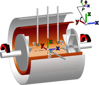
Figure 1: (Color online) Sketch of the VKS experiment

In the VKS experiment, a turbulent von Karman flow of liquid sodium is generated inside a cylinder by two counter-rotating impellers, with independent rotation frequencies $F_{1}$ and $F_{2}$ (see figure 1, and Berhanu09 for the description of the set-up). When $F_{1}=F_{2}$, the system is invariant about a rotation of an angle $\pi$ around any axis located in the mid-plane. On the contrary, if the impellers rotate at different rates, this symmetry, hereafter referred to as the $R_{\pi}$ symmetry, is broken. The dynamics of the magnetic field observed in the experiment strongly depend on this symmetry. When $F_{1}=F_{2}$, a statistically stationary magnetic field with either polarity is generated, with a dominant axial dipolar component. Dynamical regimes, including periodic oscillations and chaotic reversals of the magnetic field, are observed only when the $R_{\pi}$ symmetry is broken ($F_{1}\neq F_{2}$).

Previous studies have suggested that the evolution of the magnetic field in the VKS experiment results from low dimensional dynamics, involving only a few modes in interaction Ravelet08 . This can be ascribed to the proximity of the bifurcation threshold and to the smallness of the magnetic Prandtl number in liquid metals ($Pm<10^{-5}$). Indeed, in the low-$Pm$ regime, the magnetic field is strongly damped compared to the velocity field. Hence, the dynamics are governed only by a small number of magnetic modes. Based on this observation, Pétrélis and Fauve Petrelis08 have proposed that close to the dynamo threshold, the magnetic field can be decomposed into two components:

$${\bf B}=D(t)\,{\bf d}({\bf r})+Q(t)\,{\bf q}({\bf r})$$ (1)

where $D$ (respectively $Q$) represents the amplitude of dipolar ${\bf d}({\bf r})$ (resp. quadrupolar ${\bf q}({\bf r}$)) component of the field. As emphasized in Petrelis08 , these components do not only involve a dipole or a quadrupole, but also all the higher components with the same symmetry in the transformation $R_{\pi}$. In other words, ${\bf d}({\bf r})$ (resp. ${\bf q}({\bf r})$) is the antisymmetric (resp. symmetric) part of the magnetic field.

The evolution equations for $D(t)$ and $Q(t)$ can then be obtained by symmetry arguments (see Petrelis08 for a detailed description of the model). Since ${\bf d}\rightarrow-{\bf d}$ and ${\bf q}\rightarrow{\bf q}$ in the transformation $R_{\pi}$, dipolar and quadrupolar modes cannot be linearly coupled when $F_{1}=F_{2}$. Breaking the $R_{\pi}$ symmetry by rotating the impellers at different speeds allows a linear coupling between dipolar and quadrupolar modes. For a sufficiently strong symmetry-breaking, this coupling can generate a limit cycle that involves an energy transfer between dipolar and quadrupolar modes. This mechanism has been recently validated on a numerical model of the VKS experiment Gissinger09 and also in the case of a mean-field $\alpha^{2}$ dynamo model Gallet09 .

Two scenarios of transition from a stationary dynamo to a periodically reversing magnetic field can be described in the framework of this dipole-quadrupole model. When the coupling is such that the system is close to both a stationary and a Hopf bifurcation, i.e. in the vicinity of a codimension-two bifurcation point, one can have bistability between a stationary and a time periodic reversing dynamo Berhanu09 . We thus get a subcritical transition from a stationary dynamo to a periodic one with a finite frequency at onset. Turbulent fluctuations can generate random transitions between these two regimes Berhanu10 . Far from this codimension-two point, a reversing magnetic field can be generated through an Andronov bifurcation when the stationary state disappears through a saddle-node bifurcation Petrelis08 . Then, the frequency of the limit cycle vanishes at onset. In the vicinity of this transition, turbulent fluctuations drive random reversals of the magnetic field. As a consequence, random reversals always occur at the borderline between stationary and oscillatory dynamos. This simple mechanism also yields several predictions about the shape of the reversals. First, when the dipole $D$ vanishes, part of the magnetic energy is transferred to the quadrupole $Q$. An overshoot of the dipolar amplitude is expected after each reversal. Random reversals are asymmetric. During a first phase, fluctuations push the system from the stable solution to the unstable one, thus acting against the deterministic dynamics. This phase is slow compared to the one beyond the unstable fixed point, where the system is driven to the opposite polarity under the action of the deterministic dynamics.

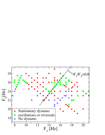
Figure 2: (Color online) Parameter space: (cross) no dynamo, (circle) stationary dynamos, (star) oscillatory or random reversing dynamos.

In this paper, we use data of the VKS experiment in order to reconstruct the dipolar and the quadrupolar parts of the magnetic field and study their behavior in the time dependent regimes. Time-dependent regimes only occur for specific values of $F_{1}$ and $F_{2}$, inside three delimited regions of the parameter space Berhanu10 . We will focus on the regimes observed when following the line $F_{1}/F_{2}=0.6$ in the parameter space. Figure 2 shows that when the rotation rates are increased along this line, one first bifurcates to a stationary dynamo, then to time-dependent regimes. Figure 3(top) shows the time-recordings of the three components of the magnetic field close to the fastest disk, displaying the bifurcation from stationary to time-dependent dynamo when the frequencies of the two disks are increased from $14.4/24$ Hz ($F_{1}+F_{2}=38.4$ Hz) to $15/25$ Hz ($F_{1}+F_{2}=40$ Hz). After a short transient state, the three components of the magnetic field undergo a transition to nearly periodic oscillations.

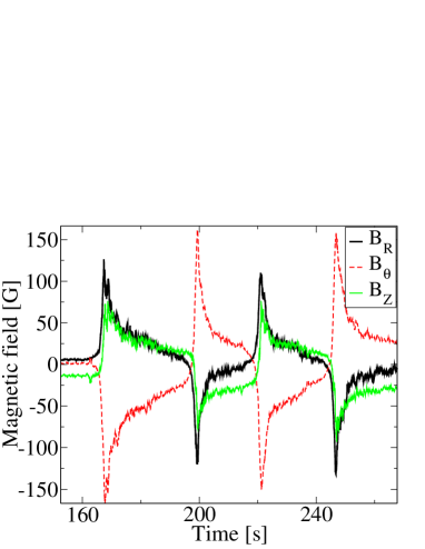
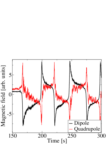
Figure 3: (Color online) Top: time recordings of the three components of the magnetic field. The rotation frequencies are increased from $14.4/24$ Hz to $15/25$ Hz, leading to a transition from a stationary low amplitude dynamo regime to a limit cycle. Bottom: Behavior of the dipolar and quadrupolar parts of the magnetic field. Note the transfer between the two components during reversals.

However, it is hard to test the pertinence of the model Petrelis08 from the time recording of the magnetic field at a single point. Using measurements obtained from two probes $1$ and $2$, symmetric with respect to the mid-plane, we compute the dipolar part, $D(t)d_{i}=(B_{i}(1,t)+B_{i}(2,t))/2$ and the quadrupolar part, $Q(t)q_{i}=(B_{i}(1,t)-B_{i}(2,t))/2$. In order to obtain observables which are independent of the spatial component $i$, each of these vectors is projected on its value at a given time $t_{0}$. We thus extract $D(t)$ and $Q(t)$ up to a multiplicative constant. In the measurements displayed here, the dipolar and quadrupolar components are projected on their stationary values obtained at $F_{1}+F_{2}=38.4$ Hz. Note however that different methods could be used to reconstruct these amplitudes. In particular, plotting the sum and the difference of a given component does not change the qualitative behavior GissingerThesis . Figure 3(bottom) shows the evolution of $D(t)$ and $Q(t)$ during periodic oscillations of the magnetic field. We observe that when the dipole vanishes, the amplitude of the quadrupole reaches its maximum. This shows that the field reversals observed in the VKS experiment do not correspond to a vanishing magnetic field, but rather to a change of shape from a dominant dipolar field to a quadrupolar one. Immediately after each reversal, one can also note that during its recovery, the dipolar amplitude strongly overshoots its mean value. Therefore, in agreement with the model Petrelis08 , reversals in the VKS experiment involve a strong competition between dipolar and quadrupolar components of the magnetic field.

The decomposition between dipolar and quadrupolar components is not only relevant to study these oscillations but is also useful to follow the bifurcations observed along the line $F_{1}/F_{2}=0.6$ in figure 2. We now investigate the evolution of the dynamics in the phase space $(D,Q)$ displayed in figure 4 as $F_{1}+F_{2}$ is modified. The limit cycle described in figure 3 bifurcates from a low amplitude stationary dynamo when $F_{1}+F_{2}$ is increased from $38.4$ to $40$ Hz. This limit cycle is shown in green in figure 4a. When $F_{1}+F_{2}$ is decreased again to $38.4$ Hz, a smaller amplitude limit cycle is obtained (orange curve, circles) instead of a fixed point. We need to decrease the rotation frequencies further to recover the low amplitude stationary dynamo (black dot). Therefore, this transition is hysteretic and within some frequency range we have bistability involving stationary and time-periodic dynamos. This oscillation appears at finite amplitude and finite period Berhanu10 . The oscillation of figure 3 displays a slowing down in the vicinity of two symmetric fixed points, as expected for a system close to the saddle-node bifurcation of Andronov type. Note however that the onset of the cycle when $F_{1}+F_{2}$ is increased, does not correspond to such a saddle-node bifurcation, since these two stagnation points are distinct from the low amplitude stationary dynamo regime obtained at $F1+F2=38.4$. In fact, this transition from a low amplitude stationary magnetic field to an oscillatory regime at finite period, rather corresponds to the model taken close to its codimension-two bifurcation point Berhanu09 .

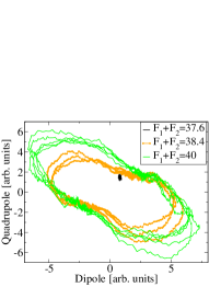
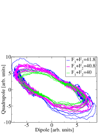
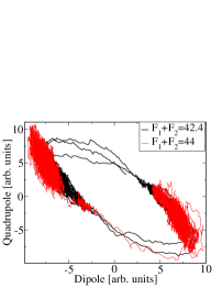
(a)

(b)

(c)

Figure 4: (Color online) (a): Evolution of the magnetic field in the phase space $(D,Q)$ at low frequencies: there exists a range of bistability in which a stationary dynamo (black dot) and a periodic limit cycle (orange circles) are both metastable. (b): Evolution of the limit cycle when $F_{1}+F_{2}$ is increased from $40$ to $41.8$ Hz. (c): Chaotic reversals obtained for large values of $F_{1}+F_{2}$ in the vicinity of a saddle-node bifurcation.

When $F_{1}+F_{2}$ is increased further, the amplitude of the limit cycle continuously increases (figure 4b). In addition, the system slows down in the vicinity of two points $(\pm D_{s},\pm Q_{s})$ (figure 4c). Thus, the period of the limit cycle significantly increases. For $F_{1}+F_{2}=44$ Hz, the systems stops on one of these two fixed points and we get a stationary dynamo (although we cannot rule out the occurrence of other reversals with a longer experiment). As explained in the framework of the model Petrelis08 , this second transition corresponds to a saddle-node bifurcation or more precisely an Andronov bifurcation: the stable fixed points $(\pm D_{s},\pm Q_{s})$ collide with unstable fixed points $(\pm D_{u},\pm Q_{u})$ when $F_{1}+F_{2}$ is decreased and disappear. A limit cycle is thus created, and its period is expected to diverge in the vicinity of the saddle-node bifurcation. Turbulent fluctuations of course saturate this divergence by kicking the system away from the points $(\pm D_{s},\pm Q_{s})$ where it slows down. They also strongly modify the dynamics on the other side of the bifurcation. Indeed, when the stable and unstable fixed points are very close one to the other, turbulent fluctuations can randomly drive the system from a stable fixed point to its neighboring unstable one, and thus trigger a reversal of the magnetic field. Therefore, random reversals are expected in the vicinity of the saddle-node bifurcation Petrelis08 . This is what is observed here as shown below.

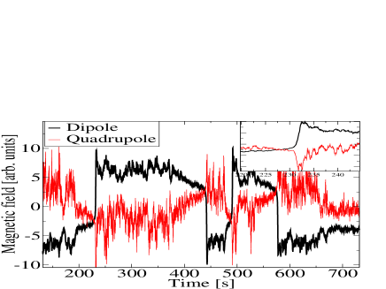
Figure 5: (Color online) Time evolution of the magnetic field during a regime of chaotic reversals, for $F_{1}+F_{2}=42.4$ Hz. Inset: zoom on the reversal occuring at $t=231$s.

Figure 5 displays the time-recordings of the dipolar and quadrupolar components for $F_{1}+F_{2}=42.4$ Hz. We observe that both components fluctuate around constant values as if they have reached a stable fixed point. The time spent in both polarities is random but much longer than the magnetic diffusion time scale (of order $1$ s). One also clearly observes that the amplitude of the dipole slowly decreases before rapidly changing sign. In the phase space $(D,Q)$ displayed in figure 4c, this slow decay corresponds to random motion in the regions in the form of elongated spots located along the limit cycle in the vicinity of the fixed points. Indeed, the motion from each stable fixed point to the neighboring unstable one, occurs under the influence of fluctuations acting against the deterministic dynamics. It is thus a slow random drift compared to the fast reversal phase driven by the deterministic dynamics once the system has been pushed beyond the unstable fixed point. Figure 4c also show that the spots become more and more elongated when $F_{1}+F_{2}$ is increased. This tells that the distance between each stable fixed point and its unstable neighbor increases. Correspondingly, reversals are less frequent. For $F_{1}+F_{2}=44$ Hz (red (light grey) cycle in figure 4c), fluctuations can hardly drive reversals. As for periodic oscillations obtained above the Andronov bifurcation, the modal decomposition $(D,Q)$ underlines the short transfer from an axial dipole to a quadrupolar magnetic field during random reversals obtained below the bifurcation threshold (see inset of figure 5). The dipolar amplitude displays the expected behavior, characterized by a slow decay followed by a rapid recovery, and showing a typical overshoot after each reversal. Evolution in the phase space $(D,Q)$ also illustrate how the transfer between dipolar and quadrupolar components yields very robust cycles, systematically avoiding the origin $B=0$.

In conclusion, we have used a simple method to extract the dipolar (antisymmetric) and quadrupolar (symmetric) components of the magnetic field in the VKS experiment. We have shown that this decomposition allows to investigate the morphology of the magnetic field during reversals, and to compare experimental results to the predictions of a recent model proposed in Petrelis08 . We have shown that the results of the VKS experiment are in very good agreement with these predictions:

- reversals are characterized by a strong transfer to the quadrupole when the dipole vanishes,

- the dipolar mode systematically displays an overshoot after each reversal,

- random reversals are asymmetric, i.e. involve two phases: a slow one triggered by turbulent fluctuations followed by a fast one mostly governed by the deterministic dynamics.

This agreement between the VKS experiment and the model has significant consequences. It first shows that a fluid dynamo, even generated by a strongly turbulent flow, can exhibit low dimensional dynamics, involving mostly dipolar and quadrupolar modes. Furthermore, because such a model is based on symmetry arguments, the mechanisms described here are expected to apply beyond the VKS experiment. For instance, although 3-dimensional simulations do not involve a similar level of turbulence, a transfer between dipole and quadrupole during reversals has been observed in several numerical studies of the geodynamo Glatz95 , CoeGlatz06 . This is consistent with indirect evidences from paleomagnetic measurements, suggesting a dipole-quadrupole interaction McFadden91 and asymmetric reversals Valet05 . Observations of the Sun’s magnetic field also suggest a transfer between dipolar and higher components Knaack05 . In numerical simulations based on the VKS experiment Gissinger10 , a good agreement with the three predictions reported here has been obtained, but only when the magnetic Prandtl number is sufficiently small. In this context, our simple method could be used to investigate data from numerical simulations of the geodynamo at low magnetic Prantl number. This opens new perspectives to understand the dynamics of planetary and stellar magnetic fields with a simple and low dimensional description.