On the generalization of wavelet diagonal preconditioning to the Helmholtz equation

Abstract

We present a preconditioning method for the multi-dimensional Helmholtz equation with smoothly varying coefficient. The method is based on a frame of functions, that approximately separates components associated with different singular values of the operator. For the small singular values, corresponding to propagating waves, the frame functions are constructed using ray-theory. A series of 2-D numerical experiments demonstrates that the number of iterations required for convergence is small and independent of the frequency. In this sense the method is optimal.

1 Introduction

In this paper we will describe a preconditioning method for a class of Helmholtz operators

$$H=-\Delta-\frac{\omega^{2}}{c(x)^{2}}+i\frac{\alpha(x)\omega}{Lc(x)},$$ (1)

where $c(x)$ and $\alpha(x)$ are positive, smoothly varying coefficents, $\omega$ is the frequency parameter, and $L$ is a typical length of the domain, which is inserted to make $\alpha$ dimensionless. See [3, 11, 14, 23, 27, 12, 13] for examples of preconditioners from the literature.

For elliptic equations there are good preconditioning methods, such as multigrid and wavelet diagonal preconditioning [6, 8]. Their effect can be explained using analysis in the position-wave number domain, the so called phase space. With this point of view we first give a short discussion of wavelet diagional preconditioning, and then turn to its generalization to the Helmholtz equation.

Consider, as an example problem an elliptic partial differential equation $Bu=f$, where $B$ is an invertible, symmetric, second order elliptic operator on a perioc domain (we will not go into the issues related to boundary conditions.) The main ingredients of the method are a basis transformation $F$, given by a wavelet transform, and an invertible diagonal scaling matrix $W$. The matrix $F^{*}$ is a wavelet reconstruction operator, its columns are the elements of the wavelet basis, denoted by $\psi_{\mu}$, $F$ is a wavelet decomposition operator. The elements of the diagonal of $W$ satisfy $w_{\mu}\sim 2^{-2|\mu|}$, where $|\mu|$ denotes the scale index of the wavelet, and by convention $|\mu|=-1$ corresponds to the scaling functions. A symmetrically preconditioned operator $B$ is then example given by an expression of the form

$$W^{1/2}FBF^{*}W^{1/2}.$$ (2)

Left- and right preconditioned variants also exist, they are given by $WFB$ and $BF^{*}W$.

The triple $(F^{*},W^{-1},F^{*})$ can be viewed as an approximate SVD. A true SVD $(U,S,V)$ would yield a perfect preconditioner, given by $S^{-1/2}U^{\prime}BVS^{-1/2}=I$. Equation (2) yields an approximation to the identity in the sense that $W^{1/2}FBF^{*}W^{1/2}$ is boundedly invertible, uniformly in parameters such as the grid constant.

The singular values of partial differential operators (PDO’s) with constant coefficients follow from Fourier analysis. The symbol of the operator is defined by

$$B(\xi)=e^{-ix\cdot\xi}(Be^{ix\cdot\xi}).$$ (3)

The singular functions are complex plane waves and the singular values $B(\xi_{\mu})$, with $\xi_{\mu}$ the wave vector. Wavelets are localized in the Fourier domain around $\|\xi\|=\pi 2^{|\mu|}$, away from zero and infinity, according to the vanishing moments and smoothness properties. Here being localized means that its Fourier transform decays rapidly away from some bounded region. Using this it can be shown that they act indeed as approximate singular function with value $\sim\pi^{2}2^{2|\mu|}$ [6, 9].

For variable coefficient PDO’s, or pseudodifferential operators, the analysis becomes more complicated, but in many cases similar results hold. The symbol becomes a function of $(x,\xi)$ [1, 21, 31]. If the symbol doesn’t vary too much over the area in phase space where a function is large, then one can often still show that the operator acts as an approximate multiplication by the value of its symbol at the phase space support, or is an approximate singular function. This idea is well known in semiclassical analysis, see e.g. [28, 25, 17, 18], and also occurs in numerical analysis [32].

With a wavelet basis is associated a tiling of phase space. The phase space can be divided into disjoint sets $\mathcal{T}_{\mu}$ that approximately correspond to the support of the wavelets. In 1-D, the multi-index $\mu$ has two components, $(j,k)$, and the tile is given by $2^{-j}[k,k+1]\times 2^{j}([\pi,2\pi]\cup[-2\pi,\pi])$ for $j\geq 0$ and by $[k,k+1]\times[-\pi,\pi]$ for $j=-1$. The tiling and the matrix $W$ are adapted to the operator $B$ in the following sense

$$C^{-1}\leq w_{\mu}\sigma_{B}(x,\xi)\leq C,\qquad\text{for all $(x,\xi)\in\mathcal{T}_{\mu}$, for all $\mu$.}$$ (4)

In words: The factor $w_{\mu}$ compensates for the action of the operator, which is an approximate multiplication, assuming the symbol doesn’t vary too much over the tile. This explains the choice of the wavelets and the matrix $W$, even if it cannot be taken literally and must be supplemented with appropriate technical arguments. The property (4) will serve as the guiding criterion for the design of a preconditioner for the Helmholtz operator.

Applying the criterion (4) to (1), one finds that the requirement that $F$ is a basis transform is very restrictive. To alleviate this requirement, methods based on frames have been proposed [30, 2, 20, 19]. If $F$ is a tight frame with $F^{*}F=I$, one can use a symmetric preconditioning of the form

$$F^{*}W^{1/2}FBF^{*}W^{1/2}F$$ (5)

Left- and right-preconditioned variants are given by

$$BF^{*}WF,\qquad\text{ and }\qquad F^{*}WFB.$$ (6)

A second form of left-preconditioning is given by $WFB$. The latter form leads to an overdetermined system of equations that is to be solved in the least-squares sense. The operators (5) and (6) are invertible if the diagonal entries of $W$ are real and strictly positive.

The criterion (4) has important consequences for the preconditioning of the Helmholtz equation. Let’s start with the situation that the coefficients $c$ and $\alpha$ are constant. Clearly a wavelet tiling can’t be used in a neighborhood of the set $\|\xi\|\approx\frac{\omega}{c}$. The wavelet will be of size $O(\omega)$ in the radial direction, and cover a wide range of values of the symbol from $|H(\xi)|=O(\omega)$ to $|H(\xi)|=O(\omega^{2})$. Based on the criterion they can only be used some distance $O(\omega)$ away from this set. Therefore, the generalization of wavelet diagonal preconditioning to the Helmholtz equation must use a different set of basis or frame functions, with a different phase space tiling.

The tiling must be such that the tiles around $\|\xi\|=\frac{\omega}{c}$ must be of size at most $O(1)$ in the radial Fourier direction. It follows that they are of size $O(1)$ in the corresponding spatial direction. In other words, the frame functions have a macroscopic spatial extent, also when $\omega$ increases and the wavelength becomes smaller. This conclusion can also be reached from a completely different way, by considering the flow of information in an iterative algorithm. The distance the information can travel is proportional to the size of the support of the frame functions. Since we aim at convergence in a number of steps independent of $\omega$, and since the solutions of $Hu=f$ contain waves propagating over $O(1)$ distance, there must be frame functions with $O(1)$ size of the support, and it is natural that these correspond to the propagating wavenumbers with $\|\xi\|\approx\frac{\omega}{c}$. One can also observe that the number of frame functions with small approximate singular values is much larger than for the elliptic case, it is on the order of $O(1)$ time the area of the set $\|\xi\|=\frac{\omega}{c}$. If the number of points per wavelength is kept constant while $\omega$ may vary, this leads to $O(N^{d-1})$ basisfunctions with small eigenvalues, where $N$ is the number of grid points in each direction, and $d$ is the dimension. For constant coefficients of course a Fourier basis can be used.

In case of variable coefficients the situation becomes more complicated. The tiles with small value of the symbol $|H(x,\xi)|$ must satisfy $\|\xi\|\approx\frac{\omega}{c(x)}$ over an $O(1)$ domain. The wavenumber content of the basisfunction must depend on the position. The frame functions must therefore be adaptively chosen, depending on $c$ and $\omega$. This is unlike many existing phase space transforms [24], and also unlike certain transforms that have been used for hyperbolic PDE (but not for preconditioning) [7, 29, 5].

In this paper we show that it is possible to construct such a frame. The construction uses the WKB approximation in combination with a paraxial approximation for the wave equation (because ray theory is used it can be compared with the work of Brandt and Livshits [3, 23] except that they treated the variable coefficient case only in one dimension.) Our second main result concerns the convergence of the preconditioned operator. Using an implementation in Matlab we find that the number of steps required to converge becomes bounded by a small number, independent of the frequency.

While the number of steps is small, the cost per step is still relatively high. Further research into these transforms might improve this, as could the fast algorithm of [4] for the 3-D case. We find that larger problems can be solved than with the direct method because the memory requirement is reduced. The computation is split in two steps, a preparation step and an execution step, such that the results of the preparation step can be reused for each right hand side. We find that the computation time for the execution step is lightly increased compared to the direct method. The smoothness requirement on the medium, the inclusion of other boundary conditions or a damping layer, and the extension to the 3-D case are topics for further research.

The remainder of the paper is structured as follows. In section 2 some properties of our class of Helmholtz operators are discussed. The construction of the preconditioner in the continuous setting is the topic of sections 3 and 4. Some aspects of the discretization and implementation are then explained in section 5. Section 6 shows the results of our numerical experiments. We end with a short discussion.

2 A class of Helmholtz operators

The class of Helmholtz operator we study is given in (1). We assume that there are constants $C_{1}$ and $C_{2}$ such that

$$0<C_{1}\leq c(x)\leq C_{2}.$$ (7)

The imaginary part of $H$ is responsible for damping. We assume $\alpha(x)$ is $O(1)$ throughout the domain. So there must be $C>0$ such that

$$\frac{1}{C}\leq\alpha(x)\leq C.$$ (8)

We assume the domain is rectangular. For simplicity, the boundary conditions are assumed to be periodic. The spatially varying wave length is given by $\frac{2\pi c(x)}{\omega}$. The situation of interest is when the domain is many wave lengths large, but not so large that a discretization of the Helmholtz equation becomes impossible.

With the periodic boundary conditions the part of $H$ without the imaginary coefficient, which we denote by

$$H_{1}=-\Delta-\frac{\omega^{2}}{c(x)^{2}}$$ (9)

is real and selfadjoint. It has real eigenvalues that may be close to zero. The imaginary part influences the singular values of the operators $H$ and $A$. It leads to the lower bound

$$\|Hu\|\geq\frac{\alpha_{\rm min}\omega}{Lc_{\rm max}},$$ (10)

where $\alpha_{\rm min}$ is the minimum of $\alpha$ over the domain, and $c_{\rm max}$ the maximum of $c$.

We consider a finite difference approximation $A$ of $H$ based on the standard five point stencil for the Laplacian

$$(Au)_{i,j}=\frac{1}{h^{2}}\left(4u_{i,j}-u_{i+1,j}-u_{i-1,j}-u_{i,j+1}-u_{i,j-1}\right)+\left(-\frac{\omega^{2}}{c_{i,j}^{2}}+\frac{i\alpha_{i,j}\omega}{Lc_{i,j}}\right)u_{i,j}.$$ (11)

The preconditioning method is based on the properties of the continuous operator, therefore we expect the results to be valid for other discretizations as well, as long as they approximate the continuous problem with reasonable accuracy, see also the remarks later on. Setting $\alpha_{i,j}$ to zero in (11) yields the finite difference approximation $A_{1}$ of $H_{1}$. The matrix $A_{1}$ is real and selfadjoint, like $H_{1}$, so that $A$ satisfies

$$\|Au\|\geq\frac{\alpha_{\rm min}\omega}{Lc_{\rm max}}.$$ (12)

Based on the largest eigenvalue of the discrete Laplacian, given by $8h^{-2}$, we find the following estimate for $A$

$$\|Au\|\leq\left|\frac{8}{h^{2}}-\frac{\omega^{2}}{c_{\rm max}^{2}}+i\frac{\omega}{\alpha_{\rm max}Lc_{\rm min}}\right|\,\|u\|.$$ (13)

The number of points in the domain, and the grid size $h$ are in practice often chosen based on the number of wavelengths that fit in the domain. For example using a rule to keep a certain number of points, say $N_{\rm w}$, per wavelength. Reasonable values are of the order of 15 or 20. This means

$$h=\frac{2\pi c_{\rm min}}{N_{\rm w}\omega}.$$ (14)

Equations (12) and (13), and the assumption that $\alpha$ is not too large, so that
$\left|\frac{8}{h^{2}}-\frac{\omega^{2}}{c_{\rm max}^{2}}+i\frac{\omega}{\alpha_{\rm max}Lc_{\rm min}}\right|\leq\frac{8}{h^{2}}$ imply the following bound for the condition number

$$\mathcal{K}(A)<\frac{2LN_{\rm w}^{2}\omega c_{\rm max}}{\pi^{2}\alpha_{\rm min}c_{\rm min}^{2}}.$$ (15)

In other words $\mathcal{K}(A)\sim\omega$ if $\omega\rightarrow\infty$ with the given choice of $h$.

We have made the particular choice that the damping term has coefficient $O(\omega)$. This leads to the suppression of certain resonance effects, where small eigenvalues occurring around specific frequencies lead to numerical difficulties. At the same time, the solution to Helmholtz equation still consist of propagating waves with propagation distance on the order of the domain length. A damping term $O(\omega^{2})$ would lead to a propagation distance on the order of a fixed number of wavelengths when $\omega\rightarrow\infty$. The problem would become essentially elliptic. For elliptic equations, wavelet or multigrid preconditioning methods lead to a uniformly bounded operator, i.e. the problem of finding a preconditioner is essentially solved. The resonance effect that were just mentioned depend on subtle global properties of the medium. Some of the small singular values can likely be removed by using outgoing radiation boundary conditions, but it appears that internal wave patterns can also lead to large values for the norm of the resolvent. In this respect it could be interesting to study consequences of the results from the semiclassical analysis of the Schrödinger operator and its resonances, see e.g. [16]. It is clear that the ideas of this paper do not take into account the global properties referred to, so we make no claims concerning the situations without damping present.

3 Frame transform adapted to the Helmholtz operator in one dimension

In this section we design a frame transform adapted to the Helmholtz operator with the domain $[0,1]$ and periodic boundary conditions. The frame transform will consist of two steps. First we separate the function into three components that are essentially supported in three regions of phase space: The large wave numbers, the positive wave numbers of wavelength scale, and the negative wave numbers of wave length scale. The small wave numbers (smaller than wavelength scale) are treated together with the wavelength scale wave numbers. For each of these components a transform corresponding to a tiling is applied: Fourier tiling for the large wave numbers, and a modulated Fourier tiling (associated with a modulated Fourier transform) for the wave length scale wave numbers. The modulation parameter is a spatial function depening on the function $c$, and will cause the required curved space tiling. The idea of a modulated Fourier transform for preconditioning is new to our knowledge.

We first apply a windowing operator

$$G:u\mapsto\begin{pmatrix}u_{1}\\ u_{2}\\ u_{3}\end{pmatrix}$$ (16)

using

$$\hat{u}_{1}(\xi)=\chi_{1}(\xi)\hat{u}(\xi),\qquad\hat{u}_{2}(\xi)=\chi_{2}(\xi)\hat{u}(\xi),\qquad\hat{u}_{3}(\xi)=\chi_{3}(\xi)\hat{u}(\xi)$$ (17)

The function $\chi_{j}\in C^{\infty}(\mathbb{R})$ to minimize to keep signals localized in space. They must satisfy $\sum_{j=1}^{3}\chi_{j}^{2}=1$, then this map satisfies $G^{*}G=I$, so that a tight frame can be constructed. The function $\chi_{1}$ will be supported away from the zero set of the real part of the symbol, we require $\chi_{1}(\xi)=0$ on $[-1.5\omega/c_{\rm min},1.5\omega/c_{\rm min}]$. The function $\chi_{2}$ will be supported around the positive zero set of $H_{1}$. We require $\chi_{2}(\xi)=0$ outside $[-0.4\omega/c_{\rm max},2\omega/c_{\rm min}]$. Similarly, the function $\chi_{3}$ will be supported around the negative zero set of $H_{1}$, and $\chi_{3}(\xi)=0$ outside $[-2\omega/c_{\rm min},0.4\omega/c_{\rm max}]$. Within the overlap regions $[-2\omega/c_{\rm min},-1.5\omega/c_{\rm min}]$, $[-0.4\omega/c_{\rm max},0.4\omega/c_{\rm max}]$, $[1.5\omega/c_{\rm min},2\omega/c_{\rm min}]$ we use a dilated and translated version of a smooth cutoff function $h(x)$, such that $h(1-x)^{2}+h(x)^{2}=1$, and given by [2]

$$h(x)=\left\{\begin{array}[]{ll}0&\text{if}\quad x\leq 0,\\ \sin\left(\frac{\pi}{2}\frac{e^{-\frac{c}{x}}}{e^{-\frac{c}{x}}+e^{-\frac{c}{1-x}}}\right)&\text{if}\quad 0<x<1,\\ 1&\text{if}\quad x\geq 1.\end{array}\right.$$ (18)

For each of the $u_{j}$ we use a basis transform. For $u_{1}$ we use the standard Fourier transform

$$v_{j}=e^{ix\xi_{j}}$$ (19)

The operator $-\partial_{x}^{2}-\omega^{2}/c(x)^{2}$ acts on this as

$$P_{1}v_{j}=(\xi_{j}^{2}-\omega^{2}/c(x)^{2})v_{j}$$ (20)

The preconditioning factor is

$$\left((\xi_{j}^{2}-\omega^{2}/c_{\rm mean}^{2})^{2}+\left(\frac{\omega}{c_{\rm mean}}\right)^{2}\right)^{-1/2}$$ (21)

For $u_{2}$ we use the functions

$$v_{j}=e^{i\omega T(x)+ix\xi_{j}}$$ (22)

with $T(x)=\int_{0}^{x}c(s)^{-1}\,ds$ (the travel time), or with a small linear term added, so that $\omega(T(1)-T(0))/(2\pi)\in\mathbb{Z}$ and $e^{i\omega T}$ hence satisfies the periodic boundary conditions. The values of $\xi_{j}$ are $\xi_{j}=2\pi j$. The addition of the term $i\omega T(x)$ causes an additive shift in the so called instantaneous phase [24] by $\omega\frac{\partial T}{\partial x}$. The rectangular tiles associated with the Fourier modes $v_{j}e^{ix\xi_{j}}$ hence receive an $x$-dependent shift in the vertical direction of the $(x,\xi)$ plane. The tiling associated with this basis is given by

$$0\leq x\leq 1,\qquad\frac{\omega}{c(x)}+\xi_{j}-\pi<\xi<\frac{\omega}{c(x)}+\xi_{j}+\pi,\qquad j\in\mathbb{Z}.$$ (23)

We define the scaling factor for preconditioning by

$$w_{j}=\left(\left(\frac{\omega}{c(x)}\right)^{2}+\left(2\frac{\omega}{c(x)}\xi_{j}\right)^{2}\right)^{-1/2}.$$ (24)

because we find that the value of the symbol can be uniformly estimated by $w^{-1}$ on the intersection of the support of $u_{2}$ and the domain of the tile. The tiling for an example $c(x)$ is displayed in Figure 1. We treat $u_{3}$ similarly with

$$v_{j}=e^{-i\omega T(x)+ix\xi_{j}},$$ (25)

and preconditioning factor given again by (24). Denoting by $F$ the full transform, it follows that $F^{*}F=I$, i.e. the transform corresponds to a tight frame.

Instead of (22) and (25) it is also possible to use modulated wavelets, see the tiling in Figure 1. This can be attractive because a wavelet transform has cost $O(N)$, versus $O(N\log N)$ for the Fourier transform.

Some computations using the above methods that were done early on in this research gave encouraging results. As the focus of this paper is on the multi-dimensional case we will not further report on this here.

(a)

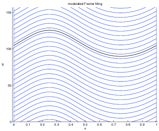
(b)

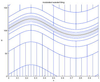
Figure 1: Example of curved phase space tilings adapted to $H$ for $\xi\geq 0$. (a) Modulated Fourier tiling; (b) modulated wavelet tiling.

4 Frame transform adapted to the higher-dimensional Helmholtz operator

In this section we devise a frame of functions, assocatiated with a tiling of phase space adapted to $|H(x,\xi)|$, in dimension $d=2$ or higher. The construction is done in the continuous setting. Discretization and implementation aspects are discussed in the next section.

Like in the one-dimensional case the most challenging region of phase space is around the zero-set (characteristic set) of the real part $H_{1}$, given by

$$\operatorname{Char}(H_{1})=\left\{(x,\xi)\in\mathbb{T}^{d}\times\mathbb{R}^{d}\,;\,\|\xi\|=\frac{\omega}{c(x)}\right\}.$$ (26)

Here $\mathbb{T}^{d}$ denotes the $d$-dimensional torus, also written as $[0,1]^{d}$ with periodic boundary conditions. In the Fourier space, the direction normal to $\operatorname{Char}(H_{1})$, a tile has size at most $O(1)$, implying that the size in the corresponding spatial direction is at least $O(1)$. The tile must follow the curved surface of $\operatorname{Char}(H_{1})$, a property not present in existing multi-dimensional transforms, see e.g. Mallat [24].

Just like the previous section we will not construct a single, global tiling. Instead the first step of the frame transform is a division into different regions of phase space. Regions associated with sufficiently large and sufficiently small wave numbers can be treated with Fourier preconditioning. The other regions are chosen such that the part of characteristic set they contain is a graph, say $\xi_{j}=f(x,\xi_{1},\ldots,\xi_{j-1},\xi_{j+1},\ldots,\xi_{n})$. We call $x_{j}$ the preferred coordinate. We summarize the remainder of the construction. Locally in phase space the Helmholtz equation becomes equivalent to a first order evolution equation in the preferential direction. Using theory for hyperbolic pseudodifferential equations an abstract frame is constructed. To obtain a computable set of functions a WKB approximation is made, which finally yields the result.

So the first step in the frame transform is the separation of $u$ into components that live in different regions of phase space. Localization is done in the Fourier space in radius (scale) and angle, and in the position space to certain rotated rectangular regions. There are three wave numbers scales, the small wave numbers $\|\xi\|<\omega/c_{\rm max}$, the wave length scale wave numbers $\omega/c_{\rm max}\leq\|\xi\|\leq\omega/c_{\rm min}$, and the large wave numbers $\|\xi\|>\omega/c_{\rm min}$. We will use a map $F_{\rm scale}:u\mapsto\begin{pmatrix}u_{1}\\ u_{2}\\ u_{3}\end{pmatrix}$ using

$$\hat{u}_{1}(\xi)=\chi_{1}(\xi)\hat{u}(\xi),\qquad\hat{u}_{2}(\xi)=\chi_{2}(\xi)\hat{u}(\xi),\qquad\hat{u}_{3}(\xi)=\chi_{3}(\xi)\hat{u}(\xi)$$ (27)

with three smooth cutoff functions $\chi_{j}(\xi)$, $j=1,2,3$ to separate the small, wavelength scale and large wave numbers. Again the cutoff functions will satisfy $\sum\chi_{j}^{2}=1$ to have $F_{\rm scale}^{*}F_{\rm scale}=I$. By $k_{1},k_{2}$ we denote constants to separate the low and wave length scale wave numbers. For $\|\xi\|$ going from $k_{1}$ to $k_{2}$ $\chi_{1}$ goes smoothly from one to zero and $\chi_{2}$ smoothly from 0 to 1 according to the standard cutoff function $h$. By $k_{3},k_{4}$ we denote constants to separate the wavelength scale and high wavenumbers.

For further localization in the Fourier space, we will distinguish several directions in the Fourier space, each direction described by a unit vector $\alpha\in S^{d-1}$. Using cutoffs, the support in the Fourier domain will be restricted to angular wedges around each angle $\alpha$. This angle will also determine the spatial localization. We consider new coordinates $(y,z)$, with $y$ in $\alpha$ direction and $z=(z_{1},\ldots,z_{d-1})$ normal to this direction. We cover the spatial domain with a small number of coordinate boxes in these coordinates. The new coordinates will have $y=0$ in the center of each box. Because of the periodic boundary conditions, in our 2-D numerical examples we chose periodic bands. To obtain this, $\alpha$ is set such that $\tan(\alpha)$ is a ratio of two small integers.

After phase space localization and coordinate transform, the preconditioning can be done according to the following symbol, for which we locally have $P\sim H_{1}$

$$P=2\frac{\omega}{c_{\rm mean}}\left(\eta-\sqrt{\frac{\omega^{2}}{c(y,z)^{2}}-\zeta^{2}}\right).$$ (28)

Moreover, this can be further modified outside the region of phase space that the analysis was restricted to. Here this is useful to deal with the singularity of the square root at $\|\zeta\|=\frac{\omega}{c(y,z)}$. We define a $C^{2}$ function by

$$S(s_{z})=\left\{\begin{array}[]{ll}\sqrt{1-s_{z}^{2}}&\text{if $|s_{z}|\leq\sin(\alpha)$}\\ \cos(\alpha)-(|s_{z}|-\sin(\alpha))\tan(\alpha)&\text{if $|s_{z}|>\sin(\alpha)$},\end{array}\right.$$ (29)

and instead of (28) the following symbol $P\sim H_{1}$ will be used

$$P=2\frac{\omega}{c_{\rm mean}}\left(\eta-\frac{\omega}{c(y,z)}S(\frac{\zeta c(y,z)}{\omega})\right).$$ (30)

The function

$$B(y,z,\zeta,\omega)=\frac{\omega}{c(y,z)}S(\frac{\zeta c(y,z)}{\omega})$$ (31)

is a symbol (here we ignore that $S$ is only $C^{2}$ instead of $C^{\infty}$, because a smoother symbol can be designed if the numerical computations require it). We define an operator $B(y,z,D_{z})$ by

$$B(y,z,D_{z})u(y,z)=(2\pi)^{-(d-1)}\iint(B(y,z,\zeta)+\text{l.o.t.})e^{iz\cdot\zeta}\hat{u}(y,\zeta)\,d\zeta.$$ (32)

For later reference we also define a pseudodifferential operator $B(y,z,D_{z},D_{t})$ that acts on function of $(z,t)$, with $t$ a time coordinate

$$B(y,z,D_{z},D_{t})u(y,z,t)=(2\pi)^{-d}\iint(B(y,z,\zeta,\omega)+\text{l.o.t.})e^{iz\cdot\zeta-i\omega t}\hat{u}(y,\zeta,-\omega)\,d\zeta\,d\omega.$$ (33)

In these equations $\hat{u}$ defines a Fourier transform w.r.t. a subset of the variables as indicated. We will assume the lower order terms are such that $B(y,z,D_{z})$ and $B(y,z,D_{z},D_{t})$ are real and selfadjoint, see e.g. [26]. The differential equation assocated with (30) is

$$\left(\partial_{y}-iB(y,z,D_{z})\right)u(y,z)=0.$$ (34)

It is an evolution equation in $y$.

Equation (34) is of a well known type, it is called a one-way wave equation. The unknown $u$ can be considered as a function of $(y,z,\omega)$. After Fourier transform $-\omega\mapsto t$, this results in a first order hyperbolic pseudodifferential equation results, see e.g. [21, 31] for the theory of such equations. One-way wave equations are a tool for the analysis of hyperbolic systems of equations, as well as for their numerical computation, see [26] and the references therein. Because of their nature, they eiter describe waves propagating in the positive $y$ direction, or in the negative $y$ direction. So called ’turning waves’, for which the $y$-component of the propagation direction changes sign, are not described by such an equation. Propagation under large angles with the $y$-axis is also a problem for numerical methods for one-way wave equations. These usually become inaccuarate if the angle is too large, e.g. larger than 60 degrees.

By $E(y,y_{0})$ we will denote a solution operator, meaning if $u_{0}=u_{0}(z)$ are initial conditions at $y_{0}$, then

$$(\partial_{y}-iB)E(y,y_{0})u=0,\qquad E(y_{0},y_{0})u=u.$$ (35)

We define the operator $T$, acting on a function of $(y,z)$, by

$$Tu(y,\cdot)=E(y,0)u(y,\cdot)$$ (36)

From the assumption that the operator $B=B(y,z,D_{z})$ is self-adjoint it follows that this operator is unitary, $T^{*}T=I$. We find that

$$\begin{split}(\partial_{y}-iB)E(y,0)u(y,\cdot)={}&\left((\partial_{y}-iB)E(y,0)\right)u(y,\cdot)+E(y,0)\partial_{y}u\\ ={}&E(y,0)\partial_{y}u,\end{split}$$ (37)

i.e. the following intertwining operator relation holds

$$(\partial_{y}-iB)T=T\partial_{y}.$$ (38)

Let $\hat{\phi}_{\mu}(y)$, $\tilde{\phi}_{\nu}(z)$ be frames, and suppose the frame $\hat{\phi}_{\mu}(y)$ is adapted to the operator $\partial_{y}+1$ in the sense discussed above, with preconditioning factors $w_{\mu}$. We define a candidate for our frame by

$$\phi_{\mu,\nu}(y,z)=T\hat{\phi}_{\mu}(y)\tilde{\phi}_{\nu}(z).$$ (39)

Since $T$ is unitary the new frame is also a tight frame with frame bound $1$. Indeed,

$$\begin{split}\sum_{\mu}|\langle\tilde{\phi_{\mu}},f\rangle|^{2}={}&\sum_{\mu}|\langle T\phi_{\mu},f\rangle|^{2}=\sum_{\mu}|\langle\phi_{\mu},T^{*}f\rangle|^{2}\\ ={}&\langle T^{*}f,T^{*}f\rangle=\|f\|^{2}.\end{split}$$ (40)

We use the intertwining property and the unitarity property, to argue that the preconditioning weights should be $w_{\mu}$. A matrix element satisfies

$$\langle\phi_{\kappa,\lambda},(\partial_{x}-iB)\phi_{\mu,\nu}\rangle=\langle\hat{\phi}_{\kappa}\tilde{\phi}_{\lambda},T^{*}(\partial_{y}-iB)T\hat{\phi}_{\mu}\tilde{\phi}_{\nu}\rangle=\langle\hat{\phi}_{\kappa},\partial_{y}\hat{\phi}_{\mu}\rangle\langle\tilde{\phi}_{\lambda},\tilde{\phi}_{\nu}\rangle,$$ (41)

hence, taking into account the factor $\frac{2\omega}{c_{\rm mean}}$ in (28), $\frac{c_{\rm mean}}{2\omega}w_{\mu}$ is a good choice for the preconditioning factors.

Actual application of the frame transform associated with (39) requires the computation of $E(y,0)\tilde{\phi}_{\nu}(z)$. This amounts to solving the initial value problem for a first order hyperbolic pseudodifferential equation. There are various methods to solve one-way wave equations numerically, see [26] and references. Here we will use a different, semi-analytical approach, and use the WKB approximation. It is assumed that the frame property of the $\phi_{\mu,\nu}$, and the property that it yields is a good preconditioner are stable against the (small) perturbations due to the errors in the WKB approximation.

For $E(y,0)\tilde{\phi}_{\nu}(z)$ we therefore look for solutions of the form

$$A(y,z)e^{i\phi(y,z)}.$$ (42)

The “initial values” $\tilde{\phi}_{\nu}$ must be of the form $A(z)e^{i\phi(z)}$. Making use of our periodic setting, we choose a Fourier basis for $\phi_{\nu}$ (here $\nu=k\in\mathbb{Z}$)

$$\tilde{\phi}_{k}=L_{2}^{-1/2}e^{ix(2\pi k/L)}.$$ (43)

An alternative would be a windowed Fourier frame $\tilde{\phi}_{k,m}=w(y-kv_{0})e^{im\zeta_{m}}$.

Let’s start with the equation for $\phi$. We write $\phi=\omega T(y,z)$, where $T$ has the dimension of time. The initial conditions for $T$ are $T(0,z)=\frac{2\pi k}{\omega L}z$. The WKB method gives the following equation for $T$

$$\frac{\partial T}{\partial y}=S(\frac{c}{\omega}\frac{\partial T}{\partial z}).$$ (44)

Without the regularization of (29) this becomes a well-known equation,

$$\frac{\partial T}{\partial y}-\sqrt{\frac{1}{c^{2}}-\left(\frac{\partial T}{\partial z}\right)^{2}}=0,$$ (45)

the eikonal equation as an evolution equation in the $y$ direction. Equation (44) can be solved e.g. by upwind finite differences.

The amplitudes for the equation satisfy a transport equation along the characteristics [15]. Let $Z(y,z)$ describe a set of characteristics. The fact that $E$ is unitary provides an additional relation, namely that

$$A(y,Z(y,z_{0}))=A(0,z_{0})\left(\frac{\partial Z}{\partial z_{0}}\right)^{-1/2}.$$ (46)

Instead of computing the characteristics, it is convenient to compute $Z_{0}(y,z)$, the inverse of the map $z_{0}\mapsto Z(y,z_{0})$. This function satisfies itself a transport equation that can be solved along with $T(y,z)$.

The last step in describing the frame functions is the choice of $\hat{\phi}_{\mu}(y)$. We choose again the Fourier modes, $\mu=j$, $\hat{\phi}_{j}(y)=e^{i2\pi j/(2L_{1})}$.

Having described the frame functions, we look at the resulting transform, which, we recall is defined by taking

$$\langle\phi_{\mu,\nu},f\rangle=\iint\overline{\phi_{\mu,\nu}(y,z)}f(y,z)\,dz\,dy.$$ (47)

This amounts to two steps. First the map

$$F_{1}u(y,\zeta_{k})=\int A(y,\zeta_{k},z)e^{i\omega T(y,\zeta_{k}/\omega,y)}u(y,z)\,dz.$$ (48)

This is a Fourier integral operator. Then the map

$$c_{j,k}=\mathcal{F}_{x\mapsto j}(F_{1}u(y,\zeta_{k})).$$ (49)

We will call the frame transform a Lagrangian wave packet transform because of the tiling, which, as discussed below, is associated with a canonical relation that is by definition a Lagrangian manifold.

We have already discussed that, if $u$ is considered as a function of $(y,z,\omega)$, and after inverse Fourier transform $-\omega\mapsto t$, in short, in the time domain, equation (34) becomes a first order hyperbolic pseudodifferential equation. In the time domain the operator $T$ is a Fourier integral operator. This is useful, because the theory of Fourier integral operators also includes a geometrical description of the mapping of energy in the phase space, which results (for large $\omega$) in the description of the mapping of singularities. The mapping of singularities is according to the canonical relation [10, 22, 33, 31]. The canonical relation for the solution operator to first order hyperbolic systems is described in terms of the bicharacteristics, i.e. the characteristics of the eikonal equation. We use the notation $B(y,z,\zeta)$ for the (principal) symbol of the pseudodifferential operator $B$. The bicharacteristics are described by the system of ODE’s

$$\frac{\partial z}{\partial y}={} -\frac{B}{\zeta}$$

$$\frac{\partial\zeta}{\partial y}={} \frac{B}{z}.$$

Based on the unregularized operator (28), the explicit equations are

$$\frac{\partial z}{\partial y}={} \zeta\left(\frac{\omega^{2}}{c^{2}}-\zeta^{2}\right)^{-1/2},$$

$$\frac{\partial\zeta}{\partial y}={} -\frac{\omega^{2}}{c^{3}}\frac{\partial c}{\partial z}\left(\frac{\omega^{2}}{c^{2}}-\zeta^{2}\right)^{-1/2}.$$

Denote by $(Z(y,z_{0},\zeta_{0}),\Theta(y,z_{0},\zeta_{0}))$ the solution operator that describes the flow with initial values $(z_{0},\zeta_{0})$ at $y=0$. Let $\hat{\mathcal{T}}_{\mu}$ be the tiling associated with $\hat{\phi}_{\mu}$, and $\tilde{\mathcal{T}}_{\nu}$ be the tiling associated with $\tilde{\phi}_{\nu}$. This results in the following description of the tiling

$$\mathcal{T}_{\mu,\nu}=\{(y,Z(y,z_{0},\zeta_{0});\eta+B(y,Z,\Theta),\Theta(y,z_{0},\zeta_{0}))\,;\,(z_{0},\zeta_{0})\in\tilde{\mathcal{T}}_{\nu},(y,\eta)\in\hat{\mathcal{T}}_{\mu}\}.$$ (50)

5 Implementation aspects

In this section we discuss some aspects of the implementation of the frame transform and the preconditioner outlined in the previous section. The two main steps to be performed for the frame transform are the localization in phase space in scale and in angle described in the first part of this section, and the transform described in (48) and (49). We will comment on the discretization of each of those steps, and then say a few words on the structure of a program implementing the preconditioner.

The localization in scale in the Fourier domain was described in the text around (27). This is straightforward to discretize. We choose $k_{1}=0.2\omega/c_{\rm max}$, $k_{2}=\omega/c_{\rm max}$, $k_{3}=1.0\omega/c_{\rm min}$, $k_{4}=1.4\omega/c_{\rm min}$. The algorithm appears to be insensitive to the detailed values. In connection with the subsampling step described below, it is advantageous to use smaller values of $k_{4}$ if possible. For the windowing in angle we use $N_{\rm a}=8$ angles, $-225,-180,\ldots,90$ degrees. Three subsequent angles are used to define a cutoff function in angle, using appropriately translated and dilated versions of the standard cutoff $h$.

After windowing in the Fourier domain a subsampling step is done. After localization, the Fourier transform of the signal is supported in a small subdomain of the original domain. A rectangle is taken that contains this subdomain, and the Fourier grid within the rectangle is used for the further calculations. This results in a function defined on a substantially coarser grid in space.

The final step associated with the restriction in the phase space is the rotation to the new spatial coordinates $(y,z)$, and a resorting of the data into periodic bands. The rotation amounts to interpolation to a rotated grid. This is done by shear rotation which is an exactly invertible operation. It changes the grid parameters, but that is not a problem. The shear rotation is combined with the resorting of the data in periodic bands. The details of the bands depends on the angle. The total number of bands will be denoted by $N_{\rm b}$. The bands are chosen overlapping, and a cutoff function in the $y$ coordinate is applied.

For the application of the Fourier integral operator, first a preparation step needs to be done computing $T(y,z,p_{z})$ and $A(y,z,p_{z})$. The travel time $T(y,z,p_{z})$ is computed using upwind finite differences. These are also used to compute $Z_{0}(y,z,p_{z})$. $A$ is then computed from (46). The storage for $A(y,\zeta_{k},z)e^{i\omega T(y,\zeta_{k}/\omega,y)}$ is the largest storage requirement for the algorithm. For an $d$ dimensional domain with discretization size $N$ in each direction, and subsampling toward $\beta N$ in each direction, this is about $2N_{\rm a}(\beta N)^{3}$. Some numbers from the numerical experiments are given in the next section.

Application of the Fourier integral operator in (48) is done simply by replacing the integral by a summation. We have experimented with a partial implementation of the scheme described in [4], but there were no significant gains, this was partially related to the large subsampling we did before computing (48).

This leads to the following program structure. First all preparatory tasks are performed by a routine prepare_helmprec. The main steps are two call the two routines prepare_filter_band and prepare_lwpt, that prepare the filtering and banding step, respectively the Lagrangian wave packet transform. The results are stored and make it possible to apply the preconditioner rapidly each time it is called. The actual execution of the preconditioner is done by a routine execute_helmprec. A similar subdivision is made, a routine execute_filter_band executes the transform from input data to the filtered and banded data, and the adjoint of this operation. A routine execute_lwpt computes the forward version or the adjoint of the transform described in (48) and (49). It is straightforward to apply the scaling factors $w_{\mu}$.

6 Numerical results

The purpose of our numerical experiments is to study the convergence of the method. The convergence depends on the problem parameters, the function $c$, the frequency $\omega$, the damping parameter and the right hand side of the equation. Of this, the dependence on $c$ and on $\omega$ are the most interesting, and we will show some results for different values of $c$ and $\omega$. We have fixed the damping to $\alpha=2\pi$. A smaller value leads to somewhat slower convergence, as one might expect. The right hand side will be chosen as a random array. We find that the number of steps to convergence depends very little on which random right hand side is chosen.

The convergence speed is also influenced by the parameters in the algorithm. The discretization was chosen to be 16-20 points per wavelength, where the minimum wavelength present in the domain was used. The discretization needs to be fine enough to have accurate dispersion relation, a finer discretization is not important for the convergence. We used 8 angular directions, and two bands per angle. The number of bands can increase due to a combination of large propagation distances (i.e. width of the band in $y$ direction) and strong gradients, in which case the WKB method might no longer be valid. We did not observe this with the class of media chosen. After the filtering in scale and angle, the computations were done on a coarse grid of about two points per wavelength, which lead to a large reduction in cost compared to the original grid. The number of iterations will be determined by requiring that the error is reduced with a factor of $10^{-5}$ in the LSQR method using the right-preconditioned form in (6). The convergence was observed to be linear, which gives an indication for the other error reduction factors. Other iterative methods were tried, such as BiCG and BiCGStab, but those were found to perform considerably worse. This is probably related to the distribution of the eigenvalues in the domain, eigenvalues were present near the positive and near the negative real axis.

To study the dependence on $c$, we let it vary within a class of smooth functions, consisting of a sum of a few sines and cosines, The domain will be the unit square. Some examples for $c$ are given in Figure 2. A set of 100 computations were performed with different $c$ and $\omega=40\pi$, corresponding to about 20 wavelengths in the domain. A histogram of the results is given in Figure 3. There is indeed some spread in the convergence speed. In general the media with higher velocity contrasts require more iterations, although we have not found a precise relation.

Our main result concerns the dependence of the convergence on $\omega$. In Figure 4 the number of iterations as a function of $\omega$ is given for a few choices of $c$. The main conclusion is that the number of iterations tends to become constant for the larger values of $\omega$. For the smaller values of $\omega$ the convergence is slightly faster, by one or a few iterations. The results of Figure 4 were quite typical as $c$ was varied, as can be seen from the comparison with Figure 3

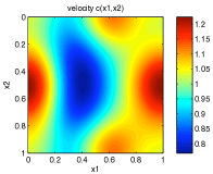
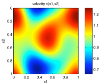
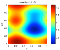
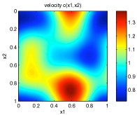
Figure 2: Some examples for the velocity $c$

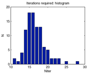
Figure 3: Histogram describing the number of iterations for convergence for $\omega=40\pi$ and 100 different choices of $c$.

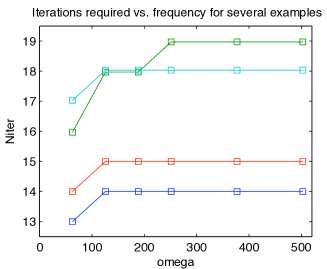
Figure 4: Number of iterations required vs. frequency for four choices of $c$ within the class described

7 Conclusion and discussion

We presented a preconditioning method for the multi-dimensional Helmholtz equation. The preconditioning was based on a frame of functions designed to have a special phase space tiling, adapted to the Helmholtz operator. The tiles follow to a certain degree the level sets of the absolute value of the symbol, they are of the general form

$$\bigcup_{x\in V}\{x\}\times\Xi(x).$$ (52)

Here $\Xi(x)$ is an $x$-dependent subset of the Fourier coordinate space, $V$ we chosen as a coordinate block. The tiles were curved because of the nontrivial dependence of $\Xi(x)$ on $x$.

Our main goal was to establish whether this kind of phase space tiling could be useful for preconditioning the Helmholtz equation. This is clearly shown by the numerical experiments. Apart from the convergence, a second important property was that a large part of the computations could be done on very coarse grids.

The generalization to 3-D would of course be of interest. A question is whether in 3-D the evaluation of the FIO in (48) can be speeded up by using the results of [4]. It is perhaps useful to point out some other directions for further development. One issue is the inclusion of boundary conditions. For applications like seismic imaging, the use of a simple absorbing boundary layers can be sufficient. The next step would be to include a boundary with Dirichlet or Neumann conditions at a planar or non-planar surface. Less smooth media are another interesting issue. We believe the results of this paper form a strong motivation for such further research.

References

- [1] S. Alinhac and P. Gérard. Pseudo-differential operators and the Nash-Moser theorem. American Mathematical Society, USA, 2007.
- [2] S. K. Bhowmik and C. C. Stolk. Preconditioners based on windowed fourier frames applied to elliptic partial differential equations. arXiv:1009.1925, 2010.
- [3] A. Brandt and I. Livshits. Wave-ray multigrid method for standing wave equations. Electron. Trans. Numer. Anal., 6(Dec.):162–181 (electronic), 1997. Special issue on multilevel methods (Copper Mountain, CO, 1997).
- [4] E. Candès, L. Demanet, and L. Ying. Fast computation of Fourier integral operators. SIAM J. Sci. Comput., 29(6):2464–2493 (electronic), 2007.
- [5] E. J. Candès and L. Demanet. The curvelet representation of wave propagators is optimally sparse. Comm. Pure Appl. Math., 58(11):1472–1528, 2005.
- [6] A. Cohen. Numerical analysis of wavelet methods, volume 32 of Studies in Mathematics and its Applications. North-Holland Publishing Co., Amsterdam, 2003.
- [7] A. Córdoba and C. Fefferman. Wave packets and Fourier integral operators. Comm. Partial Differential Equations, 3(11):979–1005, 1978.
- [8] W. Dahmen. Wavelet and multiscale methods for operator equations. In Acta Numerica, 1997, pages 55–228. Cambridge Univ. Press, Cambridge, 1997.
- [9] W. Dahmen, S. Prössdorf, and R. Schneider. Wavelet approximation methods for pseudodifferential equations. II. Matrix compression and fast solution. Adv. Comput. Math., 1(3-4):259–335, 1993.
- [10] J. J. Duistermaat. Fourier Integral Operators. Birkhäuser, Boston, 1996.
- [11] H. C. Elman, O. G. Ernst, and D. P. O’Leary. A multigrid method enhanced by Krylov subspace iteration for discrete Helmhotz equations. SIAM J. Sci. Comput., 23(4):1291–1315 (electronic), 2001.
- [12] B. Engquist and L. Ying. Sweeping preconditioner for the helmholtz equation: Hierarchical matrix representation. preprint, 2010. http://www.math.utexas.edu/users/lexing/publications/index.html.
- [13] B. Engquist and L. Ying. Sweeping preconditioner for the helmholtz equation: Moving perfectly matched layers. preprint, 2010. http://www.math.utexas.edu/users/lexing/publications/index.html.
- [14] Y. Erlangga, C. Oosterlee, and C. Vuik. A novel multigrid based preconditioner for heterogeneous Helmholtz problems. SIAM JOURNAL ON SCIENTIFIC COMPUTING, 27(4):1471–1492, 2006.
- [15] L. C. Evans. Partial differential equations, volume 19 of Graduate Studies in Mathematics. American Mathematical Society, Providence, RI, 1998.
- [16] C. Gérard and J. Sjöstrand. Semiclassical resonances generated by a closed trajectory of hyperbolic type. Comm. Math. Phys., 108(3):391–421, 1987.
- [17] B. Helffer and J. Sjöstrand. Résonances en limite semi-classique. Mém. Soc. Math. France (N.S.), (24-25):iv+228, 1986.
- [18] F. Hérau, J. Sjöstrand, and C. C. Stolk. Semiclassical analysis for the Kramers-Fokker-Planck equation. Comm. Partial Differential Equations, 30(4-6):689–760, 2005.
- [19] F. J. Herrmann, C. R. Brown, Y. A. Erlangga, and P. P. Moghaddam. Curvelet-based migration preconditioning and scaling (vol 74, pg A41, 2009). GEOPHYSICS, 74(6):Y9, NOV-DEC 2009.
- [20] F. J. Herrmann, P. Moghaddam, and C. C. Stolk. Sparsity- and continuity-promoting seismic image recovery with curvelet frames. Appl. Comput. Harmon. Anal., 24(2):150–173, 2008.
- [21] L. Hörmander. The Analysis of Linear Partial Differential Operators, volume 3. Springer-Verlag, Berlin, 1985.
- [22] L. Hörmander. The Analysis of Linear Partial Differential Operators, volume 4. Springer-Verlag, Berlin, 1985.
- [23] I. Livshits. An algebraic multigrid wave-ray algorithm to solve eigenvalue problems for the Helmholtz operator. Numer. Linear Algebra Appl., 11(2-3):229–239, 2004.
- [24] S. Mallat. A wavelet tour of signal processing. Elsevier/Academic Press, Amsterdam, third edition, 2009. The sparse way, With contributions from Gabriel Peyré.
- [25] A. Martinez. An introduction to semiclassical and microlocal analysis. Universitext. Springer-Verlag, New York, 2002.
- [26] T. J. P. M. Op ’t Root and C. C. Stolk. One-way wave propagation with amplitude based on pseudo-differential operators. Wave Motion, 47(2):67–84, 2010.
- [27] D. Osei-Kuffuor and Y. Saad. Preconditioning Helmholtz linear systems. APPLIED NUMERICAL MATHEMATICS, 60(4, Sp. Iss. SI):420–431, APR 2010.
- [28] J. Sjöstrand. Singularités analytiques microlocales. In Astérisque, 95, volume 95 of Astérisque, pages 1–166. Soc. Math. France, Paris, 1982.
- [29] H. F. Smith. A parametrix construction for wave equations with coefficients. Ann. Inst. Fourier (Grenoble), 48(3):797–835, 1998.
- [30] R. Stevenson. Adaptive solution of operator equations using wavelet frames. SIAM J. Numer. Anal., 41(3):1074–1100 (electronic), 2003.
- [31] M. E. Taylor. Pseudodifferential Operators. Princeton University Press, Princeton, New Jersey, 1981.
- [32] L. N. Trefethen and M. Embree. Spectra and pseudospectra. Princeton University Press, Princeton, NJ, 2005. The behavior of nonnormal matrices and operators.
- [33] F. Treves. Introduction to Pseudodifferential and Fourier Integral Operators, volume 2. Plenum Press, New York, 1980.