SPARSE CODING AND DICTIONARY LEARNING BASED ON THE MDL PRINCIPLE

Abstract

The power of sparse signal coding with learned dictionaries has been demonstrated in a variety of applications and fields, from signal processing to statistical inference and machine learning. However, the statistical properties of these models, such as underfitting or overfitting given sets of data, are still not well characterized in the literature. This work aims at filling this gap by means of the Minimum Description Length (MDL) principle – a well established information-theoretic approach to statistical inference. The resulting framework derives a family of efficient sparse coding and modeling (dictionary learning) algorithms, which by virtue of the MDL principle, are completely parameter free. Furthermore, such framework allows to incorporate additional prior information in the model, such as Markovian dependencies, in a natural way. We demonstrate the performance of the proposed framework with results for image denoising and classification tasks.

Index Terms—  Sparse coding, dictionary learning, MDL, denoising, classification

1 Introduction

Sparse models are by now well established in a variety of fields and applications, including signal processing, machine learning, and statistical inference, e.g. [1, 2, 3] and references therein.

When sparsity is a modeling device and not a hypothesis about the nature of the analyzed signals, parameters such as the desired sparsity in the solutions, or the size of the dictionaries to be learned, play a critical role in the effectiveness of sparse models for the tasks at hand. However, lacking theoretical guidelines for such parameters, published applications based on learned sparse models often rely on either cross-validation or ad-hoc methods for learning such parameters (an exception for example being the Bayesian approach, e.g., [4]) . Clearly, such techniques can be impractical and/or ineffective in many cases.

At the bottom of this problem lie fundamental questions such as: how rich or complex is a sparse model? how does this depend on the required sparsity of the solutions, or the size of the dictionaries? what is the best model for a given data class? A possible objective answer to such questions is provided by the Minimum Description Length principle (MDL) [5], a general methodology for assessing the ability of statistical models to capture regularity from data. The MDL principle is often regarded as a practical implementation of the Occam’s razor principle, which states that, given two descriptions for a given phenomenon, the shorter one is usually the best. In a nutshell, MDL equates “ability to capture regularity” with “ability to compress” the data, and the metric with which models are measured in MDL is codelength or compressibility.

The idea of using MDL for sparse signal coding was explored in the context of wavelet-based image denoising [6, 7]. These pioneering works were restricted to denoising using fixed orthonormal basis (wavelets). In addition, the underlying probabilistic models used to describe the transform coefficients, which are the main technical choice to make when applying MDL to a problem, were not well suited to the actual statistical properties of the modeled data (image encoding coefficients), thus resulting in poor performance. Furthermore, these works did not consider the critical effects of quantization in the coding, which needs to be taken into account when working in a true MDL framework (a useful model needs to be able to compress, that is, it needs to produce actual codes which are shorter than a trivial description of the data). Finally, these models are designed for noisy data, with no provisions for the important case of noiseless data modeling, which addresses the errors due to deviations from the model, and is critical in many applications such as classification.

The framework presented in this work addresses all of the above issues in a principled way: i) Efficient codes are used to describe the encoded data; ii) Deviations from the model are taken into account when modeling approximation errors, thus being more general and robust than traditional sparse models; iii) Probability models for (sparse) transform coefficients are corrected to take into account the high occurrence of zeros; iv) Quantization is included in the model, and its effect is treated rigorously; v) Dictionary learning is formulated in a way which is consistent with the model’s statistical assumptions. At the theoretical level, this brings us a step closer to the fundamental understanding of sparse models and brings a different perspective, that of MDL, into the sparse world. From a practical point of view, the resulting framework leads to coding and modeling algorithms which are completely parameter free and computationally efficient, and practically effective in a variety of applications.

Another important attribute of the proposed family of models is that prior information can be easily and naturally introduced via the underlying probability models defining the codelengths. The effect of such priors can then be quickly assessed in terms of the new codelengths obtained. For example, Markovian dependencies between sparse codes of adjacent image patches can be easily incorporated.

2 Background on sparse models

Assume we are given $n$ $m$-dimensional data samples ordered as columns of a matrix $\mathbf{{Y}}=[\mathbf{{y}}_{1}|\mathbf{{y}}_{2}|\ldots|\mathbf{{y}}_{n}]\in\mathbb{R}^{m{\times}n}$. Consider a linear model for $\mathbf{{Y}}$, $\mathbf{{Y}}=\mathbf{{D}}\mathbf{{A}}+\mathbf{{E}},$ where $\mathbf{{D}}=[\mathbf{{d}}_{1}|\mathbf{{d}}_{2}|\ldots|\mathbf{{d}}_{p}]$ is an $m{\times}p$ dictionary consisting of $p$ atoms, $\mathbf{{A}}=[\mathbf{{a}}_{1}|\mathbf{{a}}_{2}|\ldots|\mathbf{{a}}_{n}]\in\mathbb{R}^{p{\times}n}$ is a matrix of coefficients where each $j$-th column $\mathbf{{a}}_{j}$ specifies the linear combination of columns of $\mathbf{{D}}$ that approximates $\mathbf{{y}}_{j}$, and $\mathbf{{E}}=[\mathbf{{e}}_{1}|\mathbf{{e}}_{2}|\ldots|\mathbf{{e}}_{n}]\in\mathbb{R}^{m{\times}n}$ is a matrix of approximation errors. We say that the model is sparse if, for all or most $j=1,\ldots,n$, we can achieve $\left\|\mathbf{{e}}_{j}\right\|_{2}\approx 0$ while requiring that only a few coefficients $\gamma\ll p$ in $\mathbf{{a}}_{j}$ can be nonzero.

The problem of sparsely representing $\mathbf{{Y}}$ in terms of $\mathbf{{D}}$, which we refer to as the sparse coding problem, can be written as

$${\hat{\mathbf{{a}}}_{j}}\!=\!\arg\min_{\mathbf{{a}}}\left\|\mathbf{{a}}\right\|_{0}\!\quad\mathrm{s.t.}\quad\!\left\|\mathbf{{y}}_{j}\!-\!\mathbf{{D}}\mathbf{{a}}\right\|_{2}\leq\varepsilon,\;j=1,\ldots,n,$$ (1)

where $\left\|\mathbf{{a}}\right\|_{0}=\gamma$ is the pseudo-norm that counts the number of nonzero elements in a vector $\mathbf{{a}}$, and $\varepsilon$ is some small constant. There is a body of results showing that the problem (1), which is non-convex and NP-hard, can be solved exactly when certain conditions on $\mathbf{{D}}$ and $\mathbf{{A}}$ are met, by either well known greedy methods such as Matching Pursuit [8], or by solving a convex approximation to (1), commonly referred to as Basis Pursuit (BP) [9],

$$\hat{\mathbf{{a}}}_{j}=\arg\min_{\mathbf{{a}}}\left\|\mathbf{{a}}\right\|_{1}\!\!\quad\mathrm{s.t.}\quad\!\left\|\mathbf{{y}}_{j}-\mathbf{{D}}\mathbf{{a}}\right\|_{2}\leq\varepsilon,\;j=1,\ldots,n.$$ (2)

When $\mathbf{{D}}$ is included as an optimization variable, we refer to the resulting problem as sparse modeling. This problem is often written in unconstrained form,

$$(\hat{\mathbf{{D}}},\hat{\mathbf{{A}}})=\arg\min_{\mathbf{{D}},\mathbf{{A}}}\sum_{j=1}^{n}{\frac{1}{2}\left\|\mathbf{{y}}_{j}-\mathbf{{D}}\mathbf{{a}}_{j}\right\|_{2}^{2}+\lambda\left\|\mathbf{{a}}_{j}\right\|_{1}},$$ (3)

where $\lambda>0$ is an arbitrary constant. The problem in this case is non-convex in $(\mathbf{{D}},\mathbf{{A}})$, and one must be contempt with finding local minima. Despite this drawback, in recent years, models learned by (approximately) minimizing (3) have shown to be very effective for signal analysis, leading to state-of-the-art results in several applications such as image restoration and classification.

2.1 Model complexity of sparse models

In sparse modeling problems where $\mathbf{{D}}$ is learned, parameters such as the desired sparsity $\gamma$, the penalty $\lambda$ in (3), or the number of atoms $p$ in $\mathbf{{D}}$, must be chosen individually for each application and type of data to produce good results. In such cases, most sparse modeling techniques end-up using cross-validation or ad-hoc techniques to select these critical parameters. An alternative formal path is to postulate a Bayesian model where these parameters are assigned prior distributions, and such priors are adjusted through learning. This approach, followed for example in [4], adds robustness to the modeling framework, but leaves important issues unsolved, such as providing objective means to compare different models (with different priors, for example). The use of Bayesian sparse models implies having to repeatedly solve possibly costly optimization problems, increasing the computational burden of the applications.

In this work we propose to use the MDL principle to formally tackle the problem of sparse model selection. The goal is twofold: for sparse coding with fixed dictionary, we want MDL to tell us the set of coefficients that gives us the shortest description of a given sample. For dictionary learning, we want to obtain the dictionary which gives us the shortest average description of all data samples (or a representative set of samples from some class). A detailed description of such models, and the coding and modeling algorithms derived from them, is the subject of the next section.

3 MDL-based sparse coding and modeling framework

Sparse models break the input data $\mathbf{{Y}}$ into three parts: a dictionary $\mathbf{{D}}$, a set of coefficients $\mathbf{{A}}$, and a matrix of reconstruction errors. In order to apply MDL to a sparse model, one must provide codelength assignments for these components, $L(\mathbf{{A}})$, $L(\mathbf{{D}})$ and $L(\mathbf{{E}})$, so that the total codelength $L(\mathbf{{Y}})=L(\mathbf{{E}})+L(\mathbf{{A}})+L(\mathbf{{D}})$ can be computed. In designing such models, it is fundamental to incorporate as much prior information as possible so that no cost is paid in learning already known statistical features of the data, such as invariance to certain transformations or symmetries. Another feature to consider in sparse models is the predominance of zeroes in $\mathbf{{A}}$. In MDL, all this prior information is embodied in the probability models used for encoding each component. What follows is a description of such models.

Sequential coding– In the proposed framework, $\mathbf{{Y}}$ is encoded sequentially, one column $\mathbf{{y}}_{j}$ at a time, for $j=1,2,\ldots,n$, possibly using information (including dependencies) from previously encoded columns. However, when encoding each column $\mathbf{{y}}_{j}$, its sparse coefficients $\mathbf{{a}}_{j}$ are modeled as and IID sequence (of fixed length $p$).

Quantization– To achieve true compression, the finite precision of the input data $\mathbf{{Y}}$ must be taken into account. In the case of digital images for example, elements from $\mathbf{{Y}}$ usually take only $256$ possible values (from $0$ to $255$ in steps of size $\delta_{y}=1$). Since there is no need to encode $\mathbf{{E}}$ with more precision than $\mathbf{{Y}}$, we set the error quantization step to $\delta_{e}=\delta_{y}$. As for $\mathbf{{D}}$ and $\mathbf{{A}}$, the corresponding quantization steps $\delta_{a}$ and $\delta_{d}$ need to be fine enough to produce fluctuations on $\mathbf{{D}}\mathbf{{A}}$ which are smaller than the precision of $\mathbf{{Y}}$, but not more. Therefore, the actual distributions used are discretized versions of the ones discussed below.

Error– The elements of $\mathbf{{E}}$ are encoded with an IID model where the random value of a coefficient (represented by an r.v. $\epsilon$) is the linear superposition of two effects: $\epsilon=\hat{\epsilon}+\eta$, where $\eta\sim\mathcal{N}(0,\sigma^{2}_{\eta})$, $\sigma^{2}_{\eta}$ assumed known, models noise in $\mathbf{{Y}}$ due to measurement and/or quantization, and $\hat{\epsilon}\sim\mathcal{L}(0,\theta_{\epsilon})$ is a zero mean, heavy-tailed (Laplacian) error due to the model. The resulting distribution for $\epsilon$, which is the convolution of the involved Laplacian and Gaussian distributions, was developed in [10] under the name “LG.” This model will be referred to as $P_{\epsilon}(\cdot;\sigma^{2}_{\eta},\theta_{\epsilon})$ hereafter.

Sparse code– Each coefficient in $\mathbf{{A}}$ is modeled as the product of three (non-independent) random variables (see also [4] for a related model), $\alpha=\zeta\phi(\nu+\delta_{a})$, where $\zeta\sim\mathrm{Ber}(\rho)$ is a support indicator, that is, $\zeta=1$ implies $\alpha\neq 0$, $\phi=\mathrm{sgn}(\alpha)$, and $\nu=\max\{\left|\alpha\right|-\delta_{a},0\}$ is the absolute value of $\alpha$ corrected for the fact that $\nu\geq\delta_{a}$ when $\zeta=1$. Conditioned on $\zeta=0$, $\phi=\nu=0$ with probability $1$. Conditioned on $\zeta=1$, we assume $\phi\sim\mathrm{Ber}(1/2)$, and $\nu$ to be $\mathrm{Exp}(\theta_{\nu})$. Note that, with these choices, $P(\phi\nu|\zeta=1)$ is a Laplacian, which is a standard model for transform (e.g., DCT, Wavelet) coefficients. The probability models for the variables $\zeta$ and $\nu$ will be denoted as $P_{\zeta}(\cdot;\rho)$ and $P_{\nu}(\cdot;\theta_{\nu})$ respectively.

Dictionary– We assume the elements of $\mathbf{{D}}$ to be uniformly distributed on $[-1,1]$. Following the standard MDL recipe for encoding model parameter values learned from $n$ samples, we use a quantization step $\delta_{d}=n^{-1/2}$ [5]. For these choices we have $L(\mathbf{{D}})=mp\log_{2}n$, which does not depend on the element values of $\mathbf{{D}}$ but only on the number of atoms $p$ and the size of $\mathbf{{Y}}$. Other possible models which impose structure in $\mathbf{{D}}$, such as smoothness in the atoms, are natural to the proposed framework and will be treated in the extended version of this work.

3.1 Universal models for unknown parameters

The above probability models for the error $\epsilon$, support $\zeta$ and (shifted) coefficient magnitude $\nu$ depend on parameters which are not known in advance. In contrast with Bayesian approaches, cross-validation, or other techniques often used in sparse modeling, modern MDL solves this problem efficiently by means of the so called universal probability models [5]. In a nutshell, universal models provide optimal codelengths using probability distributions of a known family, with unknown parameters, thus generalizing the classic results from Shannon theory [11].

Following this, we substitute $P_{\zeta}(\cdot;\rho)$, $P_{\epsilon}(\cdot;\sigma^{2}_{\eta},\theta_{\epsilon})$ and $P_{\nu}(\cdot;\theta_{v})$ with corresponding universal models. For describing a given support $\mathbf{{z}}$, we use an enumerative code [12], which first describes the size of the support $\gamma$ with $\log_{2}p$ bits, and then the particular arrangement of non-zeros in $\mathbf{{z}}$ using $\log_{2}{p\choose\gamma}$ bits. $P_{\epsilon}(\cdot;\sigma^{2}_{\eta},\theta_{\epsilon})$ and $P_{\nu}(\cdot;\theta_{v})$ are substituted by corresponding universal mixture models, one of the possibilities dictated by the theory of universal modeling,

$$Q_{\epsilon}(u;\sigma^{2}_{\eta}) =\!\!\int_{0}^{+\infty}{\!\!\!\!\!\!\!\!w_{\epsilon}(\theta)P_{\epsilon}(u;\sigma^{2}_{\eta},\theta)d\theta},$$

$$Q_{\nu}(u) =\!\!\int_{0}^{+\infty}{\!\!\!\!\!\!\!\!w_{\nu}(\theta)P_{\nu}(u;\theta)d\theta},$$

where the mixing functions $w_{e}(\theta)$ and $w_{a}(\theta)$ are Gamma distributions (the conjugate prior for the exponential distribution), $w(\theta|\kappa,\beta)={\Gamma(\kappa)}^{-1}\theta^{\kappa-1}\beta^{\kappa}e^{-\beta\theta},\;\theta\in\mathbb{R}^{+}$ with fixed parameters $(\kappa_{\epsilon},\beta_{\epsilon})$ and $(\kappa_{\nu},\beta_{\nu})$ respectively. The resulting Mixture of Exponentials (MOE) distribution $Q_{\nu}(\cdot)$, is given by (see [13] for details), $Q_{\nu}(u|\beta_{\nu},\kappa_{\nu})=\kappa_{\nu}\beta_{\nu}^{\kappa_{\nu}}(u+\beta_{\nu})^{-(\kappa_{\nu}+1)},\;u\in\mathbb{R}^{+}.$ Observing that the convolution and the convex mixture operations that result in $Q_{\epsilon}(\cdot;\sigma^{2}_{\eta})$ are interchangeable (both integrals are finite), it turns out that $Q_{\epsilon}(\cdot;\sigma^{2}_{\eta})$ is a convolution of a MOE (of hyper-parameters $(\kappa_{\epsilon},\beta_{\epsilon})$) and a Gaussian with parameter $\sigma^{2}_{\eta}$. Thus, although the explicit formula for this distribution, which we call MOEG, is cumbersome, we can easily combine the results in [10] for the LG, and for MOE in [13] to perform tasks such as parameter estimation within this model. Note that the universality of these mixture models does not depend on the values of the hyper-parameters, and their choice has little impact on their overall performance. Here, guided by [13], we set $\kappa_{\nu}=\kappa_{\epsilon}=3.0$, $\beta_{\nu}=\beta_{\epsilon}=\delta_{a}$.

Following standard practice in MDL, the ideal Shannon code is used to translate probabilities into codelengths. Under this scheme, a sample value $u$ with probability $P(u)$ is assigned a code with length $L(u)=-\log P(u)$ (this is an ideal code because it only specifies a codelength, not a specific binary code, and because the codelengths produced can have a fractional number of bits). Then, for a given error residual $\mathbf{{e}}$ and coefficients magnitude vector $\mathbf{{v}}=[\max\{\left|a_{i}\right|-\delta_{a},0\}]_{i=1,\ldots,m}$, the respective ideal codelengths will be $L_{\epsilon}(\mathbf{{e}})=\!\sum_{i=1}^{m}{\!\!-\log_{2}Q_{\epsilon}(e_{i})}$ and $L_{\nu}(\mathbf{{v}})=\!\sum_{{k=1}\\ {\mathbf{{z}}_{k}=1}}^{p}{\!\!-\log_{2}Q_{\nu}(v_{k})}.$ Finally, following the assumed $\mathrm{Ber}(1/2)$ model, the sign of each non-zero element in $\mathbf{{a}}$ is encoded using 1 bit, for a total of $\gamma$ bits.

3.2 MDL-based sparse coding algorithms

The goal of a coding algorithm in this framework is to obtain, for each $j$-th sample $\mathbf{{y}}_{j}$, a vector $\mathbf{{a}}_{j}$ which minimizes its description,

$$\hat{\mathbf{{a}}}_{j}=\arg\min_{\mathbf{{a}}}L(\mathbf{{e}},\mathbf{{a}})=L_{\epsilon}(\mathbf{{e}}_{j})+L_{\zeta}(\mathbf{{z}})+L(\mathbf{{s}}|\mathbf{{z}})+L_{\nu}(\mathbf{{v}}|\mathbf{{z}}).$$ (4)

As it happens with most model selection algorithms, considering the support size ($\gamma=\left\|\mathbf{{a}}_{j}\right\|_{0}$) explicitly in the cost function results in a non-convex, discontinuous objective function. A common procedure in sparse coding for this case is to estimate the optimum support $\mathbf{{z}}_{j}^{\gamma}$ for each possible support size, $\gamma=1,2,\ldots,p$. Then, for each optimum support $\{\mathbf{{z}}_{j}^{\gamma}:\gamma\!=\!1,\ldots,p\}$, (4) is solved in terms of the corresponding non-zero values of $\mathbf{{a}}_{j}$, yielding a candidate solution $\mathbf{{a}}_{j}^{\gamma}$, and the one producing the smallest codelength is assigned to $\hat{\mathbf{{a}}}_{j}$. As an example of this procedure, we propose Algorithm 1, which is a variant of Matching Pursuit [8]. As in [8], we start with $\mathbf{{a}}_{j}^{0}=\mathbf{{0}}$, adding one new atom to the active set in each iteration. However, instead of adding the atom that is maximally correlated with the current residual $\mathbf{{e}}$ to the active set, we add the one yielding the largest decrease in overall codelength. The algorithm stops when no further decrease in codelength is obtained by adding a new atom.

An alternative for estimating $\{\mathbf{{z}}_{j}^{\gamma}:\gamma\!=\!1,\ldots,p\}$ is to use a convex model selection algorithm such as LARS/Lasso [14], which also begins with $\mathbf{{a}}_{j}^{0}=\mathbf{{0}}$, adding one atom at a time to the solution. For this case we propose to substitute the $\ell_{2}$ loss in LARS/Lasso by $-\log\mathrm{LG}(\cdot)$, which is more consistent with (4) and can be approximated by the Huber loss function [15]. This alternative will be discussed in detail in the extended version of this work.

Input: Data sample $\mathbf{{y}}$, dictionary $\mathbf{{D}}$

Output: The sparse code for $\mathbf{{y}}$, $\mathbf{{a}}$

initialize $\mathbf{{a}}\leftarrow\mathbf{{0}};\mathbf{{e}}\leftarrow\mathbf{{y}};L\leftarrow L(\mathbf{{0}});\;\mathbf{{z}}\leftarrow\mathbf{{0}}$ ;

initialize $\mathbf{{g}}\leftarrow\mathbf{{D}}^{T}\mathbf{{e}}$ ;  // correlation of current error with the dictionary

repeat for $k=1,\ldots,p:z_{k}=0$ do $\Delta_{k}\leftarrow[g_{k}]_{\delta_{a}}$ ;  // step $\Delta_{k}$ is correlation, quantized to prec. $\delta_{a}$

$L_{k}\leftarrow L(\mathbf{{a}}+\Delta_{k}\omega_{k})$ ;  // $\omega_{k}$ is the $k$-th canonical vector of $\mathbb{R}^{p}$

end Choose $\hat{k}=\arg\min_{k:z_{k}=0}\{L_{k}\}$;

if $L_{\hat{k}}<L$ then $L\leftarrow L_{\hat{k}}$ ;  // update current smallest codelength

$z_{\hat{k}}\leftarrow 1$ ;  // update support vector

$\mathbf{{a}}\leftarrow\mathbf{{a}}+\Delta_{\hat{k}}\omega_{\hat{k}}$ ;  // update coefficients vector

$\mathbf{{g}}\leftarrow\mathbf{{g}}-\Delta_{\hat{k}}\mathbf{{d}}_{\hat{k}}$ ;  // update correlation

end until $L_{\hat{k}}\geq L$ ;

Algorithm 1 Codelength-based Forward Selection.

3.3 Dictionary learning

Dictionary learning in the proposed framework proceeds in two stages. In the first one, a maximum dictionary size $p_{\mathrm{max}}$ is fixed and the algorithm learns $\mathbf{{D}}$ using alternate minimization in $\mathbf{{A}}$ and $\mathbf{{D}}$, as in standard dictionary learning approaches, now with the new codelength-based metric. First, $\mathbf{{D}}$ is fixed and $\mathbf{{A}}$ is updated as described in Section 3.2. Second, keeping $\mathbf{{A}}$ fixed, the update of $\mathbf{{D}}$ reduces to $\arg\min_{\mathbf{{D}}}L_{\epsilon}(\mathbf{{Y}}-\mathbf{{D}}\mathbf{{A}})$ (recall that $L(\mathbf{{D}})$ depends only on $p$, thus being constant at this stage). We add the constraint that $\left\|\mathbf{{d}}_{k}\right\|_{2}\leq 1,k=1,\ldots,p$, a standard form of dictionary regularization. Here too we approximate $L_{\epsilon}(\cdot)$ with the Huber function, obtaining a convex, differentiable dictionary update step which can be efficiently solved using scaled projected gradient. In practice, this function produces smaller codelengths than using standard $\ell_{2}$-based dictionary update, at the same computational cost (see Section 4).

In the second stage, the size of the dictionary is optimized by pruning atoms whose presence in $\mathbf{{D}}$ actually results in an increased average codelength. In practice, the final size of the dictionary reflects the intuitive complexity of the data to be modeled, thus validating the approach (see examples in Section 4).

4 Results and conclusion

The first experiment assesses that the learned models produce compressed descriptions of natural images. For this, we adapted a dictionary to the Pascal’06 image database, and encoded several of its images. The average bits per pixel obtained was $4.08$ bits per pixel (bpp), with $p=250$ atoms in the final dictionary. We repeated this using $\ell_{2}$ instead of Huber loss, obtaining $4.12$ bpp and $p=245$.

We now show example results obtained with our framework in two very different applications. In both cases we exploit spatial correlation between codes of adjacent patches by learning Markovian dependencies between their supports (see [16] for related work in the Bayesian framework). More specifically, we condition the probability of occurrence of an atom at a given position in the image, on the occurrence of that same atom in the left, top, and top-left patches. Note that, in both applications, the results were obtained without the need to adjust any parameter (although $\delta_{a}$ is a parameter of Algorithm 1, it was fixed beforehand to a value that did not introduce noticeable additional distortion in the model, and left untouched for the experiments shown here).

The first task is to estimate a clean image from an observed noisy version corrupted by Gaussian noise of known variance $\sigma^{2}_{\eta}$. Here $\mathbf{{Y}}$ contains all (overlapping) $8{\times}8$ patches from the noisy image. First, a dictionary $\mathbf{{D}}$ is learned from the noisy patches. Then each patch is encoded using $\mathbf{{D}}$ with a denoising variant of Algorithm 1, where the stopping criterion is changed for the requirement that the observed distortion falls within a ball of radius $\sqrt{m}\sigma_{\eta}$. Finally, the estimated patches are overlapped again and averaged to form the denoised image. From the results shown in Figure 1, it can be observed that adding a Markovian dependency between patches consistently improves the results. Note also that in contrast with [2], these results are fully parameter free, while those in [2] significantly depend on carefully tuned parameters.

The second application is texture segmentation via patch classification. Here we are given $c$ images with sample textures, and a target mosaic of textures, and the task is to assign each pixel in the mosaic to one of the textures. Again, all images are decomposed into overlapping patches. This time a dictionary $\mathbf{{D}}^{r}$ is learned for each texture $r=1,\ldots,c$ using the patches from the training images. Then, each patch in the mosaic is encoded using all available dictionaries, and its center pixel is assigned to the class which produced the shortest description length for that patch. The final result includes a simple $3{\times}3$ median filter to smooth the segmentation. We show a sample result in Figure 2. Here, again, the whole process is parameter free, and adding Markovian dependency improves the overall error rate ($7.5\%$ against $8.5\%$).

In summary, we have presented an MDL-based sparse modeling framework, which automatically adapts to the inherent complexity of the data at hand using codelength as a metric. As a result, the framework can be applied out-of-the-box to very different applications, obtaining competitive results in all the cases presented. We have also shown how prior information, such as spatial dependencies, are easily added to the framework by means of probability models.

noise $\rightarrow$	$\sigma_{\epsilon}=10$			$\sigma_{\epsilon}=20$
image $\downarrow$	IID	Markov	[2]	IID	Markov	[2]
lena	35.0	35.0	35.5	32.0	32.3	32.4
barbara	33.9	34.1	34.4	30.6	30.7	30.8
boats	32.9	32.9	33.6	30.1	30.2	30.3
peppers	34.0	34.0	34.3	31.4	31.5	30.8

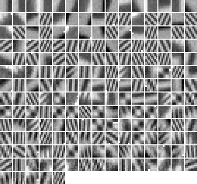
Fig. 1: Denoising results. Left to right: PSNR of denoised images for different methods and noise levels (including [2] as a reference), sample recovered patch from Barbara, best dictionary for Barbara ($p=200$, we used an initial $p_{\max}=512$).

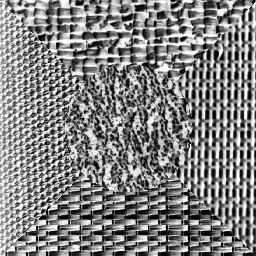
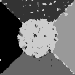
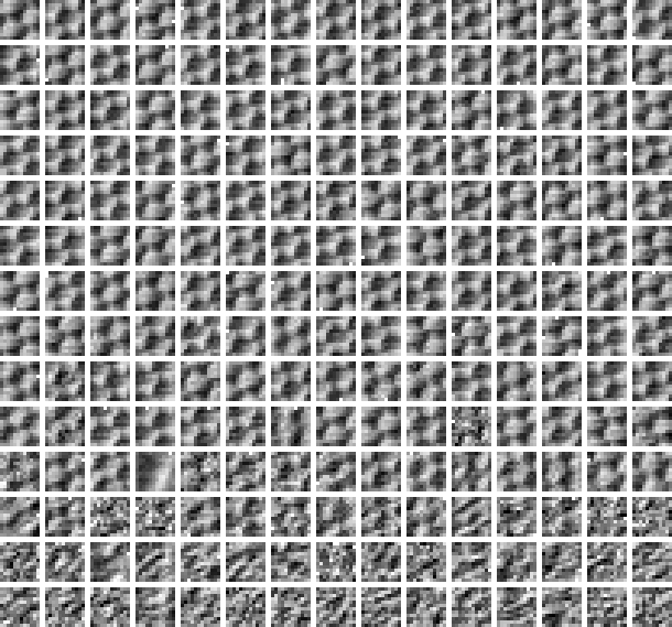
Fig. 2: Segmentation results. Left to right: sample “Nat-5c” taken from http://www.ux.uis.no/~tranden/data.html, obtained segmentation (error rate $7.5\%$), learned dictionaries for classes $1$ ($p_{1}=210$) and $2$ ($p_{2}=201$).

References

- [1] E. J. Candès, “Compressive sampling,” Proc. of the International Congress of Mathematicians, vol. 3, Aug. 2006.
- [2] M. Aharon, M. Elad, and A. Bruckstein, “The K-SVD: An algorithm for designing of overcomplete dictionaries for sparse representations,” IEEE Trans. SP, vol. 54, no. 11, pp. 4311–4322, Nov. 2006.
- [3] J. Mairal, M. Leordeanu, F. Bach, M. Hebert, and J. Ponce, “Discriminative sparse image models for class-specific edge detection and image interpretation,” in Proc. ECCV, Oct. 2008.
- [4] M. Zhou, H. Chen, J. Paisley, L. Ren, L. Li, Z. Xing, D. Dunson, G. Sapiro, and L. Carin, “Nonparametric bayesian dictionary learning for analysis of noisy and incomplete images,” submitted to IEEE Trans. Image Processing, 2011.
- [5] J. Rissanen, “Universal coding, information, prediction and estimation,” IEEE Trans. IT, vol. 30, no. 4, July 1984.
- [6] N. Saito, “Simultaneous noise suppression and signal compression using a library of orthonormal bases and the MDL criterion,” in Wavelets in Geophysics, E. Foufoula-Georgiou and P. Kumar, Eds., pp. 299––324. New York: Academic, 1994.
- [7] P. Moulin and J. Liu, “Statistical imaging and complexity regularization,” IEEE Trans. IT, Aug. 2000.
- [8] S. Mallat and Z. Zhang, “Matching pursuit in a time-frequency dictionary,” IEEE Trans. SP, vol. 41, no. 12, pp. 3397–3415, 1993.
- [9] S. Chen, D. Donoho, and M. Saunders, “Atomic decomposition by basis pursuit,” SIAM Journal on Scientific Computing, vol. 20, no. 1, pp. 33–61, 1998.
- [10] G. Motta, E. Ordentlich, I. Ramirez, G. Seroussi, and M. Weinberger, “The iDUDE framework for grayscale image denoising,” IEEE Trans. IP, vol. PP, no. 19, pp. 1–1, 2010, http://dx.doi.org/10.1109/TIP.2010.2053939.
- [11] T. Cover and J. Thomas, Elements of information theory, John Wiley and Sons, Inc., 2 edition, 2006.
- [12] T. M. Cover, “Enumerative source encoding,” IEEE Trans. IT, vol. 19, no. 1, pp. 73–77, 1973.
- [13] I. Ramírez and G. Sapiro, “Universal regularizers for robust sparse coding and modeling,” Submitted. Preprint available in arXiv:1003.2941v2 [cs.IT], August 2010.
- [14] B. Efron, T. Hastie, I. Johnstone, and R. Tibshirani, “Least angle regression,” Annals of statistics, vol. 32, no. 2, pp. 407–499, 2004.
- [15] P. J. Huber, “Robust estimation of a location parameter,” Annals of Statistics, vol. 53, pp. 73–101, 1964.
- [16] J. Paisley, M. Zhou, G. Sapiro, and L. Carin, “Nonparametric image interpolation and dictionary learning using spatially-dependent Dirichlet and beta process priors,” in IEEE ICIP, Sept. 2010.