Mesoscopic theory for inhomogeneous mixtures

Abstract

Mesoscopic density functional theory for inhomogeneous mixtures of sperical particles is developed in terms of mesoscopic volume fractions by a systematic coarse-graining procedure starting form microscopic theory. Approximate expressions for the correlation functions and for the grand potential are obtained for weak ordering on mesoscopic length scales. Stability analysis of the disordered phase is performed in mean-field approximation (MF) and beyond. MF shows existence of either a spinodal or a $\lambda$-surface on the volume-fractions - temperature phase diagram. Separation into homogeneous phases or formation of inhomogeneous distribution of particles occurs on the low-temperature side of the former or the latter surface respectively, depending on both the interaction potentials and the size ratios between particles of different species. Beyond MF the spinodal surface is shifted, and the instability at the $\lambda$-surface is suppressed by fluctuations. We interpret the $\lambda$-surface as a borderline between homogeneous and inhomogeneous (containing clusters or other aggregates) structure of the disordered phase. For two-component systems explicit expressions for the MF spinodal and $\lambda$-surfaces are derived. Examples of interaction potentials of simple form are analyzed in some detail, in order to identify conditions leading to inhomogeneous structures.

I Introduction

One of the main problems that arise in theoretical description of complex fluids is the role of density fluctuations on the mesoscopic length scale. Such fluctuations are not important in the case of simple fluids, and for this reason simple liquids can be accurately described by the liquid theories [1] which focus on the microscopic length scale, whereas the long-range fluctuations are treated via mean-field (MF) approximation. An exception is the critical region where the long-range fluctuations dominate. Universal features of the critical phenomena are described by the phenomenological Landau-Ginzburg-Wilson (LGW) theory [2, 3], because the field-theoretic methods allow for more accurate treatment of the dominant long-wavelength density fluctuations. In the LGW theory the microscopic structure is entirely neglected, however - the pair correlation function in the LGW theory decays monotonically. The two approaches (i) accurate description of the microscopic length scale and rough approximation for the long-wavelength fluctuations, and (ii) accurate description of the long-wavelength fluctuations with neglected microscopic structure are complementary. Both, used separately, give satisfactory description of simple fluids. Exact theories that are capable of description of nonuniversal features of phase transitions were also developed [4, 5, 6, 7, 8, 9], but so far these theories were applied to homogeneous phases.

When there are competing tendencies in the interaction potentials, then self-assembly into different aggregates, living polymers, clusters, micelles or another objects (’supermolecules’ having characteristic size) may occur. A notable example of such interactions is the effective short-range attraction long-range repulsion (SALR) potential [10, 11, 12, 13, 14, 15, 16]. In addition to the liquid order on the microscopic length scale (described by the pair distribution function) ordering on the mesoscopic length scale may be present in such systems. This additional ordering is associated with packing of the ’supermolecules’ in the lyotropic liquid crystalline phases. In the liquid theories, designed for description of the microscopic structure, the presence of such additional ordering is manifested by a lack of solutions of the associated equations [10, 13, 14, 15]. On the other hand, in the Landau theory modified by Brazovskii the dominant fluctuations of the order parameter (OP) are of finite wavelength [17]. The functional of the form postulated by Brazovskii was used for a description of various amphiphilic systems [18, 19, 20, 21, 22, 23], since the dominant finite-wavelength fluctuations of the abstract order parameter (OP) can represent in particular the density fluctuations on the mesoscopic length scale. Indeed, when the values of the phenomenological parameters in the functional are properly adjusted, the LB theory predicts stability (or metastability) of lyotropic liquid crystalline phases observed in amphiphilic systems [18, 20, 21, 22, 23]. One should note that in the LB theory fluctuations of the OP lead to a change of the continuous transition between disordered and lamellar phases obtained in MF to weakly first order transition [17] which occurs at lower temperature. The long-wavelength fluctuations in the LGW theory just modify the critical exponents, whereas the order of the transition remains the same. The Landau-Brazovskii (LB) functional is quite general (the OP can have different physical meaning), and is expressed in terms of phenomenological parameters (coupling constants) whose precise relation to measurable quantities is not known - it should be derived from more fundamental microscopic theory. Because the LB theory correctly describes the qualitative properties of systems self-assembling on the mesoscopic length scale, it is desirable to find a relation between the Brazovskii theory and the exact statistical mechanics. The main questions are: (i) what is the range of validity of the LGW and LB theories (ii) for what kind of interaction potentials the LB rather than the LGW theory is valid (iii) how the phenomenological parameters are expressed in terms of thermodynamic parameters and (effective) interaction potential. The approximate theory derived from the statistical mechanics should allow for determination of phase diagrams and structure when the interaction potentials are known.

A natural theory to start with is the density functional theory (DFT) [24] which allows for description of inhomogeneous systems and in principle is exact. However, the exact form of the grand potential functional is not known. In the widely used versions of the DFT the contribution to the grand potential associated with interactions is of the MF type. This approximation works well for a description of the microscopic structure and away from the critical point. However, more accurate approximation for the grand potential functional is desirable when the mesoscopic scale fluctuations dominate and may affect the order and location of the phase transition to a liquid crystalline phase. On the other hand, we have to make simplifying assumptions to make the theory tractable.

Since we need a description of the ordering on the mesoscopic length scale, we may introduce mesoscopic density that describes the distribution of particles less accurately than the microscopic density, but more accurately than the average density. Such an approach was proposed in Ref.[25] for a one component system of spherical particles. The mesoscopic density is defined as the microscopic density averaged over regions larger than the molecules and smaller than the characteristic length of ordering (for example, the size of the clusters). Precise definition is given for multicomponent systems in the next section. Probability of spontaneous appearance of particular mesoscopic density field was derived from the statistical mechanics by integrating the probability distribution over all microscopic states under the constraint of fixed mesoscopic density field under consideration. This method is analogous to integrating the probability distribution over all microscopic states under the constraint of fixed average density in macroscopic parts of the system. The only difference is that the constraint imposed on the microscopic density has a form of the field which varies on the mesoscopic length scale. The grand potential functional of the mesoscopic density field derived in Ref.[25] consists of two terms. The first term contains contributions from fluctuations on the microscopic length scale under the constraint of fixed mesoscopic density $\bar{\rho}({\bf r})$. This term resembles standard DFT. The second contribution is associated with mesoscopic fluctuations $\phi({\bf r})$ that can occur in the system when the constraint $\bar{\rho}({\bf r})$ is removed.

In the MF approximation the contribution to the grand potential associated with mesoscopic-length scale fluctuations is neglected. In this version of MF the average density is approximated by the most probable mesoscopic density [25]. However, in parts of the phase diagram that are close to microphase separation the fluctuation contribution can be comparable to the first term, and the average density can be significantly different from the most probable mesoscopic density. In such cases the fluctuations cannot be neglected.

It is worthwhile to note that the relation between the systems with and without the constraint on the mesoscopic density distribution resembles the relation between the canonical and the grand canonical ensembles. There is some loose analogy between the system in the presence of the mesoscopic constraint imposed on the microscopic density distribution, and a macroscopic system with fixed number of particles $N=N_{0}$, described by the canonical ensemble. When the constraint of compatibility between the microscopic density distribution and the mesoscopic field $\bar{\rho}({\bf r})$ is removed and $\langle\phi({\bf r})\rangle=0$, then the system is analogous to the open system with fluctuating $N$ such that $\langle N\rangle=N_{0}$ (grand canonical ensemble). The canonical and grand canonical ensembles with $N_{0}=\langle N\rangle$ are equivalent only far from phase transitions, when the fluctuations are small, $\langle(N-N_{0})^{2}\rangle\propto\chi_{T}N_{0}$. Close to phase transitions the compressibility $\chi_{T}$ is large (diverges at the transition), and fluctuations cannot be neglected. At the phase coexistence the most probable density distribution in the open system corresponds to either the gas $\rho_{g}$ or the liquid $\rho_{l}$ density in an absence of any constraints or external fields. However, in the grand canonical ensemble the ensemble average in an absence of any constraints or external fields yields a constant density $(\rho_{g}+\rho_{l})/2$, although homogeneous microscopic states with such density occur with negligible probability. The difference between this case and microphase separation concerns the extent of the regions having different density (or composition) - mesoscopic rather than macroscopic parts of the system - and in turn the time scale associated with displacements of these regions, i.e. with the mesoscopic rather than macroscopic fluctuations. While it is justified to neglect macroscopic fluctuations in studies of coexisting homogeneous phases, in the case of microphase separation the mesoscopic fluctuations influence the experimentally observed properties of the system.

The fluctuation contribution to the grand potential reduces to the form similar to the LB theory in the case of weak ordering on the length scale significantly larger than the molecular size [25]. Such kind of ordering occurs in soft-matter systems, and the results of Ref. [25] confirm validity of the LB theory for soft matter. The fluctuation contribution can be treated by field-theoretic methods, and in the theory developed in Ref.[25] the DFT and field-theoretic methods are both used.

The theory developed in Ref.[25] is restricted to a one-component system, whereas the soft-matter systems are usually multicomponent. The size of solvent molecules can be several orders of magnitude smaller than the size of proteins, nanoparticles or colloids, and the solvent molecules can be taken into account only via solvent-mediated effective interactions between solute particles [26, 27]. However, the effectively one-component system might lead to incorrect predictions when the size ratio is not very large, and when mesoscopic fluctuations of the solvent are important. The purpose of this work is an extension of the mesoscopic DFT to the case of multicomponent systems of particles of arbitrary sizes.

In sec.2 general framework of the theory for multicomponent systems is introduced by a systematic coarse-graining procedure. Mesoscopic volume fractions are defined, and expressions for the grand potential and correlation functions are derived in the same section. In sec.3 approximate theory for weak ordering is developed, and the role of mesoscopic fluctuations for stability of the disordered phase is discussed. Two-component systems of particles of different sizes are studied in more detail in sec.4. The MF theory is illustrated by three simple examples. Equations derived in sec.4 are of MF type, and provide information whether inhomogeneities on the mesoscopic length scale (clusters or soft crystals) are formed, or the system can phase separate into homogeneous phases for given interaction potentials and size ratios. In future studies the theory can be applied to different inhomogeneous systems along the lines described in sec.3.

II Coarse graining

II.1 microscopic density and microscopic volume fraction

We consider an $n$-component mixture of nearly spherical particles, with the components labeled by Greek letters. The diameter of the hard core of the particle of the specie $\alpha$ is denoted by $\sigma_{\alpha}$. A microscopic state is defined by the positions of the centers of mass of $N_{1},...,N_{n}$ particles,

$${\cal M}=\{\{{\bf r}^{\alpha}_{i}\}_{i=1,...,N_{\alpha}},\alpha=1,...,n\}$$ (1)

where ${\bf r}^{\alpha}_{i}$ denotes the position of the $i$-th particle of the $\alpha$-th specie, and $N_{\alpha}$ denotes the number of particles of the $\alpha$-th specie in the considered microstate. Microscopic density of the $\alpha$-th specie is given by the standard definition,

$$\hat{\rho}_{\alpha}({\bf r},{\cal M}):=\sum_{i=1}^{N_{\alpha}}\delta({\bf r}-{\bf r}_{i}^{\alpha}).$$ (2)

For particles of different sizes, for example for a mixture of nanoparticles and small molecules, it is convenient to introduce microscopic density that takes into account distribution of matter inside the molecules, and instead of (2) we introduce

$$\hat{\zeta}_{\alpha}({\bf r},{\cal M}):=\sum_{i=1}^{N_{\alpha}}f_{\alpha}(|{\bf r}-{\bf r}_{i}^{\alpha}|)$$ (3)

where spherically-symmetric structure of molecules is assumed, $\int_{\bf r}f_{\alpha}(r)=v_{\alpha}$ with $v_{\alpha}=\pi\sigma_{\alpha}^{3}/6$ denoting the volume of the particle of the specie $\alpha$, and $f_{\alpha}(r)$ describes distribution of matter inside such particle at the distance $r$ from its center. For brevity we shall use the notation $\int_{\bf r}\equiv\int d{\bf r}$, indicating the integration region $S$ by $\int_{{\bf r^{\prime}}\in S}$ when necessary. For constant density inside the particle Eq.(3) reduces to the microscopic volume fraction defined by

$$\hat{\zeta}_{\alpha}({\bf r},{\cal M}):=\sum_{i=1}^{N_{\alpha}}\theta\Big{(}\frac{\sigma_{\alpha}}{2}-|{\bf r}-{\bf r}_{i}^{\alpha}|\Big{)}$$ (4)

where $\theta(r)$ is the Heaviside unit step function. Integration of $\hat{\zeta}_{\alpha}({\bf r},{\cal M})$ over the system volume gives the volume occupied by the particles. The interaction energy for a pair of particles $i,j$ of the $\alpha$, $\beta$ species with the centers at ${\bf r}_{i}^{\alpha}$ and ${\bf r}_{j}^{\beta}$ respectively is

$$U_{\alpha\beta}(|{\bf r}_{i}^{\alpha}-{\bf r}_{j}^{\beta}|)=\int_{\bf r}\int_{\bf r^{\prime}}f_{\alpha}(|{\bf r}-{\bf r}_{i}^{\alpha}|)V_{\alpha\beta}({\bf r},{\bf r}^{\prime})f_{\beta}(|{\bf r}^{\prime}-{\bf r}_{j}^{\beta}|).$$ (5)

Summation convention for repeated Greek indexes is assumed above and in the whole article. $V_{\alpha\beta}({\bf r},{\bf r}^{\prime})d{\bf r}d{\bf r^{\prime}}$ is the interaction potential between the infinitesimal volumes $d{\bf r}$ and $d{\bf r^{\prime}}$ around the points ${\bf r}$ and ${\bf r^{\prime}}$ inside the particles $\alpha$ and $\beta$. The energy of the system in the microstate defined by (3) or (2) can be written as

$$E[{\cal M}]=\frac{1}{2}\int_{\bf r}\int_{\bf r^{\prime}}\hat{\zeta}_{\alpha}({\bf r},{\cal M})V_{\alpha\beta}({\bf r},{\bf r}^{\prime})\hat{\zeta}_{\beta}({\bf r}^{\prime},{\cal M})$$ (6)

$$=\frac{1}{2}\sum_{\alpha=1}^{n}\sum_{\beta=1}^{n}\sum_{i=1}^{N_{\alpha}}\sum_{j=1}^{N_{\beta}}U_{\alpha\beta}(|{\bf r}_{i}^{\alpha}-{\bf r}_{j}^{\beta}|)$$

$$=\frac{1}{2}\int_{\bf r}\int_{\bf r^{\prime}}\hat{\rho}_{\alpha}({\bf r},{\cal M})U_{\alpha\beta}({\bf r},{\bf r}^{\prime})\hat{\rho}_{\beta}({\bf r}^{\prime},{\cal M})$$

II.2 Mesoscopic density and mesoscopic volume fraction

Let us choose the mesoscopic length scale $R$ and consider spheres $S_{R}({\bf r})$ of radius $R$ and centers at ${\bf r}$ that cover the whole volume $V$ of the system. In order to describe ordering on the length scale $\lambda$, we should choose $R<\lambda$. We define the mesoscopic density of the specie $\alpha$ by an extension of the definition introduced for a one-component system in Ref.[25]

$$\rho_{\alpha}({\bf r}):=\frac{1}{V_{S}}\int_{{\bf r^{\prime}}\in S_{R}({\bf r})}\hat{\rho}_{\alpha}({\bf r^{\prime}},{\cal M}),$$ (7)

where $V_{S}=4\pi R^{3}/3$ is the volume of the sphere $S_{R}({\bf r})$. Similarly, the mesoscopic volume fraction of the specie $\alpha$ at ${\bf r}$ is defined by

$$\zeta_{\alpha}({\bf r}):=\frac{1}{V_{S}}\int_{{\bf r^{\prime}}\in S_{R}({\bf r})}\hat{\zeta}_{\alpha}({\bf r^{\prime}},{\cal M}).$$ (8)

For an illustration, the mesoscopic density and the mesoscopic volume fraction are shown in Fig. 1 for a one-component system, when a single particle is located at ${\bf r}={\bf 0}$, for three different mesoscopic length scales $R$. In this case the center of the particle is inside (outside) the sphere $S_{R}({\bf r})$ for $r<2R/\sigma_{\alpha}$ ($r>2R/\sigma_{\alpha}$), therefore for $r=2R/\sigma_{\alpha}$ the number density (7) has a discontinuity (Fig.2). For increasing length scale of coarse-graining, the difference between $\zeta$ and $\rho v$ decreases.

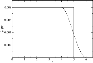
Figure 1: One-component system and the microstate in which a single hard sphere of a radius $\sigma/2$ is located at ${\bf r}={\bf 0}$ is considered for different length scales of coarse-graining. The mesoscopic volume-fraction $\zeta$ defined in Eq.(8) is shown by the dashed lines, and $\rho v$ is shown by the solid lines. $v=\pi\sigma^{3}/6$ and $\rho$ is defined in Eq.(7) (based on the standard definition of the microscopic density (2)). Top panel: $2R/\sigma=1$. Central panel: $2R/\sigma=2$. Bottom panel: $2R/\sigma=5$. In this particularly simple case the fields (8) and (7) are functions of the distance $r$ from the center of the hard sphere. In each case $\int_{\bf r}\zeta({\bf r})=v$. The distance $r$ is in $\sigma/2$ units, $\zeta$ and $\rho v$ are dimensionless.

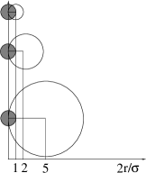
Figure 2: Cartoon showing distances corresponding to the discontinuities of the mesoscopic number density for different scales of coarse graining. From top to bottom $2R/\sigma=1$, $2R/\sigma=2$ and $2R/\sigma=5$, as in Fig.1. Shaded circle represents the particle located at ${\bf r=0}$, open circles represent the spheres $S_{R}({\bf r})$ with the centers at ${\bf r}$ over which the density or volume fraction is averaged. The mesoscopic density at the point ${\bf r}$ is the number of centers of particles inside the sphere $S_{R}({\bf r})$ divided by $4\pi R^{3}/3$. The mesoscopic volume fraction is the fraction of the volume $4\pi R^{3}/3$ that is occupied by the particles.

For a chosen length scale $R$ the mesostate can be defined by $\{\zeta\}=\{\zeta_{1}({\bf r}),...,\zeta_{n}({\bf r})\}$ or by $\{\rho\}=\{\rho_{1}({\bf r}),...,\rho_{n}({\bf r})\}$. Note that Eq.(7) or Eq.(8) describes a constraint imposed on the microscopic states, and $\{\zeta\}$ is equivalent to the constraint (8) imposed on all the components. For a chosen length scale $R$ all microscopic states can be separated into disjoint subsets, such that the microstates belonging to a particular subset are compatible with the same constraint (Eq.(8)). Microstates belonging to different subsets are compatible with different constraints, i.e. with a different form of $\{\zeta\}$ or $\{\rho\}$.

Probability density of a spontaneous occurrence of the mesostate $\{\zeta\}$ is given by

$$p[\{\zeta\}]={\Xi}^{-1}e^{-\beta\Omega_{co}[\{\zeta\}]}$$ (9)

where

$$\Xi=\int^{{}^{\prime}}D\zeta_{1}...\int^{{}^{\prime}}D\zeta_{n}e^{-\beta\Omega_{co}[\{\zeta\}]}.$$ (10)

and

$$e^{-\beta\Omega_{co}[\{\zeta\}]}=\int_{{\cal M}\in\{\{\zeta\},R\}}e^{-\beta(E[{\cal M}]-\int_{\bf r}\bar{\mu}_{\alpha}\zeta_{\alpha}({\bf r}))}.$$ (11)

$E[{\cal M}]$ is the microscopic Hamiltonian, and $\int_{{\cal M}\in\{\{\zeta\},R\}}$ is a symbolic notation for the integration over all microstates compatible with $\{\zeta\}$ according to Eq.(8). $\bar{\mu}_{\alpha}=\mu_{\alpha}/v_{\alpha}$ and $T$ are the chemical potential of the specie $\alpha$ (in appropriate units) and temperature respectively, and $\beta=1/k_{B}T$, with $k_{B}$ denoting the Boltzmann constant. $\Omega_{co}[\{\zeta\}]$ is the grand potential in the presence of the constraints $\{\zeta\}$ (Eq.(8)) imposed on the system. The functional integral $\int^{{}^{\prime}}D\zeta_{1}...\int^{{}^{\prime}}D\zeta_{n}$ in Eq.(10) is over all mesostates $\{\zeta\}$, which is indicated by the prime. In analogous way we can consider mesoscopic theory based on the mesoscopic density.

We obtain a mesoscopic theory with the same structure as the standard statistical mechanics. The integration over all microstates is replaced in Eq.(10) by the integration over all mesostates. The Hamiltonian is replaced in Eq.(9) and (10) by the grand potential in the presence of the constraint of compatibility with the given mesostate that is imposed on the microstates. The above formulas are exact. So far we just rearranged the summation over microstates. The reason for doing so is the possibility of performing the summation over the mesostates and over the microstates compatible with a particular mesostate by different methods.

Grand potential in the presence of the mesoscopic constraint can be written in the form

$$\Omega_{co}=U-TS-\mu_{\alpha}N_{\alpha},$$ (12)

where $U,S$ and $N_{\alpha}$ are the internal energy, entropy and the number of molecules of the specie $\alpha$ respectively in the system with the constraint (8) imposed on the microscopic densities. $U$ is given by the expression

$$U[\{\zeta\}]=\frac{1}{2}\int_{\bf r_{1}}\int_{\bf r_{2}}V_{\alpha\beta}^{co}({\bf r}_{1}-{\bf r}_{2})\zeta_{\alpha}({\bf r}_{1})\zeta_{\beta}({\bf r}_{2})=\frac{1}{2}\int_{\bf r_{1}}\int_{\bf r_{2}}U_{\alpha\beta}^{co}({\bf r}_{1}-{\bf r}_{2})\rho_{\alpha}({\bf r}_{1})\rho_{\beta}({\bf r}_{2}),$$ (13)

where

$$V_{\alpha\beta}^{co}({\bf r}_{1}-{\bf r}_{2})=V_{\alpha\beta}(r_{12})g_{\alpha\beta}^{\zeta co}({\bf r}_{1}-{\bf r}_{2})$$ (14)

$r_{12}=|{\bf r}_{1}-{\bf r}_{2}|$, and

$$g_{\alpha\beta}^{\zeta co}({\bf r}_{1}-{\bf r}_{2})=\frac{\langle\hat{\zeta}_{\alpha}({\bf r}_{1})\hat{\zeta}_{\beta}({\bf r}_{2})\rangle}{\zeta_{\alpha}({\bf r}_{1})\zeta_{\beta}({\bf r}_{2})}$$ (15)

is the microscopic pair correlation function for the volume fraction, in the presence of the constraint (8) imposed on the microscopic states. $U_{\alpha\beta}^{co}({\bf r}_{1}-{\bf r}_{2})$ is given by an expression analogous to Eq.(14), with $g_{\alpha\beta}^{\zeta co}$ replaced by $g_{\alpha\beta}^{co}$, the standard pair correlation function in the presence of the constraint (7). Note that the above functions differ from each other. In particular, for $g_{\alpha\beta}^{\zeta co}$ smooth increase from zero is expected for $r_{12}$ increasing from zero, whereas the correlation function for the microscopic density (Eq. (2)) vanishes for $r_{12}<\sigma_{\alpha\beta}$.

The advantage of $\zeta_{\alpha}({\bf r})$ is its continuity (see Fig.1). In addition, $\zeta_{\alpha}({\bf r})\leq\zeta_{cp}$ for all ${\bf r}$, where $\zeta_{cp}$ is the close-packing volume fraction, and the gradient of $\zeta$ is small, $|\nabla\zeta|<1/R$. The disadvantage of $\zeta_{\alpha}({\bf r})$ is the expression for the energy (13) in terms of the pair correlation function for the volume fraction, Eq.(15), which was not studied. The mesoscopic density (7) has discontinuities (see Fig.1), and for significantly different sizes of particles the number densities for different components may differ by several orders of magnitude. On the other hand, the expression for the energy (13) has a standard form in terms of the well known correlation function. When the ordering occurs on the length scale significantly larger than the size of the particles, we can make the approximation (see Fig.1)

$$\zeta_{\alpha}({\bf r})\approx\rho_{\alpha}({\bf r})v_{\alpha}.$$ (16)

Inserting the above expression for $\rho_{\alpha}$ into Eq.(13), yields

$$V^{co}_{\alpha\beta}({\bf r},{\bf r}^{\prime})\approx\frac{U^{co}_{\alpha\beta}({\bf r},{\bf r}^{\prime})}{v_{\alpha}v_{\beta}}.$$ (17)

It is important to remember that the approximation (17) is only valid when the ordering occurs on the length scale significantly larger than the size of particles.

We further assume that the entropy $S$ satisfies the relation $-TS=F_{h}$, where $F_{h}$ is the free-energy of the hard-sphere reference system with the constraint (8) imposed on the microscopic volume fractions.

II.3 Grand-potential functional and mesoscopic correlation functions

Let us introduce external fields $\{J\}=\{J_{1}({\bf r}),...,J_{n}({\bf r})\}$ and the grand-thermodynamic potential functional

$$\Omega[\{\beta J\}]:=-k_{B}T\log\Big{[}\int^{{}^{\prime}}D\zeta_{1}...\int^{{}^{\prime}}D\zeta_{n}e^{-\beta[\Omega_{co}[\{\zeta\}]-\int_{\bf r}J_{\alpha}({\bf r})\zeta_{\alpha}({\bf r})]}\Big{]}.$$ (18)

$-\beta\Omega[\beta J]$ is the generating functional for the (connected) correlation functions for the mesoscopic volume fractions,

$$\langle\zeta_{\alpha_{1}}({\bf r}_{1})...\zeta_{\alpha_{n}}({\bf r}_{n})\rangle^{con}=\frac{\delta^{n}(-\beta\Omega[\beta J])}{\delta(\beta J_{\alpha_{1}}({\bf r}_{1}))...\delta(\beta J_{\alpha_{n}}({\bf r}_{n}))}.$$ (19)

We introduce the notation

$$G^{m}_{\alpha\beta}({\bf r}_{1}-{\bf r}_{2})=\langle\zeta_{\alpha}({\bf r}_{1})\zeta_{\beta}({\bf r}_{2})\rangle^{con}=\langle\zeta_{\alpha}({\bf r}_{1})\zeta_{\beta}({\bf r}_{2})\rangle-\langle\zeta_{\alpha}({\bf r}_{1})\rangle\langle\zeta_{\beta}({\bf r}_{2})\rangle.$$ (20)

The relation between the mesoscopic and the microscopic correlation functions resulting from the definition of the mesoscopic volume fraction (8) is given by

$$\langle\zeta_{\alpha_{1}}({\bf r}_{1})\cdot...\cdot\zeta_{\alpha_{n}}({\bf r}_{n})\rangle$$ (21)

$$=\frac{\int^{{}^{\prime}}D\zeta_{1}...\int^{{}^{\prime}}D\zeta_{n}e^{-\beta[\Omega_{co}[\{\beta J\}]-\int_{\bf r}J_{\alpha}({\bf r})\zeta_{\alpha}({\bf r})]}\zeta_{\alpha_{1}}({\bf r}_{1})\cdot...\cdot\zeta_{\alpha_{n}}({\bf r}_{n})}{\int^{{}^{\prime}}D\zeta_{1}...\int^{{}^{\prime}}D\zeta_{n}e^{-\beta[\Omega_{co}[\{\beta J\}]-\int_{\bf r}J_{\alpha}({\bf r})\zeta_{\alpha}({\bf r})]}}$$

$$=\frac{1}{V_{S}}\int_{{\bf r^{\prime}}\in S_{R}({\bf r}_{1})}...\frac{1}{V_{S}}\int_{{\bf r^{(n)}}\in S_{R}({\bf r}_{n})}\langle\hat{\zeta}_{\alpha_{1}}({\bf r}^{\prime})\cdot...\cdot\hat{\zeta}_{\alpha_{n}}({\bf r}^{(n)})\rangle,$$

with analogous relation for the correlation functions for the microscopic and the mesoscopic densities. Note the difference between the micro- and the mesoscopic correlation functions resulting from the integration of the former over mesoscopic volumes. In particular, for $2R>\sigma_{\alpha\beta}$ the mesoscopic two-point correlation function for densities, analogous to Eq.(21), does not vanish for ${\bf r}_{1}={\bf r}_{2}$. This is because for ${\bf r}^{\prime}\in S_{R}({\bf r}_{1})$ and ${\bf r}^{\prime\prime}\in S_{R}(({\bf r}_{1})$, such that $|{\bf r}^{\prime}-{\bf r}^{\prime\prime}|>\sigma_{\alpha\beta}$, the corresponding microscopic correlation function on the RHS of an equation analogous to Eq.(21) does not vanish and contributes to the integral. We should stress that in Ref.[25] the theory is based on the mesoscopic density, but for significantly different sizes of particles the volume fraction is more convenient, as discussed in the previous subsection.

Let us introduce the Legendre transform

$$\beta F[\{\bar{\zeta}\}]:=\beta\Omega[\{\beta J\}]+\int_{\bf r}\beta J_{\alpha}({\bf r})\bar{\zeta}_{\alpha}({\bf r})$$ (22)

where

$$\bar{\zeta}_{\alpha}({\bf r})=\frac{\delta(-\beta\Omega)}{\delta(\beta J_{\alpha}({\bf r}))}$$ (23)

is the average field (volume fraction) for given $\{J\}$. The equation of state takes the form

$$\frac{\delta(\beta F)}{\delta\bar{\zeta}_{\alpha}({\bf r})}=\beta J_{\alpha}({\bf r}).$$ (24)

In general $\bar{\zeta}$ may differ from any mesostate defined in Eq.(8). We extend the functional $\Omega_{co}$ beyond the set of the mesostates. Let the extension be defined in Eq.(12) on the Hilbert space of fields that fulfill the restrictions following from the properties of the mesostates, and let us keep the notation $\Omega_{co}$ for this extension. The key restriction on the mesoscopic volume fraction is the magnitude and the gradient. In Fourier representation we shall consider the functions that vanish for $k>\pi/R$, where $k$ is the wave number. As discussed in Ref.[25], the fields with magnitudes exceeding the close packing (such fields belong to the Hilbert space, but do not represent any mesostate) are irrelevant, since the corresponding Boltzmann factor is very small. We introduce the functional $\beta F[\{\zeta\}]$ of the form

$$\beta F[\{\zeta\}]=\beta\Omega_{co}[\{\zeta\}]-\log\Big{[}\int D\phi_{1}...\int D\phi_{n}e^{-\beta[H_{fluc}-\int_{\bf r}J_{\alpha}({\bf r})\phi_{\alpha}({\bf r})]}\Big{]},$$ (25)

where $\phi_{\alpha}({\bf r})$ is the local fluctuation of the volume fraction of the component $\alpha$, and

$$H_{fluc}[\{\zeta\},\{\phi\}]=\Omega_{co}[\{\zeta+\phi\}]-\Omega_{co}[\{\zeta\}].$$ (26)

We introduced the notation $\{\phi\}=\{\phi_{1}({\bf r}),...,\phi_{n}({\bf r})\}$. From Eqs.(22) and (18) it follows that the functional (25) equals the grand potential, when $\{\zeta\}=\{\bar{\zeta}\}$, with $\{\bar{\zeta}\}$ determined from Eq.(24). By definition $\langle\phi_{\alpha}\rangle=0$ when $\{\zeta\}=\{\bar{\zeta}\}$.

Note that from Eq.(25) it follows that the inverse correlation functions (related to the direct correlation functions) defined by

$$C^{m}_{\alpha_{1},...\alpha_{n}}({\bf r}_{1},...,{\bf r}_{n})=\frac{\delta^{n}\beta F[\{\bar{\zeta}\}]}{\delta\bar{\zeta}_{\alpha_{1}}({\bf r}_{1})...\delta\bar{\zeta}_{\alpha_{n}}({\bf r}_{n})}$$ (27)

consist of two terms: the first one is the contribution from the fluctuations on the microscopic length scale ($<R$) with frozen fluctuations on the mesoscopic length scale. This term is

$${\cal C}^{co}_{\alpha_{1},...\alpha_{n}}({\bf r}_{1},...,{\bf r}_{n})=\frac{\delta^{n}\beta\Omega_{co}[\{\bar{\zeta}\}]}{\delta\bar{\zeta}_{\alpha_{1}}({\bf r}_{1})...\delta\bar{\zeta}_{\alpha_{n}}({\bf r}_{n})}.$$ (28)

The second term is the contribution from the fluctuations on the mesoscopic length scale ($>R$). From Eqs. (18)-(27) we obtain equations relating the inverse correlation functions with the many-body correlation functions. In the lowest nontrivial order beyond the mean-field approximation and for $J_{\alpha}=0$ we obtain (see [25])

$$\frac{\delta\beta\Omega_{co}[\{\bar{\zeta}\}]}{\delta\bar{\zeta}_{\alpha}({\bf r})}+\int_{\bf r_{1}}\int_{\bf r_{2}}G^{m}_{\alpha_{1}\alpha_{2}}({\bf r}_{1},{\bf r}_{2}){\cal C}_{\alpha_{1}\alpha_{2}}^{co}({\bf r}_{1},{\bf r}_{2},{\bf r})=0,$$ (29)

and

$$2C^{m}_{\alpha\beta}({\bf r}_{1},{\bf r}_{2})={\cal C}_{\alpha\beta}^{co}({\bf r}_{1},{\bf r}_{2})+\langle\frac{\delta^{2}(\beta H_{fluc})}{\delta\zeta_{\alpha}({\bf r}_{1})\delta\zeta_{\beta}({\bf r}_{2})}\rangle-\langle\frac{\delta(\beta H_{fluc})}{\delta\zeta_{\alpha}({\bf r}_{1})}\frac{\delta(\beta H_{fluc})}{\delta\zeta_{\beta}({\bf r}_{2})}\rangle^{con}+$$ (30)

$$\int_{\bf r^{\prime}}\Bigg{[}\langle\frac{\delta H_{fluc}}{\delta\zeta_{\alpha}({\bf r}_{1})}\phi_{\alpha_{1}}({\bf r}^{\prime})\rangle C^{m}_{\alpha_{1}\beta}({\bf r}^{\prime},{\bf r}_{2})+\langle\frac{\delta H_{fluc}}{\delta\zeta_{\beta}({\bf r}_{2})}\phi_{\beta_{1}}({\bf r}^{\prime})\rangle C^{m}_{\beta_{1}\alpha}({\bf r}^{\prime},{\bf r}_{1})\Bigg{]}.$$

Eq. (29) is the minimum condition for the grand potential. In the MF approximation the second term in Eq.(29) is neglected. Since there may exist several local minima, the solution corresponds to a stable or to a metastable phase when the grand potential assumes the global or the local minimum respectively. The solution of Eq.(29) corresponding to the global minimum gives the average density for given $\mu$ and $T$ in the lowest nontrivial order beyond MF.

In order to obtain the two-point inverse correlation function from Eq.(30), $H_{fluc}[\{\zeta\},\{\phi\}]$ in Eq.(26) is expanded in $\phi_{\alpha}$, and the expansion is truncated. Since the volume fractions are less than unity, the corresponding fluctuations are small and such an expansion is justified. In this way an equation relating the two-point inverse correlation function with many-body correlation functions is obtained. Approximate equation that can be solved in practice will be derived in the next section. From Eqs.(24),(23) and (19) we obtain the analog of the Ornstein-Zernike equation

$$\int_{\bf r_{2}}C^{m}_{\alpha\alpha_{1}}({\bf r}_{1},{\bf r}_{2})G^{m}_{\alpha_{1}\beta}({\bf r}_{2},{\bf r}_{3})=\delta({\bf r}_{1}-{\bf r}_{3})\delta^{Kr}_{\alpha\beta}.$$ (31)

II.4 Periodic structures

Let us consider periodic density profiles

$$\bar{\zeta}_{\alpha}({\bf r})=\bar{\zeta}_{\alpha}^{0}+\Phi_{\alpha}({\bf r})$$ (32)

where

$$\Phi_{\alpha}({\bf r}+{\bf P})=\Phi_{\alpha}({\bf r})$$ (33)

and ${\bf P}=\sum_{i}^{3}n_{i}{\bf p}_{i}$ where ${\bf p}_{i}$ are the vectors connecting the centers of the nearest-neighbor unit cells and $n_{i}$ are integer numbers. The $\bar{\zeta}^{0}_{\alpha}$ is the space-averaged density, i.e.

$$\int_{{\bf r}\in{{\cal V}_{u}}}\Phi_{\alpha}({\bf r})=0,$$ (34)

where ${\cal V}_{u}$ is the unit cell of the periodic structure, whose volume is denoted by $V_{u}$. In the case of periodic structures

$$C^{m}_{\alpha\beta}({\bf r}_{1}+{\bf P},{\bf r}_{2}+{\bf P})=C^{m}_{\alpha\beta}({\bf r}_{1},{\bf r}_{2})=C^{m}_{\alpha\beta}(\Delta{\bf r}|{\bf r}_{2})$$ (35)

where $\Delta{\bf r}={\bf r}_{1}-{\bf r}_{2}\in R^{3}$ and ${\bf r}_{2}\in{\cal V}_{u}$. We introduce the inverse correlation function averaged over the unit cell by

$$C_{\alpha\beta}(\Delta{\bf r})=\frac{1}{V_{u}}\int_{{\bf r_{2}}\in{\cal V}_{u}}C^{m}_{\alpha\beta}(\Delta{\bf r}|{\bf r}_{2})$$ (36)

with analogous definition for the correlation function $G_{\alpha\beta}$ averaged over the unit cell (in terms of $G^{m}_{\alpha\beta}$). In Fourier representation from Eq.(31) we have [25]

$$\tilde{C}_{\alpha\gamma}({\bf k})\tilde{G}_{\gamma\beta}({\bf k})=\delta^{Kr}_{\alpha\beta}.$$ (37)

We decompose $H_{fluc}$ into two parts,

$$H_{fluc}[\{\bar{\zeta}\},\{\phi\}]={\cal H}_{G}[\{\bar{\zeta}\},\{\phi\}]+\Delta{\cal H}[\{\bar{\zeta}\},\{\phi\}].$$ (38)

The first term in the above equation is given by

$${\cal H}_{G}[\bar{\zeta},\phi]=\frac{1}{2}\int_{\bf k}\tilde{\phi}_{\alpha}({\bf k})\tilde{C}_{\alpha\beta}({\bf k})\tilde{\phi}_{\beta}(-{\bf k})=\frac{1}{2}\int_{\bf k}\tilde{\psi}_{i}({\bf k})\tilde{C}_{i}({\bf k})\tilde{\psi}_{i}(-{\bf k}),$$ (39)

where $\tilde{C}_{i}({\bf k})$ and $\tilde{\psi}_{i}({\bf k})$ are the eigenvalues and the eigenmodes respectively of the matrix $\tilde{\bf C}$ with the elements $\tilde{C}_{\alpha\beta}({\bf k})$, and summation convention for $i$ is used. For brevity we introduced the notation $\int_{\bf k}\equiv\int\frac{d{\bf k}}{(2\pi)^{3}}$. In the next step we make an assumption that $\Delta{\cal H}[\bar{\zeta},\phi]$ can be treated as a small perturbation. When such an assumption is valid, we obtain [22, 28]

$$\beta\Omega[\bar{\zeta}]\approx\beta\Omega_{co}[\bar{\zeta}]-\log\int D\phi_{1}...\int D\phi_{n}e^{-\beta{\cal H}_{G}}+\langle\beta\Delta{\cal H}\rangle_{G}+O(\langle\beta\Delta{\cal H}\rangle_{G}^{2}).$$ (40)

where $\langle...\rangle_{G}$ denotes averaging with the Gaussian Boltzmann factor $e^{-\beta{\cal H}_{G}}$. Eqs. (30) - (40) allow for calculation of the fluctuation contribution to the grand potential in the lowest nontrivial order when the form of $\Omega_{co}$ is known, and the form of $\tilde{C}_{\alpha\beta}$ (Eqs.(36) and (27)) is determined by a self-consistent solution of some approximate version of Eq.(30). In general, each contribution to Eq.(40) depends on the mesoscopic length scale $R$, but the $R$-dependent contributions must cancel against each other to yield $R$-independent $\Omega$. By minimizing the density functional (40) we find the equilibrium structure. The main difficulty consists in determination of $\tilde{C}_{i}({\bf k})$.

III Approximate theory for weak ordering

III.1 Grand potential and correlation functions in the case of weak ordering

If ordering in the system occurs on a length scale larger than the size of particles, the local density approximation can be applied, and we assume

$$F_{h}[\{\zeta\}]=\int_{\bf r}f^{h}(\zeta_{1}({\bf r}),...,\zeta_{n}({\bf r})),$$ (41)

where $f^{h}(\zeta_{1}({\bf r}),...,\zeta_{n}({\bf r}))$ is the free-energy density of the hard-sphere system in which the volume fractions in the infinitesimal volume $d{\bf r}$ at ${\bf r}$ are $\zeta_{1}({\bf r}),...,\zeta_{n}({\bf r})$ .

In this approximation we obtain the functionals

$$\beta\Omega_{co}[\{\zeta\}]=\frac{1}{2}\int_{{\bf r}_{1}}\int_{{\bf r}_{2}}\beta V_{\alpha\beta}^{co}(r_{12})\zeta_{\alpha}({\bf r}_{1})\zeta_{\beta}({\bf r}_{2})-\int_{\bf r}\beta f_{h}(\{\zeta\})-\int_{\bf r}\beta\bar{\mu}_{\alpha}\zeta_{\alpha}({\bf r}),$$ (42)

and

$$\beta H_{fluc}[\{\bar{\zeta}\},\phi]=\int_{\bf r_{1}}\beta\Big{[}f^{h}_{\alpha_{1}}(\bar{\zeta}({\bf r}_{1}))-\bar{\mu}_{\alpha_{1}}+\int_{{\bf r}_{2}}V_{\alpha_{1}\alpha_{2}}^{co}(r_{12})\bar{\zeta}_{\alpha_{2}}({\bf r}_{2})\Big{]}\phi_{\alpha_{1}}({\bf r}_{1})$$ (43)

$$+\frac{1}{2}\int_{\bf r_{1}}\int_{\bf r_{2}}\phi_{\alpha}({\bf r}_{1}){\cal C}^{co}_{\alpha\beta}({\bf r}_{1},{\bf r}_{2})\phi_{\beta}({\bf r}_{2})+\sum_{n=3}\int_{\bf r}\frac{\beta f^{h}_{\alpha_{1},...,\alpha_{n}}(\bar{\zeta}({\bf r}))}{n!}\phi_{\alpha_{1}}({\bf r})...\phi_{\alpha_{n}}({\bf r}).$$

where $V_{\alpha_{1}\alpha_{2}}^{co}(r_{12})$ is defined in Eq.(13) and

$$\beta f^{h}_{\alpha_{1},...,\alpha_{n}}(\{\zeta({\bf r})\})=\frac{\partial^{n}\beta f^{h}(\{\zeta({\bf r})\})}{\partial\zeta_{\alpha_{1}}({\bf r})...\partial\zeta_{\alpha_{n}}({\bf r})}$$ (44)

depends on the (local) composition of the mixture, but is independent of temperature. For inhomogeneous phases in soft matter systems (colloidal crystals for example), with position-dependent volume fractions, determination of the grand potential and the average distribution of particles within this theory is still very difficult. However, further simplifying assumptions can be made in the case of weak ordering. In the case of ’soft’ crystalline phases with unit cells of the structure significantly larger than the size of the particles, particles (and the whole clusters) can fluctuate around their average positions. The displacements of the particles from their average positions can be large, but the long-range order can be preserved. Averaging over such fluctuations leads to smooth functions $\Phi_{\alpha}({\bf r})$ with small magnitudes $\Phi_{\alpha}\ll\zeta_{\alpha}^{0}$ (see Eq.(32)). In the case of ’soft’ crystalline phases the functional (40) can be approximated by

$$\beta\Omega[\{\zeta^{0}+\Phi({\bf r})\}]/V\approx\beta\Omega_{co}[\{\zeta^{0}+\Phi({\bf r})\}]/V$$ (45)

$$+\frac{1}{2}\int_{\bf k}\sum_{i=1}^{n}\Bigg{[}\ln\Bigg{(}\frac{\tilde{C}_{i}(k)}{2\pi}\Bigg{)}+\tilde{C}_{i}^{co}(k)\tilde{G}_{i}(k)-1\Bigg{]}$$

$$+\frac{\beta f^{h}_{\alpha_{1}\alpha_{2}\alpha_{3}\alpha_{4}}(\{\bar{\zeta}^{0}\}){\cal G}^{\alpha_{1}\alpha_{2}}{\cal G}^{\alpha_{3}\alpha_{4}}}{8},$$

where $\tilde{C}_{i}^{co}(k)$ and $\tilde{G}_{i}(k)$ denote the eigenvalues of the matrices $\tilde{\bf C}^{co}(k)$ and $\tilde{\bf G}(k)=\tilde{\bf C}^{-1}(k)$ respectively, with the element $(\alpha,\beta)$ of the former given by

$$\tilde{C}_{\alpha\beta}^{co}(k)=\tilde{C}_{\alpha\beta}^{0}(k)+\frac{\beta f^{h}_{\alpha\beta\alpha_{1}\alpha_{2}}(\bar{\zeta}^{0})}{2}\int_{{\bf r}\in{\cal V}_{u}}\frac{\Phi_{\alpha_{1}}({\bf r})\Phi_{\alpha_{2}}({\bf r})}{V_{u}},$$ (46)

where $\zeta^{0}_{\alpha}+\Phi_{\alpha}({\bf r})$ characterizes local volume fraction of the $\alpha$-th component in the inhomogeneous ordered phase, and

$$\tilde{C}_{\alpha\beta}^{0}(k)=\beta\tilde{V}_{\alpha\beta}^{co}(k)+\beta f^{h}_{\alpha\beta}(\{\bar{\zeta}^{0}\}).$$ (47)

In the disordered phase $\Phi_{\alpha}({\bf r})=0$ for each component $\alpha$, and $\tilde{C}_{\alpha\beta}^{co}(k)$ reduces to $\tilde{C}_{\alpha\beta}^{0}(k)$. Finally,

$${\cal G}^{\alpha\beta}=\int_{\bf k}\tilde{G}_{\alpha\beta}(k).$$ (48)

Recall that by construction of the mesoscopic theory on the length scale $R$, the cutoff $\sim\pi/R$ is present in the integral in Eq.(48). Recall also that from Eq.(21) and discussion in sec.2.1 it follows that $\int_{\bf k}\tilde{G}_{\alpha\beta}(k)=G_{\alpha\beta}(0)$ differs from the microscopic correlation function at zero distance and is finite. Since the mesoscopic length scale is larger than the size of molecules and smaller than the length scale of the ordering but otherwise it is arbitrary, the above approximate version of the theory is valid as long as the $R$-dependent terms in Eq.(48) are negligible compared to the dominant contribution.

When $\Phi_{\alpha}\ll\zeta_{\alpha}^{0}$, Eq.(42) can be approximated by the expression

$$\beta\Omega_{co}[\{\zeta^{0}+\Phi({\bf r})\}]=\beta\Omega_{co}[\{\zeta^{0}\}]+\beta\Omega_{G}[\{\zeta^{0}+\Phi({\bf r})\}]$$ (49)

$$+\sum_{n\geq 3}\frac{\beta f^{h}_{\alpha_{1},...,\alpha_{n}}(\{\zeta^{0}\})}{n!}\int_{\bf r}\Phi_{\alpha_{1}}({\bf r})...\Phi_{\alpha_{n}}({\bf r})$$

with

$$\beta\Omega_{G}[\{\zeta^{0}+\Phi({\bf r})\}]=\frac{1}{2}\int_{\bf k}\tilde{\Phi}_{\alpha}({\bf k})\tilde{C}_{\alpha\beta}^{0}(k)\tilde{\Phi}_{\beta}(-{\bf k})=\frac{1}{2}\int_{\bf k}\tilde{\Psi}_{i}({\bf k})\tilde{C}_{i}^{0}(k)\tilde{\Psi}_{i}(-{\bf k}),$$ (50)

where $\tilde{C}_{i}^{0}(k)$ and $\tilde{\Psi}_{i}({\bf k})$ are the eigenvalues and eigenvectors of the matrix $\tilde{\bf C}^{0}$ respectively.

In order to obtain approximation for $\tilde{C}_{\alpha\beta}$ from Eq.(30), we truncate the expansion of $H_{fluc}[\{\zeta\},\{\phi\}]$ (see Eqs.(26) and (43)) at the term $O(\phi^{4})$. Next, the four- and six-point correlation functions are approximated by products of two-point correlation functions, and after some algebra we obtain the approximate result, valid for periodic structures

$$2\tilde{\bf C}(k)=(\tilde{\bf C}^{co}(k)+{\bf A})\big{[}3{\bf I}-\tilde{\bf G}(k)(\tilde{\bf C}^{co}(k)+{\bf A})\big{]}-\tilde{\bf P}(k)$$ (51)

where ${\bf I}$ is the unitary matrix ($I_{\alpha\beta}=\delta^{Kr}_{\alpha\beta}$), and the $(\alpha,\beta)$ element of the matrix ${\bf A}$ is

$$A_{\alpha\beta}=\frac{1}{2}\beta f^{h}_{\alpha\beta\gamma\nu}(\{\bar{\zeta}^{0}\})\int_{\bf k}\tilde{G}_{\gamma\nu}(k).$$ (52)

Note that ${\bf A}$ is independent of $k$. Finally, the $(\alpha,\beta)$ element of the matrix ${\bf P}$ is

$$\tilde{P}_{\alpha\beta}(k)=\frac{\beta f^{h}_{\alpha\alpha_{1}\alpha_{2}}\beta f^{h}_{\beta\beta_{1}\beta_{2}}}{2}\int_{\bf r}e^{i{\bf k}\cdot{\bf r}}G_{\alpha_{1}\beta_{1}}(r)G_{\alpha_{2}\beta_{2}}(r)$$ (53)

$$+\frac{\beta f^{h}_{\alpha\alpha_{1}\alpha_{2}\alpha_{3}}\beta f^{h}_{\beta\beta_{1}\beta_{2}\beta_{3}}}{6}\int_{\bf r}e^{i{\bf k}\cdot{\bf r}}G_{\alpha_{1}\beta_{1}}(r)G_{\alpha_{2}\beta_{2}}(r)G_{\alpha_{3}\beta_{3}}(r).$$

When ${\bf P}$ is neglected in Eq.(51), then we obtain a simple equation for $\tilde{\bf C}(k)$, analogous to the self-consistent Hartree approximation and Brazovskii theory [17] generalized for mixtures (linear approximation with respect to $\beta f^{h}_{\alpha_{1}...\alpha_{n}}$),

$$\tilde{\bf C}(k)=\tilde{\bf C}^{co}(k)+{\bf A}.$$ (54)

By inserting Eq.(54) into Eq.(51) one can easily check validity of the former when ${\bf P}$ is neglected. Note that the dependence on $k$ in Eq.(54) is not changed compared to the MF result, because ${\bf A}$ is independent of $k$. However, when ${\bf P}$ is included in Eq.(51), the dependence on $k$ is different than in MF. In Ref.[25] the expansion of $H_{fluc}$ was truncated at the term $O(\phi^{2})$, which leads to less accurate approximation. However, at linear order in derivatives of $f^{h}$ the same self-consistent Hartree approximation (Eq.(54)) was obtained and used in further applications.

III.2 Boundary of stability of the homogeneous phase in the Brazovskii-type approximation

The homogeneous system is unstable with respect to an infinitesimal fluctuation $\tilde{\psi}_{i}(k)$ when $\tilde{C}_{i}(k)<0$. The instability occurs when the fluctuation $\tilde{\psi}_{i}(k)$ is excited and at the same time $\tilde{\psi}_{j}(k)=0$ for $j\neq i$. The boundary of stability of the homogeneous phase is given by

$$\det\tilde{\bf C}(k_{b})=\prod_{i=1}^{n}\tilde{C}_{i}(k_{b})=0,$$ (55)

where $k_{b}$ corresponds to the highest temperature for which any instability occurs for given composition of the mixture $\{\bar{\zeta}^{0}\}$. Since the temperature at the instability with respect to the concentration wave $\tilde{\psi}_{i}(k)$ with the wave-number $k$, $T(k)$, is given by $\det\tilde{\bf C}(k)=0$, the (local) maximum condition $dT/dk=0$ is equivalent to

$$\frac{d\det\tilde{\bf C}(k)}{dk}|_{k=k_{b}}=0.$$ (56)

If there are several solutions of Eqs. (55) and (56), the one corresponding to the highest temperature for given composition $\{\bar{\zeta}^{0}\}$ determines the temperature and the wave number of the critical mode at the boundary of stability of the homogeneous phase with respect to concentration fluctuations with infinitesimal amplitudes.

In MF Eq.(55) reduces to $\det\tilde{\bf C}^{0}(k_{b})=0$, which for fixed composition $\{\bar{\zeta}^{0}\}$ in an $n$-component system is an $n$-th order equation for $\beta=1/(k_{B}T)$ (see Eq.(47) and note that $\beta f^{h}_{\alpha_{1}\alpha_{2}}$ and $\tilde{V}_{\alpha\beta}^{co}(k)$ are independent of $T$). There are up to $n$ solutions for $T$ for fixed composition and $k$, depending on the interaction potentials. In the one-component system there is one such solution, and if it corresponds to $k_{b}>0$, the corresponding line $T(\zeta)$ is known as the $\lambda$-line [29, 30, 25]. In multicomponent system we should speak about $\lambda$-surface.

In the mesoscopic theory the probability of a deviation from the average composition $\{\bar{\zeta}^{0}\}$ on the mesoscopic length scale, $\{\phi({\bf r})\}$, is proportional to $\exp(-\beta\Omega_{co}[\{\phi({\bf r})+\bar{\zeta}^{0}\}])$. Inhomogeneous distribution of the particles on the mesoscopic length scale can be more probable than the homogeneous states when $\beta\Omega_{co}$ does not assume a minimum for $\{\phi({\bf r})=0\}$, i.e. when $\det\tilde{\bf C}^{0}(k_{b})<0$. As discussed in Refs.[29, 25, 31], at the $\lambda$-line (or $\lambda$-surface) a change from locally homogeneous to locally periodic structure occurs, because for $\det\tilde{\bf C}^{0}(k_{b})<0$ the waves with the wavelength $2\pi/k_{b}$ (and infinitesimal amplitudes) are more probable than the constant volume fractions. However, in the presence of mesoscopic fluctuations the averaging over different waves of concentration may lead to position-independent average volume fractions, by which the stability of the disordered phase can be restored.

The open question for a multicomponent system is whether solutions of Eqs.(55) and (56) exist beyond MF. To answer this question let us focus on $\tilde{\bf C}$ ( Eqs.(54), (46) and (52)), and note that the matrix ${\bf A}$ is a linear combination of the integrals of the correlation functions,

$$\tilde{G}_{\alpha\beta}(k)\propto\frac{1}{\det\tilde{\bf C}(k)}.$$ (57)

$\det\tilde{\bf C}(k)$ can be Taylor expanded near the minimum at $k_{b}$,

$$\det\tilde{\bf C}(k)\approx\det\tilde{\bf C}(k_{b})+c_{2}(k-k_{b})^{2}+O((k-k_{b})^{3})$$ (58)

and from Refs.[17, 32, 25] we obtain

$$\int_{\bf k}\tilde{G}_{\gamma\nu}(k)\propto\left\{\begin{array}[]{lll}\pi/R&\;\;{\rm for}&\;\;k_{b}=0\\ \frac{k_{b}^{2}}{\sqrt{\det\tilde{\bf C}(k_{b})}}+O(1/R)&\;\;{\rm for}&\;\;k_{b}>0\end{array}\right..$$ (61)

The cases $k_{b}=0$ and $k_{b}>0$, corresponding to macro- and micro-phase separation respectively, are significantly different. In the case of separation into two homogeneous phases the temperature at the instability is shifted compared to the MF result, because the matrix elements of ${\bf A}$ are finite. Since $A_{\alpha\beta}\propto\pi/R$, the shift depends on the scale of coarse-graining. This approximation is oversimplified for precise determination of the spinodal line for the macroscopic phase separation. We can determine the upper bound of the shift, because $R\geq\sigma_{\alpha\beta}$. When the interaction potentials are such that Eq.(56) leads to $k_{b}>0$, then from Eq.(61) it follows that the matrix ${\bf A}$ becomes singular if $\det\tilde{\bf C}(k_{b})\to 0$, and Eq. (55) has no solutions for finite $\tilde{\bf C}^{0}(k_{b})$. Only for $T\to 0$, i.e. when $\tilde{\bf C}^{0}(k_{b})$ becomes singular as well, the solution of Eq.(55) may exist.

At first order transitions between inhomogeneous phases the grand-potential density takes the same value for different phases. Inhomogeneous phases may appear when the periodic mesoscopic densities are more probable than the uniform states, i.e. in the phase-space region where $\det\tilde{\bf C}^{0}(k_{b})<0$. For such thermodynamic states the fluctuations on the mesoscopic length scale dominate, because the corresponding contribution to $\tilde{\bf C}$ is large enough to yield $\det\tilde{\bf C}>0$ despite $\det\tilde{\bf C}^{0}<0$. Thus, in order to obtain the phase diagram precisely, the fluctuation contribution to the grand potential cannot be neglected. We should note that the relatively simple MF stability analysis allows for the rough estimation of the phase space part where the structure may be inhomogeneous on the mesoscopic length scale.

IV Two-component mixture

The general results of the previous sections apply in particular to two-component mixtures. Two component mixtures were studied in Ref.[9] within the method of collective variables [5] under the assumption of hmomgeneous structure. Here we ara mainly interested in inhomogeneous fluids. In the first step we need to determine the inverse correlation functions in MF approximation, and this is a subject of this section. The form of the free energy for hard spheres in two-component systems is known [33], and was used recently in the case of ionic systems with size asymmetry of ions [34, 35]. Hence, we can perform more detailed analysis within the framework developed above, still for arbitrary form of the interaction potentials.

It is convenient to introduce

$$\sigma_{\alpha\beta}=\frac{\sigma_{\alpha}+\sigma_{\beta}}{2}.$$ (62)

As a length unit we choose $\sigma_{12}$, and the wave-numbers are in $\sigma_{12}^{-1}$ units. We shall use the index $\alpha=1$ for the larger, and the index $\alpha=2$ for the smaller particle. The asymmetry of the size of the particles can be characterized by

$$r_{1}=\frac{\sigma_{1}}{\sigma_{12}}=1+\delta\hskip 28.45274ptr_{2}=\frac{\sigma_{2}}{\sigma_{12}}=1-\delta,$$ (63)

where $0\leq\delta\leq 1$; $\delta=0,1$ for identical sizes of the particles and for point-like smaller particles respectively. We also introduce volume fraction of both components,

$$\zeta=\zeta_{1}+\zeta_{2}.$$ (64)

We shall consider dimensionless correlation functions for local deviations of the volume fractions from the space-averaged values, $\Phi_{\alpha}({\bf r})=\zeta_{\alpha}({\bf r})-\zeta^{0}_{\alpha}$.

IV.1 Mean field approximation for arbitrary interaction potentials

The partial inverse correlation functions in the disordered phase in MF approximation, $\tilde{C}_{\alpha\beta}^{0}(k)$, are given in Eq.(46). Explicit expressions for dimensionless partial derivatives of the free-energy density for hard-sphere reference system, $f^{*}_{\alpha\beta}(\zeta_{1},\zeta_{2})=\sigma_{12}^{3}\beta f^{h}_{\alpha\beta}(\zeta_{1},\zeta_{2})$, are given in Appendix. In the case of ordering on the mesoscopic length scale we make the approximation (17) for the interaction potentials in Eq.(14). When the microscopic structure is disregarded, the microscopic correlation function takes the form

$$g_{\alpha\beta}^{co}({\bf r}_{1}-{\bf r}_{2})=\theta(|{\bf r}_{1}-{\bf r}_{2}|-\sigma_{\alpha\beta}),$$ (65)

and we approximate the interaction-potential density by

$$V^{*}_{\alpha\beta}({\bf r},{\bf r}^{\prime})=\sigma_{12}^{6}V^{co}_{\alpha\beta}({\bf r},{\bf r}^{\prime})\approx\Bigg{(}\frac{6}{\pi}\Bigg{)}^{2}\frac{U_{\alpha\beta}({\bf r},{\bf r}^{\prime})\theta(|{\bf r}_{1}-{\bf r}_{2}|-\sigma_{\alpha\beta})}{r^{3}_{\alpha}r^{3}_{\beta}}.$$ (66)

Eqs.(55) and (56), from which the temperature at the boundary of stability of the disordered phase can be obtained, for the two-component mixtures take the forms

$$\beta^{2}\tilde{U}(k)+\beta\tilde{K}(k)+D=0$$ (67)

and

$$\beta\tilde{U}^{\prime}(k)+\tilde{K}^{\prime}(k)=0,$$ (68)

where the prime denotes a derivative with respect to $k$, and we have introduced

$$D=\det{\bf F}\hskip 28.45274pt\tilde{U}(k)=\det\tilde{\bf V}^{*}(k)$$ (69)

and

$$\tilde{K}(k)=\tilde{V}_{11}^{*}(k)f^{*}_{22}+\tilde{V}^{*}_{22}(k)f^{*}_{11}-2\tilde{V}^{*}_{12}(k)f^{*}_{12}=DTr(\tilde{\bf V}^{*}(k){\bf F}^{-1}).$$ (70)

By $\tilde{\bf V}^{*}(k)$ and ${\bf F}$ we denote the matrices with the $(\alpha,\beta)$ element given by $\tilde{V}_{\alpha\beta}^{*}(k)$ and $f^{*}_{\alpha\beta}$ respectively. $D$ can be directly calculated from ${\bf F}$ given in Appendix, and for any size ratio has the simple form

$$D=\frac{(1+2\zeta)^{2}}{\zeta_{1}\zeta_{2}(1-\zeta)^{4}}>0.$$ (71)

Let us discuss conditions under which solutions of Eq.(67) for $1/\beta$,

$$k_{B}T_{1,2}=\frac{2\tilde{U}(k)}{-\tilde{K}(k)\pm\sqrt{\tilde{K}(k)^{2}-4D\tilde{U}(k)}},$$ (72)

are real positive numbers. Two types of interaction potentials can be distinguished: (i) $\tilde{U}(k)<0$ and (ii) $\tilde{U}(k)>0$.

(i) Interaction potentials such that $\tilde{U}(k)<0$ characterize, in particular, the Primitive Model of ionic systems (hard sphere and Coulomb potential) for $k>0$ [34]. Since $D>0$, there is always one positive solution of Eq.(67), namely $k_{B}T_{2}$.

(ii) The case of $\tilde{U}(0)>0$ corresponds, in particular, to stronger attraction (first moment of the interaction potential) between like particles than between particles of different kinds. For $\tilde{U}(k)>0$ the necessary condition for an instability with respect to a density wave with the wavelength $k$ is $\tilde{K}(k)<0$, because for $\tilde{K}(k)>0$ the solutions of Eq.(67) for $\beta$, if exist, are negative. Another condition that must be satisfied for existence of solutions of Eq.(67) is $\tilde{K}(k)^{2}-4D\tilde{U}(k)>0$. The higher temperature is for the solution $k_{B}T_{2}$.

In order to determine what kind of inhomogeneities appear in the system beyond the boundary of stability of the homogeneous phase we focus on the eigenvalues and eigenvectors of $\tilde{\bf C}^{0}(k)$. The eigenvalues depend on the wave-number $k$ in a nontrivial way,

$$\tilde{C}_{1}^{0}(k)=\frac{\tilde{C}^{0}_{11}(k)+\tilde{C}^{0}_{22}(k)-sign(\tilde{C}^{0}_{12}(k))B(k)}{2}$$ (73)

and

$$\tilde{C}_{2}^{0}(k)=\frac{\tilde{C}^{0}_{11}(k)+\tilde{C}^{0}_{22}(k)+sign(\tilde{C}^{0}_{12}(k))B(k)}{2},$$ (74)

with

$$B(k)=\sqrt{A^{2}+4\tilde{C}^{0}_{12}(k)^{2}},$$ (75)

and

$$A(k)=sign(\tilde{C}^{0}_{12}(k))\big{[}\tilde{C}^{0}_{22}(k)-\tilde{C}^{0}_{11}(k)\big{]}.$$ (76)

The corresponding eigenmodes have the forms

$$\tilde{\Psi}_{1}({\bf k})=\tilde{a}(k)\tilde{\Phi}_{1}({\bf k})-\tilde{b}(k)\tilde{\Phi}_{2}({\bf k}),$$ (77)

$$\tilde{\Psi}_{2}({\bf k})=\tilde{b}(k)\tilde{\Phi}_{1}({\bf k})+\tilde{a}(k)\Phi_{2}({\bf k}),$$ (78)

where

$$\tilde{a}(k)=\Bigg{[}\frac{A(k)+B(k)}{2B(k)}\Bigg{]}^{1/2},$$ (79)

$$\tilde{b}(k)=\Bigg{[}\frac{-A(k)+B(k)}{2B(k)}\Bigg{]}^{1/2}.$$ (80)

The above expressions differ from the corresponding expressions derived for the primitive model of ionic systems in Ref.[34], because here we consider volume fractions rather than number densities. Note that as the fluctuating field either the local number density or the local volume fraction can be chosen, and the physical properties like phase transitions should be independent of this choice. By changing $\zeta_{\alpha}\to\rho_{\alpha}$ we should simultaneously rescale $\tilde{C}_{\alpha\beta}(k)\to\tilde{C}_{\alpha\beta}(k)v_{\alpha}v_{\beta}$, and the Eqs. (55) and (56) for the rescaled functions yield the same solutions.

The eigenmodes represent two order-parameter (OP) fields, and in principle either one of them may lead to instability of the disordered phase for given $(\zeta_{1},\zeta_{2})$. For small-amplitude inhomogeneities the last term in Eq.(49) can be neglected, and we can limit ourselves to the Gaussian approximation in Eq.(50). The OP $\tilde{\Psi}_{i}({\bf k}_{b})$ induces the instability when $\tilde{C}_{i}^{0}(k_{b})=0$. Recall that at the boundary of stability with respect to the fluctuation $\tilde{\Psi}_{i}({\bf k}_{b})$ the other OP vanishes (it would yield a positive contribution to the grand potential). The requirement that $\tilde{\Psi}_{j}({\bf k}_{b})=0$ for $j\neq i$ leads to the relation between the critical amplitudes (see Eqs.(78) and (77))

$$\frac{\tilde{\Phi}_{2}({\bf k}_{b})}{\tilde{\Phi}_{1}({\bf k}_{b})}=\left\{\begin{array}[]{lll}-\frac{\tilde{b}(k_{b})}{\tilde{a}(k_{b})}=-\frac{B(k_{b})-A(k_{b})}{2\tilde{C}^{0}_{12}(k_{b})}&\;\;{\rm for}&\;\;\tilde{C}_{1}^{0}(k_{b})=0\\ \\ \frac{\tilde{a}(k_{b})}{\tilde{b}(k_{b})}=\frac{B(k_{b})+A(k_{b})}{2\tilde{C}^{0}_{12}(k_{b})}.&\;\;{\rm for}&\;\;\tilde{C}_{2}^{0}(k_{b})=0\end{array}.\right.$$ (84)

Since $B(k)\pm A(k)>0$, we have

$$sign(\tilde{\Phi}_{2}({\bf k}_{b})\tilde{\Phi}_{1}({\bf k}_{b}))=\left\{\begin{array}[]{lll}-sign(\tilde{C}^{0}_{12}(k_{b}))&\;\;{\rm for}&\;\;\tilde{C}_{1}^{0}(k_{b})=0\\ \\ sign(\tilde{C}^{0}_{12}(k_{b}))&\;\;{\rm for}&\;\;\tilde{C}_{2}^{0}(k_{b})=0\end{array}.\right.$$ (88)

Let us consider planar waves $\Phi_{i}({\bf r})=\tilde{\Phi}_{i}({\bf k}_{b})\cos({\bf k}_{b}\cdot{\bf r})$. The local change of the volume fraction is $\zeta({\bf r})-\zeta^{0}=\tilde{\Phi}_{1}({\bf k}_{b})\cos({\bf k}_{b}\cdot{\bf r})+\tilde{\Phi}_{2}({\bf k}_{b})\cos({\bf k}_{b}\cdot{\bf r})$. When $\tilde{\Phi}_{2}({\bf k}_{b})\tilde{\Phi}_{1}({\bf k}_{b})>0$, then dense regions of size $\pi/k_{b}$ where $\zeta({\bf r})-\zeta^{0}>0$ are followed by dilute regions of similar size where $\zeta({\bf r})-\zeta^{0}<0$. When $\tilde{\Phi}_{2}({\bf k}_{b})\tilde{\Phi}_{1}({\bf k}_{b})<0$, then regions of size $\pi/k_{b}$ where the volume fraction of the first component is enhanced ($\zeta_{1}({\bf r})>\zeta_{1}^{0}$) and at the same time the volume fraction of the second component is depleted ($\zeta_{2}({\bf r})<\zeta_{2}^{0}$) are followed by regions where $\zeta_{1}({\bf r})<\zeta_{1}^{0}$ and $\zeta_{2}({\bf r})>\zeta_{2}^{0}$. Thus, when $\tilde{\Phi}_{2}({\bf k}_{b})\tilde{\Phi}_{1}({\bf k}_{b})>0$ global (for $k_{b}=0$) or local (for $k_{b}>0$) gas-liquid separation occurs, whereas the case $\tilde{\Phi}_{2}({\bf k}_{b})\tilde{\Phi}_{1}({\bf k}_{b})<0$ corresponds to global or local demixing.

IV.2 Examples

For an illustration we consider here three simple examples of different types of interaction potentials, leading to different behavior.

I. $V^{*}_{22}=V_{12}^{*}=0$.

In this case it follows from Eq.(67) that at the instability with respect to the $k$-mode the temperature is

$$k_{B}T=-\frac{\tilde{V}^{*}_{11}(k)f^{*}_{22}}{D},$$ (89)

and the instability occurs only if $\tilde{V}^{*}_{11}(k)<0$. The boundary of stability of the disordered phase corresponds to the minimum of $\tilde{V}^{*}_{11}(k)$ (maximum of $-\tilde{V}^{*}_{11}(k)$). When $V^{*}_{11}(r)<0$ for all $r$, then the minimum of $\tilde{V}^{*}_{11}(k)$ is assumed for $k=0$, because $\tilde{V}^{*}_{11}(0)=\int_{\bf r}V^{*}_{11}(r)$. However, for potentials that are positive for some distances and negative for another distances, like the SALR potential, the minimum of $\tilde{V}^{*}_{11}(k)$ may be assumed for $k>0$ [25]. In the former case the macroscopic separation into phases rich- and poor in the first component occurs. In the latter case the instability is induced by the concentration wave of the first component with the wavelength $2\pi/k_{b}$ - the regions of excess volume fraction are followed by regions of depleted volume fraction. The volume fraction of the second component is given in Eq.(84). For the chosen interactions we have $\tilde{C}^{0}_{12}(k)>0$, and the critical mode is $\tilde{\Psi}_{1}({\bf k}_{b})$ or $\tilde{\Psi}_{2}({\bf k}_{b})$ for $\tilde{C}^{0}_{11}(k)+\tilde{C}^{0}_{22}(k)>0$ or $\tilde{C}^{0}_{11}(k)+\tilde{C}^{0}_{22}(k)<0$ respectively (see Eqs.(73)-(74)). Note that when $\tilde{C}_{11}(k_{b})=0$ and $\tilde{\Phi}_{2}(k_{b})=0$, there is another instability, with respect to fluctuation of the first component only. The corresponding temperature, $k_{B}T=-\tilde{V}_{11}(k_{b})/f^{*}_{11}$, is lower than in Eq.(89).

II. $V_{12}^{*}=0$ and $V^{*}_{22}=V_{11}^{*}$.

This case corresponds to the simplest interactions for which $\tilde{U}(k)>0$. From Eq.(67) we obtain the instability with respect to the $k$-mode

$$kT=\frac{-2\tilde{V}^{*}_{11}(k)}{f^{*}_{11}+f^{*}_{22}-\sqrt{(f^{*}_{11}-f^{*}_{22})^{2}+4f^{*2}_{12}}}.$$ (90)

Again, the boundary of stability of the disordered phase corresponds to the minimum of $\tilde{V}^{*}_{11}(k)$. Only for $\tilde{V}^{*}_{11}(k)<0$ the instability with respect to the $k$ mode can occur, because the denominator is positive. For attractive interactions the minimum of $\tilde{V}^{*}_{11}(k)$ is for $k=0$. In this case $\tilde{C}^{0}_{12}(k)>0$ too, and the critical mode is $\tilde{\Psi}_{1}({\bf k}_{b})$ or $\tilde{\Psi}_{2}({\bf k}_{b})$. In the first case $\tilde{\Phi}_{2}({\bf k}_{b})\tilde{\Phi}_{1}({\bf k}_{b})<0$ and in the second case $\tilde{\Phi}_{2}({\bf k}_{b})\tilde{\Phi}_{1}({\bf k}_{b})>0$, hence demixing and gas-liquid type separation occurs in the first and in the second case respectively. The sign of $\tilde{C}^{0}_{ii}(k)$ depends on the volume fractions and $T$, hence gas-liquid separation and demixing occur for different parts of the phase diagram.

III. $V^{*}_{22}=V_{11}^{*}=0$.

In this case $\tilde{U}(k)=-\tilde{V}^{*2}_{12}(k)<0$ and $\tilde{K}(k)=-2f^{*}_{12}\tilde{V}^{*}_{12}(k)$. There is one positive and one negative solution of Eq.(67) for given $k$, and the positive solution takes the form

$$k_{B}T=\left\{\begin{array}[]{lll}-\frac{\tilde{V}^{*}_{12}(k)}{\sqrt{f^{*}_{11}f^{*}_{22}}+f^{*}_{12}}&\;\;{\rm for}&\;\;\tilde{V}^{*}_{12}(k)<0\\ \frac{\tilde{V}^{*}_{12}(k)}{\sqrt{f^{*}_{11}f^{*}_{22}}-f^{*}_{12}}&\;\;{\rm for}&\;\;\tilde{V}^{*}_{12}(k)>0\end{array}\right..$$ (93)

It is instructive to consider a particular form of $\tilde{V}^{*}_{12}(k)$. We choose square-well potential

$$V^{*}_{12}(r)=-v\theta(r-1)\theta(a-r)$$ (94)

where $a>1$ is the range of the potential and $r$ is in $\sigma_{12}$ units. In Fourier representation we have

$$\tilde{V}^{*}_{12}(k)=\frac{4\pi v(ak\cos(ak)-k\cos k+\sin k-\sin(ak))}{k^{3}}$$ (95)

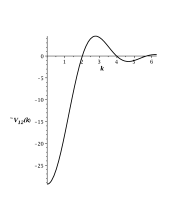
Figure 3: Interaction potential between particles of different kinds in Fourier representation, Eq.(95) for $a=2$. The wave-number $k$ is in $\sigma_{12}^{-1}$ units, the potential is in $v$ units.

$\tilde{V}^{*}_{12}(k)$ is shown in Fig.3 for $a=2$. For this potential the MF instability is given in Eq.(93), in the upper or in the lower line for $k=0$ or for $k_{b}\approx 2.78$ (the first maximum of $\tilde{V}^{*}_{12}(k)$) respectively. In the first case $\tilde{C}^{0}_{12}(0)<0$ and $\tilde{\Phi}_{2}(0)\tilde{\Phi}_{1}(0)>0$, hence the gas-liquid separation occurs. In the second case $\tilde{C}^{0}_{12}(k_{b})>0$ and $\tilde{\Phi}_{2}(k_{b})\tilde{\Phi}_{1}(k_{b})<0$, hence local demixing occurs. In each case $\tilde{C}^{0}_{12}(k_{b})\tilde{\Phi}_{2}(k_{b})\tilde{\Phi}_{1}(-k_{b})<0$ and the Gaussian part of the excess grand potential, Eq.(50), can vanish (in this example $\tilde{C}^{0}_{ii}(k)>0$). The two surfaces in Eq.(93) are shown in Figs.4 and 5 for equal sizes of particles, and in Fig.6 for $\delta=0.95$ ($\sigma_{1}/\sigma_{2}=39$). The period of the most probable inhomogeneities is $2\pi/k_{b}\approx 2.26\sigma_{12}$. For equal sizes $\sigma_{12}=\sigma_{1}$, but in the case of the large size asymmetry the characteristic extent of inhomogeneities is $1.16\sigma_{1}$. This example is at the boundary of applicability of the mesoscopic description.

For equal sizes gas-liquid separation occurs for low volume fractions, and for higher volume fractions the liquid phase undergoes periodic ordering. The MF instability with respect to periodic ordering signals tendency for formation of an “ionic“ crystal, where nearest-neighbors are of different kind [36]. For large size ratio the phase-separation is found for temperatures lower than the temperature at the $\lambda$-surface for all volume fractions. Below the $\lambda$-surface the system is inhomogeneous. Studies beyond MF are necessary to clarify whether transition between gas and lyotropic liquid crystal preempts the gas-liquid separation, or the transition between inhomogeneous fluids (containing clusters or other aggregates) occurs.

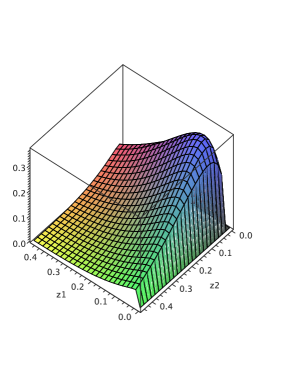
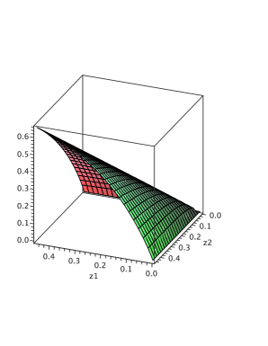
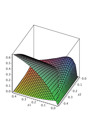
Figure 4: Surfaces representing dimensionless temperature $k_{B}T/v$ at the MF boundary of stability of the homogeneous phase for $\tilde{V}^{*}_{12}(k)$ given in Eq.(94) with $a=2$, and $\tilde{V}_{11}(k)=\tilde{V}_{22}(k)=0$, for equal sizes of particles. Instability with respect to gas-liquid separation is shown in top left panel and instability with respect to periodic ordering ($\lambda$-surface) in top right panel. In bottom panel both surfaces are shown. Volume fractions of the two components (dimensionless) here are denoted by $z1$ and $z2$ and in the text by $\zeta_{1}$, $\zeta_{2}$ respectively.

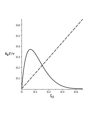
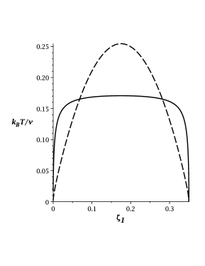
Figure 5: Cross-sections through the surfaces shown in Fig.3 (bottom panel). Left: for equal volume fractions of the two components, $\zeta_{1}=\zeta_{2}$. Right: for $\zeta_{2}=0.35-\zeta_{1}$. Solid and dashed lines represent gas-liquid separation and the $\lambda$-surface (the upper and the lower line in Eq.(93)) respectively. $k_{B}T/v$ and the volume fraction are both dimensionless.

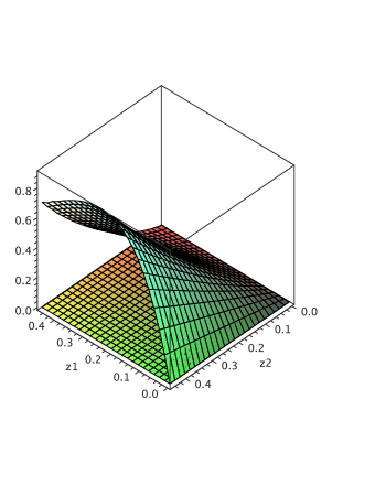
Figure 6: Surfaces representing dimensionless temperature $k_{B}T/v$ at the MF boundary of stability of the homogeneous phase for $\tilde{V}^{*}_{12}(k)$ given in Eq.(94) with $a=2$, and $\tilde{V}_{11}(k)=\tilde{V}_{22}(k)=0$, for $\delta=0.95$ ($\sigma_{1}/\sigma_{2}=39$). The gas-liquid separation (lower surface) is metastable in MF for all values of the volume fractions. Volume fractions of the two components (dimensionless) here are denoted by $z1$ and $z2$ and in the text by $\zeta_{1}$, $\zeta_{2}$ respectively.

Let us summarize the above examples. When the interaction potentials between like particles are attractive for some distances and repulsive for different distances, and the Fourier transform assumes a negative minimum for $k>0$, then the system is inhomogeneous below the $\lambda$-surface. Such behavior was found already in one-component systems. In addition, inhomogeneous structures can occur when particles of different kind attract each other and the Fourier transform of the interaction potential assumes positive maximum for $k>0$. Periodic ordering is enhanced when the size asymmetry increases, and the system becomes inhomogeneous even for low volume fractions for $\delta>0.9$. Increasing tendency for clustering with increasing size asymmetry was observed in ionic systems, in mesoscopic theory [34] and in simulation studies [37, 38].

IV.3 Beyond MF stability analysis

In order to calculate the phase diagram and structure we need to calculate the correlation functions beyond MF. The explicit expressions for the inverse correlation functions in MF in principle allow for obtaining the correlation functions in the Brazovskii-type approximation by self-consistent solutions of Eq.(54). In practice this is less trivial than in the one-component case [32].

The grand potential functional of the mesoscopic volume fractions can be obtained once the matrix $\tilde{\bf C}^{co}(k)$ and its eigenvalues are determined from Eqs.(45)-(49). However, even at the MF level determination of the phase diagram is not quite trivial. The problem simplifies when we restrict our considerations to phases of particular symmetry. In one-component systems the MF phase diagram was determined for weak ordering in Ref.[25, 39], and in two-component case one can proceed in a similar way. The fluctuation contribution to the grand potential can be obtained from Eqs.(45)-(50) and (54). We should stress that from sec.3 it follows that the phase transitions between inhomogeneous phases are first-order. Temperature at the transition is shifted compared to the MF result, because the fluctuation contribution to the grand potential in different phases is different.

V Summary and discussion

We developed a mesoscopic DFT for inhomogeneous mixtures in terms of mesoscopic volume fractions. Local volume fraction is suitable for description of inhomogeneous distribution of particles on mesoscopic length scales when particles of different species are of significantly different sizes. This is because derivation of a Landau-type theory from statistical mechanics requires expansions in local deviations of the volume fraction (or density) from the average value. Since volume fractions are less than unity regardless of the size of the particles, such expansions are justified from mathematical point of view. We performed precise coarse-graining by introducing the microscopic volume fraction, and then by averaging it over mesoscopic regions (see Eq.(8)) to obtain mesoscopic field. This field is next considered as a constraint on the microscopic states. Exact expression for the grand potential consisting of two parts is obtained. The first part contains contributions from the microscopic states that are compatible with the constraint imposed on the volume fractions on the mesoscopic scale - the mesoscopic volume fraction of each component must be equal to the ensemble average. This term has a form similar to the grand potential in standard DFT. The second term is the contribution resulting from mesoscopic fluctuations - that is, from microscopic states that are not compatible with the ensemble average of the volume fraction on the mesoscopic scale. This term in turn has a form similar to the Landau theory.

In practice additional assumptions and approximations are necessary in order to obtain predictions for particular systems in the framework of this theory. Being interested in inhomogeneities on mesoscopic length scale, we assume that ordering occurs on length scales larger than the size of particles, and adopt local density approximation for the hard-sphere reference system. The functional can be further simplified under the assumption of weak ordering, by which we mean that local deviations of the volume fraction from the space averaged value are small. Under the two assumptions, often valid in soft matter, we obtain a functional (Eqs.(45)-(50), (54) and (52)) which is similar to an extension of the Landau theory for mixtures combined with simple DFT. The role of the OP’s is played by linear combinations of the deviations of the local volume fractions from the space-averaged values. Minima of the functional correspond to equilibrium structures. All parameters in the functional are expressed in terms of the free-energy density of hard-spheres and in terms of interaction potentials which can have arbitrary form. In the case of one-component systems we obtain LGW or LB theory, when the interaction potential times the pair distribution function, $V^{co}$, in Fourier representation is approximated by

$$\tilde{V}^{co}(k)=\tilde{V}^{co}(k_{b})+\frac{1}{2}\tilde{V}^{co}(k_{b})^{{}^{\prime\prime}}(k-k_{b})^{2}.$$ (96)

The LGW and LB theories correspond to $k_{b}=0$ and $k_{b}>0$ respectively. In original LB theory the second term in Eq.(96) is proportional to $(k^{2}-k_{b}^{2})^{2}$, but for $k\approx k_{b}$, i.e. for dominant wave-numbers, we have $(k^{2}-k_{b}^{2})^{2}\approx(2k_{b})^{2}(k-k_{b})^{2}$. From the theory developed in Ref.[25] either the LGW or the LB theory is obtained as a further approximation, depending on the form of the interaction potential. We are not aware of extensions of the phenomenological LB theory to mixtures. From the theory developed in this work we can determine whether the system can separate in homogeneous phases, or whether inhomogeneous structures appear on low-temperature side of the $\lambda$-surface. This information can be obtained from the form of interaction potentials and from the size ratio of the particles, by performing stability analysis of the homogeneous phase (secs.3 and 4). In Landau-type theories separation into homogeneous phases or periodic ordering is an apriori assumption.

Despite strong assumptions and approximations, determination of the phase diagram in this theory is not easy, but we can draw some qualitative conclusions already from the relatively simple stability analysis. From the approximate form of the inverse correlation function (Eqs.(54) and (52)) it follows that instability with respect to periodic ordering ($k_{b}>0$) obtained in MF is removed by mesoscopic fluctuations, as was the case also in one component systems. The $\lambda$-surface corresponding to the MF instability may be a borderline between homogeneous and inhomogeneous structure of the disordered phase. For high volume fractions formation of some kind of periodic crystal can be expected on this side of the $\lambda$-surface which corresponds to inhomogeneous structure. For low volume fractions we may expect formation of ordered clusters, where domains with increased and depleted volume fraction of particular components are periodically ordered. However, the clusters (’living polymers’) can have different sizes and locations in space as a result of the mesoscopic fluctuations. Simple examples that illustrate the theory for two components indicate that formation of inhomogeneous distribution of particles is enhanced when the size ratio between the particles of different components increases. Further work is necessary for determination of phase diagrams for particular systems within the framework of the theory developed in this work, and for verification of validity of our approximations in different experimental systems. It is important to note that formation (or not) of inhomogeneous distribution of particles in mixtures depends not only on the interaction potentials, but on a combined effect of interactions and size ratios. In future studies predictions of this theory for two components should be compared with predictions of the theory in which only the big particles are taken into account explicitly, and the small components lead only to solvent-mediated effective interactions.

Acknowledgments This work is dedicated to Prof. Robert Evans on the occasion of his birthday. I would like to thank Dr. Oksana Patsahan for fruitful discussions. Partial supports by the Polish Ministry of Science and Higher Education, Grant No NN 202 006034, and by the Ukrainian-Polish joint research project “Statistical theory of complex systems with electrostatic interactions” are gratefully acknowledged.

VI Appendix

The partial derivatives of the dimensionless free-energy density for hard spheres, $f^{*}_{\alpha\beta}(\zeta_{1},\zeta_{2})=\sigma_{12}^{3}\beta f^{h}_{\alpha\beta}(\zeta_{1},\zeta_{2})$ are obtained from the explicit expressions for the chemical potentials in the hard-sphere mixture derived in Ref.[33]. Direct differentiations lead to the following expressions

$$f^{*}_{\alpha\alpha}(\zeta_{1},\zeta_{2})=\frac{6}{\pi r_{\alpha}^{3}}\Bigg{[}\frac{1}{\zeta_{\alpha}}+\frac{8}{1-\zeta}+\frac{15r_{\alpha}X_{1}+6r_{\alpha}^{2}X_{2}+r_{\alpha}^{3}X_{3}}{(1-\zeta)^{2}}$$ (97)

$$+\frac{18r_{\alpha}^{2}X_{1}^{2}+6r_{\alpha}^{3}X_{1}X_{2}}{(1-\zeta)^{3}}+\frac{9r_{\alpha}^{3}X_{1}^{3}}{(1-\zeta)^{4}}\Bigg{]}$$

and

$$f^{*}_{12}(\zeta_{1},\zeta_{2})=\frac{6}{\pi(r_{1}r_{2})^{3}}\Bigg{[}\frac{8}{1-\zeta}+\frac{2r_{1}r_{2}(6+r_{1}r_{2})X_{1}+8r_{1}^{2}r_{2}^{2}X_{2}}{(1-\zeta)^{2}}$$ (98)

$$+\frac{18r_{1}^{2}r_{2}^{2}X_{1}^{2}+6r_{1}^{3}r_{2}^{3}X_{1}X_{2}}{(1-\zeta)^{3}}+\frac{9r_{1}^{3}r_{2}^{3}X_{1}^{3}}{(1-\zeta)^{4}}\Bigg{]}$$

where

$$X_{n}=\frac{\zeta_{1}}{r_{1}^{n}}+\frac{\zeta_{2}}{r_{2}^{n}}$$ (99)

and $r_{\alpha}$ is defined in Eq.(63)

References

- [1] J. Hansen and I. McDonald, Theory of Simple Liquids (Academic Press, London, 1976).
- [2] Zinn-Justin, Quantum Field Theory and Critical Phenomena (Clarendon Press, Oxford, 1989).
- [3] D.J. Amit, Field Theory, the Renormalization Group and Critical Phenomena (World Scientific, Singapore, 1984).
- [4] I. Yukhnovskii, Sov.Phys. JETP 34, 263 (1958).
- [5] I.R. Yukhnovskii, Phase Transitions of the Second Order, Collective Variable Methods (World Scientific, Singapore, 1978).
- [6] J.M. Caillol, O. Patsahan and I. Mryglod, Physica A 368, 326 (2006).
- [7] A. Parola and L. Reatto, Phys. Rev. A 31, 3309 (1985).
- [8] A. Parola and L. Reatto, Adv. Phys. 44, 211 (1995).
- [9] O. Patsahan, Physica A 272, 358 (1999).
- [10] D. Pini, J. Ge, A. Parola and L. Reatto, Chem. Phys. Lett. 327, 209 (2000).
- [11] A. Stradner, H. Sedgwick, F. Cardinaux, W. Poon, S. Egelhaaf and P. Schurtenberger, Nature 432, 492 (2004).
- [12] A.I. Campbell, V. J.Anderson, J.S. van Duijneveldt and P. Bartlett, Phys. Rev. Lett. 94, 208301 (2005).
- [13] A.J. Archer, D. Pini, R. Evans and L. Reatto, J. Chem. Phys. 126, 014104 (2007).
- [14] A.J. Archer and N.B. Wilding, Phys. Rev. E 76, 031501 (2007), and references therein.
- [15] D. Pini, A. Parola and L. Reatto, J. Phys.:Cond. Mat. 18, S2305 (2006).
- [16] A. Imperio and L. Reatto, J. Phys.:Cond. Mat. 16, 3769 (2004).
- [17] S.A. Brazovskii, Sov. Phys. JETP 41, 8 (1975).
- [18] L. Leibler, Macromolecules 13, 1602 (1980).
- [19] M. Teubner and R. Strey, J. Chem. Phys. 87 (5), 3195–3200 (1987).
- [20] G.H. Fredrickson and E. Helfand, J. Chem. Phys. 87, 67 (1987).
- [21] G. Gompper and M. Schick, Phys. Rev. E 49 (2), 1478–1482 (1994).
- [22] V.E. Podneks and I.W. Hamley, Pis’ma Zh. Exp. Teor. Fiz. 64, 564 (1996).
- [23] A. Ciach and W.T. Góźdź, Annu. Rep.Prog. Chem., Sect.C 97, 269 (2001), and references therein.
- [24] R. Evans, Adv. Phys. 28, 143 (1979).
- [25] A. Ciach, Phys. Rev. E 78, 061505 (2008).
- [26] M. Dijkstra, J.M. Brader and R. Evans, J. Phys.:Cond. Mat. 11, 10079 (1999).
- [27] M. Dijkstra, R. van Roij and R. Evans, J. Chem. Phys. 113, 4799 (2000).
- [28] A. Ciach and O. Patsahan, Phys. Rev. E 74, 021508 (2006).
- [29] A. Ciach and G. Stell, J. Mol. Liq. 87, 255 (2000).
- [30] A. Ciach, W.T. Góźdź and R.Evans, J. Chem. Phys. 118, 3702 (2003).
- [31] A. Ciach, Phys. Rev. E 73, 066110 (2006).
- [32] O. Patsahan and A. Ciach, J. Phys.: Condens. Matter 19, 236203 (2007).
- [33] J.L. Lebowitz and J.S. Rowlinson, J. Chem. Phys. 41, 133 (1964).
- [34] A. Ciach, W.T. Góźdź and G. Stell, Phys. Rev. E 75, 051505 (2007).
- [35] O. Patsahan and T. Patsahan, Phys. Rev. E 81, 031110 (2010).
- [36] A. Ciach, W.T. Góźdź and G. Stell, J. Phys. Cond. Mat. 18, 1629 (2006).
- [37] D. Cheong and A. Panagiotopoulos, J. Chem. Phys. 119, 8526 (2003).
- [38] E. Spohr, B. Hribar and V. Vlachy, J. Phys. Chem B. 106, 2343 (2002).
- [39] A. Ciach and W.T. Góźdź, Condensed Matter Physics 13, 23603 (2010).