Methodological Issues in Multistage Genome-Wide Association Studies

Abstract

Because of the high cost of commercial genotyping chip technologies, many investigations have used a two-stage design for genome-wide association studies, using part of the sample for an initial discovery of “promising” SNPs at a less stringent significance level and the remainder in a joint analysis of just these SNPs using custom genotyping. Typical cost savings of about 50% are possible with this design to obtain comparable levels of overall type I error and power by using about half the sample for stage I and carrying about 0.1% of SNPs forward to the second stage, the optimal design depending primarily upon the ratio of costs per genotype for stages I and II. However, with the rapidly declining costs of the commercial panels, the generally low observed ORs of current studies, and many studies aiming to test multiple hypotheses and multiple endpoints, many investigators are abandoning the two-stage design in favor of simply genotyping all available subjects using a standard high-density panel. Concern is sometimes raised about the absence of a “replication” panel in this approach, as required by some high-profile journals, but it must be appreciated that the two-stage design is not a discovery/replication design but simply a more efficient design for discovery using a joint analysis of the data from both stages. Once a subset of highly-significant associations has been discovered, a truly independent “exact replication” study is needed in a similar population of the same promising SNPs using similar methods. This can then be followed by (1) “generalizability” studies to assess the full scope of replicated associations across different races, different endpoints, different interactions, etc.; (2) fine-mapping or resequencing to try to identify the causal variant; and (3) experimental studies of the biological function of these genes. Multistage sampling designs may be more useful at this stage, say, for selecting subsets of subjects for deep resequencing of regions identified in the GWAS.

, , , ,
and

1 Introduction

Many of the genome-wide association studies(GWAS) currently underway or already reported have used some form of multistage sampling design (Satagopan et al., 2002) because of the considerable savings in genotyping costs this approach offers. In Section 2 we provide an overview of the basic approach to designing such studies, touching on such topics as the trade-offs between sample size and marker density, the selection of markers to carry forward to the second stage, methods of significance testing, the use of DNA pooling, and multistage designs for testing gene–environment (G${}\times{}$E) and gene–gene (G${}\times{}$G) interactions. Section 3 considers the general question of whether two-stage designs are still necessary in an era of declining costs and multipurpose studies. Finally, Section 4 discusses what should be done after a completed GWAS, including replication, fine mapping, generalizability and functional studies, and revisits the utility of multistage designs in this context.

2 Basic Principles of Two-Stage Study Design for GWAS

Two-phase case-control designs were introduced to the epidemiologic literature by White (1982) and have been extensively developed in a series of papers by Breslow and various colleagues (for a general overview of this literature, see Breslow and Chatterjee, 1999). The basic idea of these designs is to use information available on all subjects in the main study to draw a more informative subsample for additional, more expensive, measurements, combining the information from both phases in the analysis.

Two-stage sampling for GWAS, as introduced by Satagopan et al. (2002), is quite different, based on genotyping part of the sample using a commercial high-density panel (typically 300,000 to a million SNPs) and then genotyping the most promising SNPs using a customized panel on the remainder of the sample. A final analysis combining the information from both samples is more powerful than treating the design as a hypothesis generation followed by independent replication (Skol et al., 2006; Yu et al., 2007) because it exploits the additional information about how significant the first stage associations were, not just the fact that they exceeded some threshold. Formally, two stage designs can be conceptualized as a family of group sequential tests (one per SNP) with allowance for early stopping for “futility” (Jennison and Turnbull, 2000).

Optimization of the design is usually framed as choosing the significance levels and the allocation of samples between the two stages in such a manner as to minimize the total cost while attaining the desired genome-wide significance level and power (Kraft, 2006; Kraft and Cox, 2008; Muller, Pahl and Schafer, 2007; Saito and Kamatani, 2002; Satagopan and Elston, 2003; Satagopan, Venkatraman and Begg, 2004; Service, Sandkuijl and Freimer, 2003; Skol et al., 2007; Wang et al., 2006); alternatively, one might wish to maximize power subject to total sample size, genotype cost and type I error, or to minimize the total sample size subject to the other factors. These optimal designs are insensitive to the genetic model (mode of inheritance, relative risk and allele frequencies) and determined primarily by the total number of markers to be genotyped in stage I, the relative cost per genotype at stages I and II, the total available sample size, and whether (and how many) additional flanking markers will be tested around those selected from stage I. As an example of a cost minimization, the optimal design for a cost ratio of about 17.5 with 500K markers being tested in stage I and no additional SNPs being tested at stage II turns out to involve testing 30% of the sample in stage I at a significance level of 0.0037 (i.e., about 1850 markers tested in stage II) and a significance level for the joint analysis of 1.6${}\times 10^{-7}$ (Wang et al., 2006); in this case, about 87% of the total cost goes to stage I genotyping, but the total cost is only 40% that of a comparably powered one-stage design.

Several authors (Eberle et al., 2007; Gail et al., 2008; Nannya et al., 2007) have investigated the power of GWAS, either for a single-stage or the first-stage of a multistage scan, and generally concluded that sample sizes of 1000 cases and 1000 controls were sufficient to detect associations in the range of 1.7–2.0, smaller relative risks (e.g., 1.2–1.3) requiring much larger sample sizes. In general, minimum-cost two-stage designs can require considerably larger sample sizes than single-stage designs to achieve the same power. However, large costs reductions can still be achieved with a “nearly optimal” two-stage design using a sample size only slightly larger than a one-stage design (Wang et al., 2006).

2.1 Trade-off Between Sample Size andMarker Density

A crucial decision to be made is the choice of genotyping platform for stage I. At this writing, two companies—Affymetrix and Illumina—offerplatforms ranging from 300K to 1M SNPs. The panels differ in the way SNPs were selected and, hence, their coverage ($r^{2}$) of the remaining commonHapMap SNPs, as well as in their laboratory performance (call rates, reproducibility, etc.). Because coverage of SNPs is highly variable across the genome and the relationship between power and $r^{2}$ is nonlinear, the average power to detect an association with a random SNP is smaller than the power based on the average $r^{2}$ (Jorgenson and Witte, 2006). Instead, one must average the power for a given noncentrality parameter $\lambda$ at a putative causal locus across the distribution of $r^{2}$s. The consequence is that one cannot simply add additional sample size to cover regions with poor coverage! For single stage studies, average power is maximized by choosing the platform with the best coverage on which it is affordable to genotype all available samples. Comparisons of recent platforms tend to show that when genotyping budget is limiting, sacrificing sample size for the higher density platform is not usually appropriate (Hao, Schadt and Storey, 2008; Lewinger et al., 2007b; Nannya et al., 2007). A two-stage design, however, can alter the sample-size vs. coverage trade-off in favor of higher density platforms in the first stage by allowing the use of all the available samples at a lower cost. Imputation, on the other hand, reduces the differences between SNP panels, making the lower cost, lower density platforms more attractive (Anderson et al., 2008). See also Barrett and Cardon (2006), de Bakker et al. (2005) and Pe’er et al. (2006) for further discussion.

2.2 Design Complications

2.2.1 Additional markers

Additional markersflanking some or all hits might also be added to better characterize the full range of genetic variation in the region (Saito and Kamatani, 2002; Wang et al., 2006). With 5 additional markers being tested for each hit, the optimal design for the situation discussed above raises the first stage sample size to 49% and reduces significance levels to 0.0005 and 0.5${}\times 10^{-7}$ respectively, so that 95% of the total cost goes to stage I genotyping. In these calculations, it was assumed that the additional markers would be imputed for the first-stage sample, using methods described in Section 2.2.2 and more comprehensively elsewhere in this issue (Su et al., 2009), but one could instead test them directly on the stage I samples first and then decide which ones to carry forward to stage II. Further work on optimization of such designs is still needed.

While it seems intuitively appealing to also use the replication step for the purpose of fine mapping—that is, to see whether there is another marker in the region that shows even stronger evidence for association—the yield from doing so may be minimal. Consider the three possible situations: (1) an associated marker is in perfect LD with a causal variant; (2) it is in weak LD with a causal variant; or (3) it is nowhere near the causal variant. Only in the second case would adding additional markers be of any help. Suppose the first stage sample has power $1-\beta_{1}$ to detect the first kind of association and $1-\beta_{2}$ for the second, and let $\pi_{k}$ denote the prior probability of type $k$. Then the prior probability that the association is of type 2 given $p<\alpha_{1}$ is

$$\frac{(1-\beta_{2})\pi_{2}}{(1-\beta_{1})\pi_{1}+(1-\beta_{2})\pi_{2}+\alpha_{1}\pi_{3}}.$$

Considering the coverage of current platforms, $\pi_{1}$ is probably larger than $\pi_{2}$ and $\pi_{3}$ is certainly much larger, so most detected associations are likely to be of types 1 or 3 and additional markers will not help [Peter Kraft, personal communication].

Clarke et al. (2007) have shown theoretically and by simulation that the increased penalty for multiple comparisons can defeat any possible gains in power for replication. Nevertheless, the inclusion of additional markers can be advantageous in regions of relatively high LD when the original signal is weak, such as in regions where the coverage by the original panel is poor, but then any new associations discovered in the “replication” stage would require yet further confirmation. In general, they recommend deferring fine mapping to a separate sample from that used for replication. Thus, fine mapping should be reserved for the regions that are interesting in the combined stage I and stage II data, rather than incorporated into stage II for all markers carried over from stage I. This keeps the multiple comparisons problem at a minimum whether or not a new (third) sample is used for fine mapping.

2.2.2 Haplotypes, multimarker tests and imputation of missing markers

The commercial panels are designed to allow for testing not just the hundreds of thousands or a million SNPs on the panel, but also all the roughly 5M common variants in the human genome they tag, including copy number variants. This entails using some form of multimarker or haplotype-based approach to “impute” genotypes to all those variants that are not directly tested. Promising associations with imputed variants detected in the initial scan are then tested in either the original sample or the follow-up stage by direct genotyping. While at first blush it might seem that the multiple comparisons penalty for testing 5M variants would offset the advantage of using a tag-SNP approach, the correlation between tests due to LD means that the “effective number of independent tests” is only about 1M in European-descent populations or 2M in African-descent populations (Pe’er et al., 2008). Four companion papers in this issue (Chatterjee et al., 2009; Su et al., 2009; Goddard et al., 2009; Zöllner and Teslovich, 2009) address various aspects of this topic in greater detail.

2.2.3 Family-based designs

One compelling advantage of a two-stage approach may be the opportunity to exploit different study designs, in particular, family- and population-based. For example, the Cancer Family Registries for breast and colorectal cancer are currently undertaking GWASs aimed at exploiting their unique resource, combining the two sampling schemes (Zheng et al., 2010). In the first stage, a population-based series of cases that is enriched for a positive family history or young age at onset is compared with unrelated population controls; hits from this stage are then to be tested using family-based association tests (FBAT) in the second stage using sibling or cousin controls to weed out false positives due to population stratification (see the contribution by Astle and Balding, 2009 in this issue), and finally, in a third stage, combining the phenotypes of all relatives from extended pedigrees with all available genotypes in a conditional segregation analysis (Hopper et al., 1999). A different two-stage design uses between-family comparisons to select a subset of SNPs with high power to detect associations in an FBAT, and tests associations with this subset using within-family comparisons in the same data set (Van Steen et al., 2005). For further discussion of these various options, see the companion paper in this issue by Laird and Lange (2009).

If instead of a FBAT design, some form of genomic control is to be used with population-based case-control studies in a two-stage design, then problems can arise if the subjects in the two stages are derived from different populations. One approach is to estimate kinship using the available data from the different stages (a high-density chip for stage I, just the selected SNPs and perhaps some additional ancestry-informative markers in stage II).

2.2.4 More than two stages?

In principle, there is no reason why the two-stage design described above could not be extended to a multistage design, with successively smaller proportions of SNPs being tested in new samples at each subsequent stage. Indeed, some of the earliest studies were conducted in just that manner (Hirschhorn and Daly, 2005). Multiple stages would have the practical effect of reducing the genotyping cost ratio between the first stage and the combined later stages, perhaps by a significant factor. Inclusion of additional stages would be most cost effective when the genotyping cost ratio is 1 between the platforms used in the second and later stages (Kraft et al., 2008). The additional complexities in both design optimization and final significance testing of results have yet to be fully explored, however.

2.3 Methods of Significance Testing for Two-Stage Designs

Two-stage designs pose special challenges to significance testing in the final analysis of the combined data. The basic $p$-value to be computed is the probability that a given SNP would have been deemed “promising” at the first stage and that the combined data would show significance at a genome-wide level given that it was selected for testing in the second stage, under the null hypothesis that it is not associated with disease. The fact that two “hurdles” have to be crossed for each “significant” result means that the $p$-value of interest is actually somewhat smaller than the “nominal” $p$-value based on analyzing the combined data. The various two-stage design papers discussed earlier have shown how to compute this probability under simplifying assumptions and thereby optimize the design, but these approximations can often be improved upon in analyses of real data. Among other assumptions is that of independence across SNPs, which is necessary to derive the appropriate cutoff for genome-wide significance. An obvious way to avoid having to make such assumptions is some form of a permutation test. For a single-stage design, this is straightforward: one could simply hold the genotypes fixed (thereby maintaining their LD structure) and randomly permute the phenotypes in a standard case-control design (or analogous methods for family-based studies, based on within-family permutation). In a two-stage design, this is not so straightforward, however, as one must permute the entire analysis; but a random permutation of the stage-one data would yield a different set of SNPs to be tested in stage II and these genotypes are not available for permuting!

Two methods have been proposed to assess significance in two-stage studies. They both make clever use of the fully genotyped stage I subjects to mimic the effect of having two stages of genotyping. Both require large numbers of subjects in stages I and II, an assumption that would be usually met for a well-powered GWAS. In Dudbridge’s (2006) method, a permutation null distribution is computed by performing the full two-stage analysis on a large number of permuted datasets in which a subsample of the stage I subjects plays the role of the stage I sample, and the original stage I subjects play the role of the combined stage I and stage II samples. The method is valid under exchangeability of the stage I and stage II samples, provided the permutation distribution “stabilizes” for large samples. The Monte Carlo method of Lin (2006) relies on the fact that the efficient scores functions have, jointly for all tests in stages I and II, a mean-zero asymptotic multivariate normal distribution under the complete null hypothesis, and that all score, Wald or likelihood ratio test statistics commonly used to test single SNPs or haplotypes are asymptotically equivalent to simple chi-square statistics based on the efficient score functions. Assuming that the subjects are randomly chosen for stages I and II, the asymptotic variance matrix of the efficient scores can be estimated based on the observed efficient score functions for stage I only. Monte Carlo replicates can then be efficiently drawn from the estimated asymptotic multivariate normal distribution of the efficient scores, and the chi-square statistics equivalent to the original tests computed for each Monte Carlo replicate. Adjusted $p$-values can be computed based on the Monte Carlo replicates. An advantage of Lin’s method is that it does not require recalculation for each Monte Carlo replicate of the original tests statistics that can be computationally costly, but only for the simpler equivalent chi-square tests based on the efficient scores. This can result in significant time savings. Both Lin’s and Dudbridge’s method can be extended to two-stage family-based GWAS but not to studies using case-control samples in stage I and families in stage II.

Methods based on Bonferroni correction using an “effective number of tests” (see Section 2.2.2) for a given platform in a single-stage design have typically relied on permutation tests applied to data sets where very large numbers of SNPs are genotyped in relatively small numbers of subjects (e.g., the HapMap). Just as for the methods described above, there is an implicit assumption in these calculations that the null distribution of the minimum $p$-value for a group of tests does not depend very strongly on the number of subjects in the analysis but only on the LD pattern between the tests considered.

The entire subject of adjustment for multiple comparisons is rapidly evolving. For a recently proposed method and a review of other methods, see Han, Kang and Eskin (2009).

2.4 Selection of SNPs for the Next Stage

Another decision entails the selection of SNPs to be carried from stage I to stage II or to be reported as “significant” at the end of the study. Of course the true causal association may not lie anywhere near the top of the distribution of $p$-values (Zaykin and Zhivotovsky, 2005). Furthermore, if the distribution includes some false positives due to bias (e.g., differential genotyping error), then the most significant findings are more likely to be false positives.

Most of the literature has assumed that $p$-values for single SNP associations will be used for selecting SNPs to carry forward, although alternatives have been suggested, including the population attributable risk (Hunter and Kraft, 2007), the False Positive Report Probability (Hunter and Kraft, 2007; Samani et al., 2007), Bayes factors or $q$-values (Wakefield, 2008), empirical Bayes estimates of effect size (Hunter and Kraft, 2007) or multimarker methods like a local scan statistic (Guedj et al., 2006). But such approaches make no use of any external information that might suggest that some associations were more credible than others a priori. For example, one might wish to give greater credence to associations with SNPs located in or near genes (particularly those that may have a high prior probability of involvement in the disease) or highly conserved regions of the genome, coding SNPs, those located under a linkage peak, or those with previously reported associations. Often such information is used informally at the conclusion of a GWAS in deciding which associations to pursue with further fine mapping or functional studies.

Roeder et al. (2006) and Roeder, Devlin andWasserman (2007) have proposed a weighted False Discovery Rate framework and Bayesian versions have been proposed by Whittemore (2007) and Wakefield (2007). All of these allow a specific variable to be used to up- or down-weight the significance assigned to each association. They showed that well chosen prior information can substantially improve the power for detecting true associations, while there was relatively little loss of power if that information is uninformative.

Each of these approaches allows only a single variable to be incorporated, with weights specified in advance. Hierarchical modeling approaches (Chen and Witte, 2007; Lewinger et al., 2007a) allow multiple sources of information to be empirically weighted in models for the probability that an association is null and the expectation of the magnitude of an association given that it is not null. Simulation studies (Lewinger et al., 2007a) showed that when there was little or no useful prior knowledge, the standard $p$-value ranking performed best, but when at least some of the available covariates were strongly predictive (even if one did not know which ones were truly predictive), the hierarchical Bayes ranking led to better power. For further discussion, see the paper by Pfeiffer, Gail and Pee (2009) in this issue.

2.5 DNA Pooling

DNA pooling offers another approach that could drastically reduce the cost of genotyping for a GWAS. While the idea has been around for some time (Bansal et al., 2002; Risch and Teng, 1998), the technical challenges in forming comparable pools and quantifying allele frequencies are formidable (Barratt et al., 2002; Feng, Prentice and Srivastava, 2004; Pfeiffer et al., 2002; Sham et al., 2002; Zou and Zhao, 2004). It is only recently that it has proved feasible to apply this technique to high-density genotyping arrays (Craig et al., 2005; Docherty et al., 2007; Johnson, 2007; Meaburn et al., 2006; Sebastiani et al., 2008; Zuo, Zou and Zhao, 2006). As currently employed, the design generally entails forming several small pools of cases and of controls in stage I and selecting SNPs on the basis of their differences in allele frequencies. These are then retested by individual genotyping in stage II, possibly on both the original and a second sample. Much remains to be done to study the best choices of design parameters (numbers of pools, sample sizes, criteria for selecting SNPs to test by individual genotyping, etc.) (Macgregor, 2007) and to estimate the statistical power and false discovery rate for this approach in practice. However, empirical applications have demonstrated that DNA pooling is capable of detecting several associations that have previously been discovered and confirmed by individual genotyping in a GWAS context (Pearson et al., 2007). Furthermore, several studies using this approach have reported novel associations (Kirov et al., 2009; Spinola et al., 2007; Steer et al., 2007), although it remains for these associations to be confirmed independently.

Several recent technological advances offer the potential to greatly improve the utility of DNA pooling. The first entails molecular “bar coding” of the individual DNA molecules contributing to each pool (Craig et al., 2008), so that the genotypes of the specific individuals contributing to the subset of pools found to contain rare variants in excess in case pools compared to control pools can be readily reconstructed without the need for further genotyping. The second development entails the use of “pools of pools” to dramatically reduce the cost, so that it now becomes feasible to obtain DNA sequence information on pools as large as 3000 (D. Duggan, TGen, personal communication). We will revisit the use of multistage designs using pooled DNA for deep-resequencing in the concluding section.

2.6 Multistage Designs for Testing Main Effects and Interactions

The NIH “Genes and Environment Initiative” has focused attention on the use of GWAS for identifying genes that modify the effects of environmental agents (Kraft et al., 2007). Such studies pose additional methodological problems, beyond the usual challenges in assessing the main effects of genes and environmental factors, such as low power (Gauderman, 2002) (for further discussion, see the paper by Kooperberg et al., 2009 in this issue). However, there is the opportunity to improve power by using a case-only design (Piegorsch, Weinberg and Taylor, 1994) in which G${}\times{}$E interaction is tested by testing for association between a gene and environmental factor among cases, under the assumption that this association does not exist in the general population. Such an assumption is not likely to hold for all possible SNP${}\times{}$E interactions in a GWAS, but testing this assumption first in controls and deciding whether to perform a case-only or conventional case-control test accordingly can lead to substantial inflation of type I error rates (Albert et al., 2001). Nevertheless, more appropriate methods for combining the inferences from case-control and case-only analyses of the same data have been described (Chatterjee and Carroll, 2005; Chatterjee, Kalaylioglu and Carroll, 2005; Cheng, 2006; Mukherjee et al., 2007; Mukherjee et al., 2008; Mukherjee and Chatterjee, 2008). For example, Mukherjee and Chatterjee (2008) use an empirical Bayes compromise between the case-only and case-control estimators, weighted by the estimated probability of the existence of a G$-$E association. Rather than limiting the analysis to an all-or-nothing choice between case-only and case-control approaches, these methods have the advantage of letting the data and a prior estimate the most appropriate weight between models. In the case of SNP${}\times{}$SNP interactions, one may use LD information from HapMap to generate flexible priors that can greatly increase power (Li and Conti, 2009). In the context of a GWAS, various multistage designs are possible, such as using a case-only test in the combined sample of cases and controls to screen interaction effects and then confirming that subset by a standard case-control test in the same data set (Murcray, Lewinger and Gauderman, 2009). This design has been shown to be substantially more efficient than a single-stage scan using a standard case-control comparison.

3 Single vs. Two-Stage Designs

As the cost of commercial chips falls relative to custom genotyping, the merits of this approach will need to be reconsidered (Hunter et al., 2007). As mentioned above, faced with a choice between density of SNPs and sample size in a single stage study, it is usually preferable to have the largest possible sample size, even if this means not being able to afford a higher density chip. A two-stage design may, however, allow a higher density chip to be used in stage I than would be affordable in a single-stage design, and hence improve power for regions of low LD and overall mean power (Lewinger et al., 2007b). The ability to combine different study designs (e.g., population-based and family-based) may also favor a two-stage design. Other considerations, however, may favor a one-stage design, such as faster study completion and simplified logistics and quality control due to use of a single genotyping platform. Additionally, multiple hypotheses can be tested using these data, say, multiple phenotypes in a cohort design or various subgroup analyses or interaction tests. For example, in addition to scanning for genetic main effects, the Southern California Children’s Health Study (CHS) of the health effects of air pollution aimed to identify genes that interact with two measures of air pollution, exposure to traffic, in utero, and second-hand tobacco smoke, and GSTM1 (previously shown to be involved in several G${}\times{}$E interactions) or to differ between Hispanic and non-Hispanic children, each of these for two phenotypes, asthma and lung function development. SNPs might be selected from the initial scan for follow-up based on any of these criteria. In order to have reasonable power for detecting each of these effects, a custom panel of 12K markers or more would have been required, the cost of which begins to approach that of simply using the same high density panel as in the initial scan, so the decision was made to do a one-stage scan instead. In fact, in the NHLBI-funded STAMPEED consortium of GWAS for cardiovascular, lung and blood disorders of which the CHS is a part (http://public.nhlbi.nih.gov/GeneticsGenomics/ home/stampeed.aspx), most of the 13 participating centers are using a one-stage design. In a one-stage design, replication of SNPs attaining genome-wide levels of significance is still needed, as discussed below. However, the combination of discovery and replication phases should not be regarded as a formal two-stage design, which we define as involving the testing of a large number of hits in a second stage and doing a joint analysis of both. This may involve optimizing the choice of sample sizes and significance levels as discussed earlier, but these two stages combined have the same goal as a 1-stage design, namely, discovery.

4 After GWAS, what Next?

Multistage sampling designs for GWAS should not be thought of as a hypothesis generation followed by independent replication approach but rather as simply a more cost-efficient way of conducting the discovery approach (Skol et al., 2006). Nevertheless, it must be appreciated that any effect estimates (e.g., odd ratios) surviving the entire discovery process will tend to be biased away from the null because attention is focused only on those that are statistically significant, a phenomenon known as the “winner’s curse” (Kraft, 2008; Yu et al., 2007; Zhong and Prentice, 2008; Zollner and Pritchard, 2007). Thus, some form of truly independent replication is needed, both to confirm the existence of the reported associations and to estimate the magnitude of their effect. In the following sections we distinguish between what we will call “exact replication” and “generalization,” the latter being aimed at determining the full extent of a replicated association across populations, phenotypes, modifiers, etc. In addition, an association initially reported may not be with the causal variant itself, but rather with some other variant it is in LD with, so further studies aimed at fine mapping or resequencing the region to identify the culprit may be needed. Finally, once plausible candidates for the causal variants have been identified, there is a need for further experimental studies to understand their biological function and additional in silico and epidemiologic analyses to build a comprehensive model for the causal pathway.

4.1 Replication

Failure to replicate has been a recurring problem with candidate gene association studies, hence a major concern about the new generation of GWASs (Chanock et al., 2007; Ioannidis, 2007). (The companion paper by Kraft, Zeggini and Ioannidis, 2009 in this issue explores the replication issues in greater depth.) True scientific replication must involve something more than a repetition of the study on a second random sampling from the same population using the same methods (Chanock et al., 2007; Clarke et al., 2007), since simply splitting a sample in half and requiring significance at level $\alpha$ in both halves is less powerful than a single analysis of the entire sample at significance level $\alpha^{2}$ (Skol et al., 2006; Thomas et al., 1985). Nevertheless, the goal at this stage should be to avoid failure to replicate because of true differences in effect between the original and follow-up populations, investigation of real heterogeneity being the subject of the next stage (“generalization”). Many granting agencies now expect investigators to discuss plans for follow-up investigations of any associations detected and some high profile journals are requiring replication studies as part of a single report of a genetic association (Anonymous, 1999; Rebbeck et al., 2004). In many cases, this might best be accomplished by collaborations with other groups with data on a genetically similar set of subjects. Failure to replicate may often be due to the use of replication data sets that were not well designed for this purpose because of heterogeneity between the original and replicate data sets or problematic study designs that were generated for different purposes originally. Replication and generalizability are often muddled together even though they are two different questions that are best addressed with different types of study populations—one selected to minimize heterogeneity and the others selected to maximize it.

One question that frequently arises is whether to restrict replication claims to the same marker detected in the initial GWA scan (“exact” replication) or to test additional markers in the region and allow association with any of them (appropriately adjusted for multiple comparisons) to be treated as evidence of replication (“local” replication) (Clarke et al., 2007). In a similar vein, associations first discovered in a GWAS by imputed SNPs should be confirmed by direct genotyping, either in the original samples, or better in independent replication samples, before a genuine association is claimed. In any event, a clear definition of replication is needed: generally this is taken to be a statistically significant association in the same direction, but now not requiring genome-wide multiple testing correction since only a subset of the top-ranking associations will be subject to replication and the magnitude of the original relative risk is likely to have been overestimated.

4.2 Generalization

Once an association has been replicated, it becomes important to investigate the full range of its effects. For example, one of the first questions to address is whether the effect differs across races. If so, this could be a sign that the association is not causal, but only a reflection of a causal effect of some other variant with which it is in LD, the patterns of LD differing across races, and would suggest that further fine mapping of the region is warranted. Furthermore, if there is heterogeneity by race/ethnicity, fine mapping within a race that exhibits the association of interest but has shorter LD blocks would help localize the signal more efficiently than in a race with longer LD blocks. Alternatively, heterogeneity by race could be a reflection of differences across races in the prevalence of some modifying factors—G${}\times{}$E or G${}\times{}$G interactions—indicating that further investigation of effect modification is warranted. Beyond the question of heterogeneity by race/ethnicity, there are other questions of generalizability worth considering. Does the variant have similar effects across different subtypes of the same disease (for example, for colorectal cancer, by location in the colon, age of onset, family history of colorectal or other cancers, presence or absence of selected molecular markers such as microsatellite instability, BRAF mutation, MLH1 methylation)? Does the variant have effects on other phenotypes—intermediate endpoints like incidence or recurrence of polyps for colorectal cancer or other cancer sites or even other diseases with which it might share a common etiologic pathway? After a result is confirmed in a properly designed replication study, we would advocate a strategic approach to the question of generalizability, guided by a careful consideration of the most important knowledge gaps about the disease, rather than the sometimes uncritical exercise of quickly testing for the reported SNP in whatever data sets are readily available (ignoring whether the result would fill an important gap in our knowledge base).

4.3 Fine-Mapping and Deep Resequencing

Unless there is compelling evidence that a newly discovered association with a particular SNP is indeed causal, further fine mapping of the surrounding region is generally appropriate, given that the SNPs on the discovery panel represent at most 20% of all common variants and were selected primarily for their effectiveness at tagging other variants rather than as biologically plausible candidates themselves. Furthermore, it is becoming increasingly evident that multiple rare variants may play an important role in many diseases (Fearnhead et al., 2004; Iyengar and Elston, 2007; Kryukov, Pennacchio and Sunyaev, 2007; Li and Leal, 2008; Pritchard, 2001). This search for the true culprit(s)—which could occur before, after or concurrent with the generalization activities described above—might involve some combination of fine mapping with additional SNPs and deep resequencing and poses interesting challenges for study design, particularly in terms of the balance between additional efforts to fine-map a signal with additional genotyping of previously known variants versus jumping directly to deep resequencing for discovery.

Fine mapping might explore a relatively large region surrounding the associated SNP(s) and be informed by knowledge from HapMap of the LD structure of the region. The goal would be to genotype a denser set of tag SNPs than was possible in the initial GWAS in order to conduct haplotype or multi-marker association tests, as discussed elsewhere in this issue (Su et al., 2009; Goddard et al., 2009; Zöllner and Teslovich, 2009). (For this purpose, one might wish to use a different population, such as those of African descent where LD blocks would tend to be shorter.) Deep resequencing would entail selection of a subset of participants from the main study for complete sequencing of the region to search for other relatively common variants ($\sim$1–5%) that may not have been characterized by HapMap. These variants would then be genotyped in the entire study sample to test for association. Because of the high cost of sequencing, it might be advisable to do the fine mapping first to narrow down the region of interest, but with the advent of next generation sequencing, DNA “bar coding” and DNA pooling methods (Craig et al., 2008), costs are coming down so rapidly that one might want to proceed directly to sequencing. Either approach might benefit from a formal two-stage sampling design, although the cost savings are likely to be more substantial for deep resequencing studies.

4.3.1 Two-stage designs revisited

The basic idea here would be to select a subset of subjects for additional genotyping and/or sequencing who would be most likely to carry a causal variant. This subset of subjects serves two general goals. The first may simply be to characterize the genetic variation or to discover previously unknown variants within the region to then genotype in the larger main study with a more cost-effective genotyping technology. A second goal may be to formally combine the more detailed information for the subgroup with the data from the main study on only the selected SNPs. As mentioned at the outset, this idea has been extensively developed in the literature on “two-phase sampling” in survey design and more recently in epidemiologic applications. Unlike the two-stage designs for GWAS described above, these designs typically entail using information that is readily available on the entire case-control study to select a stratified subsample. For the first goal of characterization only, a sample of only cases may be most efficient (see below). However, if one wishes to sample the subset for more detailed measurements and then combine the two data sets in a joint analysis, one may need to sample both cases and controls. Here, one needs to consider both the optimization of the informativeness of the subset for discovery as well as informativeness for the ultimate case-control analysis that takes the sampling fractions into account. In the present context, the relevant stratifying variables might include case/control status and the SNP genotypes (and possibly exposure variables if detected through a G${}\times{}$E interaction effect). Such an approach has been explored for candidate gene association studies (Thomas, Xie and Gebregziabher, 2004), where information on a dense panel of SNPs in a targeted subsample is combined with a sparser panel from the main study for the purpose of localizing the signal by LD mapping or for testing haplotype associations. Here, each region identified in a GWAS would likely target a different subsample of subjects, based on the available SNPs in that region.

A typical study might involve sequencing a sample of about 48 or 96 individuals over perhaps a 100 Kb region. Assuming that the region size has already been established based on the pattern of SNP or haplotype associations from the initial GWAS, knowledge of the LD structure of the region and possibly additional fine-mapping, how then should this relatively small sample be selected to maximize the chances of discovering the real causal variant(s)?

Suppose first that a positive association has been found with a single SNP (Table 1, top). If not itself causal, this could theoretically reflect either a deleterious effect of another variant in positive LD with it or a protective effect of a variant in negative LD. Of the two possibilities, the former is much more likely, as negative LD with a protective minor allele is unlikely to generate a large positive association at a marker locus (see the second block in Table 1, where a perfectly protective allele in perfect negative LD yields a marker RR of only 1.067). The subjects with the highest yield of causal variants would then be cases carrying the minor allele of the associated SNP, with carrier controls somewhat lower but still much higher than either cases or controls carrying the major allele.

Table 1: Illustrative calculation of probability of carrying a rare causal variant $G$ among cases and controls carrying the major or minor allele at a marker locus $M$ in LD with it: $\operatorname{Pr}(M)=0.2$, $\operatorname{Pr}(G)=0.05$. Bolded entries indicate the highest yield strata in each situation

Marker	Disease	Causal allele		$\bolds{\operatorname{Pr}(G=1|M,Y)}$
$\bolds{M}$	$\bolds{Y}$	$\bolds{G=0}$	$\bolds{G=1}$
Positive marker association
Positive LD and positive causal association
$\delta=0.036,\mathit{RR}_{YG}=2,\mathit{RR}_{YM}=1.22$
$m$	Controls	0.796	0.004	0.005
	Cases	0.758	0.008	0.010
$M$	Controls	0.154	0.046	0.230
	Cases	0.147	0.088	0.374
Negative LD and negative causal association
$\delta=-0.010,\mathit{RR}_{YG}=0,\mathit{RR}_{YM}=1.067$
$m$	Controls	0.750	0.050	0.063
	Cases	0.789	0.000	0.000
$M$	Controls	0.200	0.000	0.000
	Cases	0.211	0.000	0.000
Negative marker association
Negative LD and positive causal association
$\delta=-0.010,\mathit{RR}_{YG}=3,\mathit{RR}_{YM}=0.889$
$m$	Controls	0.750	0.050	0.063
	Cases	0.682	0.136	0.136
$M$	Controls	0.200	0.000	0.000
	Cases	0.186	0.000	0.000
Positive LD and negative causal association
$\delta=0.036,\mathit{RR}_{YG}=0.5,\mathit{RR}_{YM}=0.887$
$m$	Controls	0.796	0.004	0.005
	Cases	0.816	0.002	0.003
$M$	Controls	0.200	0.046	0.230
	Cases	0.211	0.024	0.130

Now suppose instead that the minor allele shows a negative association with disease. Again, if not itself causal, this could reflect either a protective effect of a variant in positive LD with it or a deleterious effect of a variant in negative LD, these two scenarios now being roughly equally plausible (see bottom two blocks of Table 1, where both configurations yield similar marker RRs). In this case, the most informative subjects would be cases carrying the major allele or controls carrying the minor allele at the associated SNP, with the latter generally having a higher yield of causal variants.

To summarize the situation with a single marker, if one is purely interested in maximizing the chances of identifying a causal variant that will then be genotyped in the entire sample, then one could sample only carriers of the minor allele—cases if the marker association is positive, controls if it is negative. No weighting would be required for the analysis of the full study data for the discovered genotypes. If, on the other hand, one wishes to perform a joint analysis of the main and substudy data incorporating the full sequence data on substudy subjects, then to be able to weight the analysis correctly, all four strata must be represented. The optimal sampling fractions would depend upon knowledge of the true LD and causal association parameters, but one could be guided by the general calculations illustrated in Table 1: if the association with the minor allele is positive, then sample the largest number of cases with the minor allele, then controls with the minor allele, and the smallest number of carriers of the major allele; if the association is negative, then sample most heavily controls with the minor allele, then equal numbers of cases with the minor allele and controls with the major allele, and the smallest number of controls with the minor allele.

Now, suppose the association is not just with a single SNP in a region but with several. A sensible sampling design might now entail first constructing a risk index, say, by logistic regression of case-control status on multiple SNPs or haplotypes and then stratifying jointly on this genetic risk index and case-control status. The concept of positive or negative association and LD is now moot and needs to be replaced by consideration of the shape of the distribution of the risk index (Figure 1). Typically, one might find a relatively small proportion of subjects with a broad range of high risk scores and a large proportion with generally low risk (Thomas et al., 2008). In this situation, it would be cases with high risk scores that are likely to be the most informative, although controls with high risk scores would also have an increased probability of carrying a causal allele. In the event that the risk distribution has a long tail of low risk, it could be worthwhile to sample controls with low risk scores, but detecting effects of rare beneficial alleles would require enormous sample sizes. (Of course, a beneficial effect of a common allele is equivalent to a deleterious effect of a rare allele.) As in the single-marker case, if the purpose is simply to discover potentially causal variants, then one could restrict the sample to high-risk cases, but if a joint analysis is planned, then a well-defined sampling scheme is required that assigns nonzero sampling probability to every individual. This could be accomplished by stratifying jointly on $Y$ and $\operatorname{Pr}(Y=1|\mathbf{M}$) or in proportion to an estimated $\operatorname{Pr}(G=1|Y,\mathbf{M}$) for some hypothesized model.

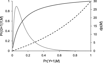
Figure 1: Illustration of a hypothetical distribution of an empirical risk index ($M$, right axis, dotted line) and yield of causal variant carriers ($D=1$, left axis, solid and dashed lines for cases and controls respectively) as a function of $M$.

It must be appreciated that only very strong associations would have any power for testing associations in the subsample alone. The real purpose is simply to identify novel variants that would then be genotyped in the main study. Having completed the sequencing of this stratified sample and genotyping of selected novel variants in the main study, a joint analysis could be performed as described by Thomas, Xie and Gebregziabher (2004) to test for associations with all variants discovered in the resequencing sample, not just those actually genotyped in the main study. This essentially involves imputation of the missing data on main study subjects using the substudy data, but requires appropriate adjustment for the sampling fractions if they depend jointly on genotypes and disease, so that all cells of the stratification must be represented in the sample. For substudy subjects, the standard logistic model can be used by adding as an offset term the log of the ratio of genotype-specific case/control sampling probabilities. For main study subjects, the likelihood contribution becomes a more complex mixture of weighted logistic probabilities, although well approximated by a logistic function if the disease is rare. Of course, imputation of very rare variants in the main study by leveraging a substudy with only a few occurrences of such variants is of dubious value, so all potentially causal variants should be genotyped in the full sample, but imputation could be useful for exploiting LD patterns in the sequence data that might suggest regions worth closer study.

These considerations are likely to be fundamentally altered in the near future by the public availability of resequencing data from the “1000 Genomes Project” (http://www.1000genomes.org/), aimed at identifying variants at a frequency of 1% across the genome in approximately 1500 subjects (500Bantu-speaking, 500 Asian, 500 Caucasian). Data at an intermediate level of detail (e.g., deep resequencing of 1000 genes in 1000 individuals) will be released soon. Once completed, the 1000 Genomes Project will potentially reduce the need for extensive deep resequencing for variants in the 1$-5\%$ range, at least for studies conducted in comparable populations, but would still leave open the question of rarer variants. Methods to leverage the 1000 Genomes data for imputation purposes or joint analysis with a two-phase sampling design, allowing for possible misspecification of the G–M relationships for the specific study’s target population, would be useful.

The advent of whole genome sequence using next-generation sequencing platforms (Mardis, 2008) may also resurrect interest in multistage designs, as genome-wide scans for rare variants are unlikely to be feasible on the tens of thousands of subjects that will be needed, at least until the $1000 genome becomes a reality. Whether this will ever be feasible, given the much larger multiple-testing burden, the sparseness of data on any particular variant and the likelihood that rare variants will be less effectively tagged than common variants, remains to be seen. Nevertheless, these technologies will undoubtedly aid in following up larger and larger regions surrounding SNPs identified in a GWAS on larger and larger samples, requiring adjustment for a much larger universe of variants, rare and common (Hoggart et al., 2008a, 2008b).

4.4 Investigating Biological Function, eQTLs and Pathways

Once a set of highly significant and replicated SNP associations has been found, what then? The challenges posed by the study of the often broadly diverse biologic functions of hits arising from GWASs should not be underestimated. Trying to determine the functionality of even a single GWAS hit can be a daunting task. While clearly in vitro and in vivo experimental studies would be appropriate to investigate function, the initial steps in characterization depend upon whether hits are located within genes, near known genes or in “gene deserts.” If the hit is within a gene, various software packages and web sites could be used to assess the potential functional role of the variant, and such in silico findings could then be confirmed in vitro by molecular approaches such as quantitative RT-PCR. If the hit is near a gene, it could implicate an adjacent gene, but it could also lie in an unannotated gene, an miRNA, or an enhancer or repressor element for some gene located far away (the most likely explanation if it is in a gene desert). Unannotated genes might be identified through tiling gene expression arrays, while in silico and ChIP-chip methods might be used to identify enhancer/repressor elements.

Other types of analyses also might be undertaken that would involve more sophisticated analyses of the GWAS data, either (1) in an attempt to infer causal pathways from the pattern of associations and interactions using the kinds of network analysis tools that have been applied to gene expression and protein interaction data, or (2) to inform the search for effects in the GWAS data by incorporating external knowledge from pathway or genomic databases, literature mining or analysis of gene expression, proteomic, metabolomic or other—omics data, perhaps using hierarchical modeling or gene set enrichment analysis methods. See Chasman (2008), Gieger et al. (2008), Pan (2005) and Wang, Li and Bucan (2007) for discussion of some of these approaches.

A second phase of these studies could be to examine any known biological functionality of the gene in question, and once again those applied approaches will depend upon several considerations such as the likely consequence of the SNP itself upon gene function as well as prior knowledge of the gene and understanding of its involvement, if known, in cellular pathway(s). Gene expression data (even genome-wide data) might be leveraged to identify candidate genes/pathways. A SNP that lies within the coding region of a gene may be more likely to affect the normal function of that gene, either through enhancing its effect or reducing its functionality. Biochemical assays may be available that could be applied to test the effect of a coding region variant on its known gene function, such as a role in apoptosis. Alternatively, where a hit lies adjacent to a gene or within a gene desert and possibly in an enhancer element or other regulatory region, the likely effect may be on the expression level of the gene—whether leading to higher or lower gene expression levels, mRNA stability or post-translational protein levels in target tissues. The next steps of characterization would require using knowledge of that gene and related pathways to develop assays that would test the putative consequences of either elevated or reduced expression of the gene product in appropriate cells. For some genes, accumulated knowledge of its role in the cell may be extensive; however, for others that knowledge may be sparse or even non-existent. Such prior knowledge may be used to help prioritize functional biological studies. However, they could have the effect of steering us away from further characterization of potentially interesting genes that have little prior biological knowledge due to the greater challenges that they pose.

Given the potential complexity and diversity of methods that will need to be applied to follow up on any identified hit, a prioritization scheme will need to be developed that will likely involve many different considerations, such as the strength of the hit itself, whether the hit has any implications for disease subsets such as more aggressive forms of cancer, whether the hit is potentially implicated in more than one disease (such as appears to be the case for the 8q24 region, which is related to at least 4 cancers, and for several diabetes risk alleles that are found to be protective for prostate cancer) and prior biological knowledge. The hierarchical modeling approaches discussed in Section 2.4 may be helpful for combining the evidence from the data at hand and these external sources of knowledge to prioritize hits for follow-up functional studies. None of these kinds of studies would be likely to involve the original epidemiological study subjects, however, and further detailed investigations are likely to be gene-specific, so are beyond the scope of this article.

Two-phase sampling designs may be particularly helpful for biomarker or expression measurements to inform the analysis of pathways. Such analyses may take the form of a network of latent variables, for which the biomarkers are viewed as surrogate measurements (Thomas, 2007). In such designs, one might wish to subsample jointly on some combination of disease, exposure and genotype(s) to select individuals for biomarker measurements. For example, in a pharmacogenetic study, one might subsample on the basis of outcomes and treatment assignment to target a GWAS or a resequencing study of a candidate region; or if GWAS data were already available, one might stratify by a multi-marker risk score, treatment and outcomes for a collection of biomarkers to investigate pathways (Thomas and Conti, 2007). Any study of biomarkers collected after the outcome must, however, address the problem of “reverse causation,” whereby the variable being measured (or the accuracy of its measurement) is affected by the disease or its treatment rather than the other way around.

Finally, it is worth noting that an enhancement in our knowledge of the etiology of disease may have implications that transcend the merely predictive power of a specific variant. The relatively modest relative risks that have been discovered by GWASs for disease etiology could be due in part to selection against high risk variants, but this is unlikely for response to modern pharmacologic agents. For example, SNPs in HMGCR have only a small effect on low density lipoprotein levels, but drugs targeting the protein encoded by HMGCR have a much larger effect (Altshuler, Daly and Lander, 2008). One can at least hope that solving the mystery of how variants in a gene desert such as 8q24 appear to influence the risk of a multitude of cancers would lead to methods aimed at preventing or treating the resulting diseases. Ultimately, the discovery of genetic modifiers of treatment response is central to the goal of personalized medicine.

References

- (1) Albert, P. S., Ratnasinghe, D., Tangrea, J. and Wacholder, S. (2001). Limitations of the case-only design for identifying gene–environment interactions. Am. J. Epidemiol. 154 687–693.
- (2) Altshuler, D., Daly, M. J. and Lander, E. S. (2008). Genetic mapping in human disease. Science 322 881–888.
- (3) Anderson, C. A., Pettersson, F. H., Barrett, J. C., Zhuang, J. J., Ragoussis, J., Cardon, L. R. et al. (2008). Evaluating the effects of imputation on the power, coverage, and cost efficiency of genome-wide SNP platforms. Am. J. Hum. Genet. 83 112–119.
- (4) Anonymous (1999). Freely associating. Nat. Genet. 22 1–2. \MR1715146
- Balding (2009) Astle, W. and Balding, D. J. (2009). Population structure and cryptic relatedness in genetic association studies. Statist. Sci. 24 451–471.
- (6) Bansal, A., van den Boom, D., Kammerer, S., Honisch, C., Adam, G., Cantor, C. R. et al. (2002). Association testing by DNA pooling: An effective initial screen. Proc. Natl. Acad. Sci. USA 99 16871–16874.
- (7) Barratt, B. J., Payne, F., Rance, H. E., Nutland, S., Todd, J. A. and Clayton, D. G. (2002). Identification of the sources of error in allele frequency estimations from pooled DNA indicates an optimal experimental design. Ann. Hum. Genet. 66 393–405.
- (8) Barrett, J. C. and Cardon, L. R. (2006). Evaluating coverage of genome-wide association studies. Nat. Genet. 38 659–662.
- (9) Breslow, N. E. and Chatterjee, N. (1999). Design and analysis of two-phase studies with binary outcome applied to Wilms tumor prognosis. J. Roy. Stat. Soc. Ser. C 48 457–468.
- (10) Chanock, S. J., Manolio, T., Boehnke, M., Boerwinkle, E., Hunter, D. J., Thomas, G. et al. (2007). Replicating genotype-phenotype associations. Nature 447 655–660.
- (11) Chasman, D. I. (2008). On the utility of gene set methods in genomewide association studies of quantitative traits. Genet. Epidemiol. 32 658–668.
- (12) Chatterjee, N., Chen, Y.-H., Luo, S. and Carroll, R. J. (2009). Analysis of case-control association studies: SNPs, imputation and haplotypes. Statist. Sci. 24 489–502.
- (13) Chatterjee, N. and Carroll, R. J. (2005). Semiparametric maximum likelihood estimation exploiting gene–environment independence in case-control studies. Biometrika 92 399–418. \MR2201367
- (14) Chatterjee, N., Kalaylioglu, Z. and Carroll, R. J. (2005). Exploiting gene–environment independence in family-based case-control studies: Increased power for detecting associations, interactions and joint effects. Genet. Epidemiol. 28 138–156.
- (15) Chen, G. K. and Witte, J. S. (2007). Enriching the analysis of genomewide association studies with hierarchical modeling. Am. J. Hum. Genet. 81 397–404.
- (16) Cheng, K. F. (2006). A maximum likelihood method for studying gene–environment interactions under conditional independence of genotype and exposure. Stat. Med. 25 3093–3109. \MR2247229
- (17) Clarke, G. M., Carter, K. W., Palmer, L. J., Morris, A. P. and Cardon, L. R. (2007). Fine mapping versus replication in whole-genome association studies. Am. J. Hum. Genet. 81 995–1005.
- (18) Craig, D. W., Huentelman, M. J., Hu-Lince, D., Zismann, V. L., Kruer, M. C., Lee, A. M. et al. (2005). Identification of disease causing loci using an array-based genotyping approach on pooled DNA. BMC Genomics 6 138.
- (19) Craig, D. W., Pearson, J. V., Szelinger, S., Sekar, A., Redman, M., Corneveaux, J. J. et al. (2008). Identification of genetic variants using bar-coded multiplexed sequencing. Nat. Methods 5 887–893.
- (20) de Bakker, P. I., Yelensky, R., Pe’er, I., Gabriel, S. B., Daly, M. J. and Altshuler, D. (2005). Efficiency and power in genetic association studies. Nat. Genet. 37 1217–1223.
- (21) Docherty, S. J., Butcher, L. M., Schalkwyk, L. C. and Plomin, R. (2007). Applicability of DNA pools on 500 K SNP microarrays for cost-effective initial screens in genomewide association studies. BMC Genomics 8 214.
- (22) Dudbridge, F. (2006). A note on permutation tests in multistage association scans. Am. J. Hum. Genet. 78 1094–1095.
- (23) Eberle, M. A., Ng, P. C., Kuhn, K., Zhou, L., Peiffer, D. A., Galver, L. et al. (2007). Power to detect risk alleles using genome-wide tag SNP panels. PLoS Genet. 3 1827–1837.
- (24) Fearnhead, N. S., Wilding, J. L., Winney, B., Tonks, S., Bartlett, S., Bicknell, D. C. et al. (2004). Multiple rare variants in different genes account for multifactorial inherited susceptibility to colorectal adenomas. Proc. Natl. Acad. Sci. USA 101 15992–15997.
- (25) Feng, Z., Prentice, R. and Srivastava, S. (2004). Research issues and strategies for genomic and proteomic biomarker discovery and validation: A statistical perspective. Pharmacogenomics 5 709–719.
- (26) Gail, M. H., Pfeiffer, R. M., Wheeler, W. and Pee, D. (2008). Probability of detecting disease-associated single nucleotide polymorphisms in case-control genome-wide association studies. Biostatistics 9 201–215.
- (27) Gauderman, W. J. (2002). Sample size requirements for matched case-control studies of gene–environment interaction. Stat. Med. 21 35–50.
- (28) Gieger, C., Geistlinger, L., Altmaier, E., Hrabe de Angelis, M., Kronenberg, F., Meitinger, T. et al. (2008). Genetics meets metabolomics: A genome-wide association study of metabolite profiles in human serum. PLoS Genet. 4 e1000282.
- (29) Goddard, M. E., Wray, N. R., Verbyla, K. and Visscher, P. M. (2009). Estimating effects and making predictions from genome-wide marker data. Statist. Sci. 24 517–529.
- (30) Guedj, M., Robelin, D., Hoebeke, M., Lamarine, M., Wojcik, J. and Nuel, G. (2006). Detecting local high-scoring segments: A first-stage approach for genome-wide association studies. Stat. Appl. Genet. Mol. Biol. 5 Art. 22. \MR2306485
- (31) Han, B., Kang, H. M. and Eskin, E. (2009). Rapid and accurate multiple testing correction and power estimation for millions of correlated markers. PLoS Genet. 5 e1000456.
- (32) Hao, K., Schadt, E. E. and Storey, J. D. (2008). Calibrating the performance of SNP arrays for whole-genome association studies. PLoS Genet. 4 e1000109.
- (33) Hirschhorn, J. N. and Daly, M. J. (2005). Genome-wide association studies for common disease and complex traits. Nat. Rev. Genet. 6 95–108.
- (34) Hoggart, C. J., Clark, T. G., de Iorio, M., Whittaker, J. C. and Balding, D. J. (2008a). Genome-wide significance for dense SNP and resequencing data. Genet. Epidemiol. 32 179–185.
- (35) Hoggart, C. J., Whittaker, J. C., de Iorio, M. and Balding, D. J. (2008b). Simultaneous analysis of all SNPs in genome-wide and re-sequencing association studies. PLoS Genet. 4 e1000130.
- (36) Hopper, J. L., Southey, M. C., Dite, G. S., Jolley, D. J., Giles, G. G., McCredie, M. R. E. et al. (1999). Population-based estimate of the average age-specific cumulative risk of breast cancer for a defined set of protein-truncating mucations in BRCA1 and BRCA2. Cancer Epidemiol. Biomark. Prev. 8 741–747.
- (37) Hunter, D. J. and Kraft, P. (2007). Drinking from the fire hose—statistical issues in genomewide association studies. N. Engl. J. Med. 357 436–439.
- (38) Hunter, D. J., Thomas, G., Hoover, R. N. and Chanock, S. J. (2007). Scanning the horizon: What is the future of genome-wide association studies in accelerating discoveries in cancer etiology and prevention? Cancer Causes Control. 18 479–484.
- (39) Ioannidis, J. P. (2007). Non-replication and inconsistency in the genome-wide association setting. Hum. Hered. 64 203–213.
- (40) Iyengar, S. K. and Elston, R. C. (2007). The genetic basis of complex traits: Rare variants or “common gene, common disease”? Methods Mol. Biol. 376 71–84.
- (41) Jennison, C. and Turnbull, B. W. (2000). Group Sequential Methods with Applications to Clinical Trials xviii. Chapman & Hall/CRC, Boca Raton, FL. \MR1710781
- (42) Johnson, T. (2007). Bayesian method for gene detection and mapping, using a case and control design and DNA pooling. Biostatistics 8 546–565.
- (43) Jorgenson, E. and Witte, J. S. (2006). Coverage and power in genomewide association studies. Am. J. Hum. Genet. 78 884–888.
- (44) Kirov, G., Zaharieva, I., Georgieva, L., Moskvina, V., Nikolov, I., Cichon, S. et al. (2009). A genome-wide association study in 574 schizophrenia trios using DNA pooling. Mol. Psychiatry 14 796–803.
- (45) Kooperberg, C., LeBlanc, M., Dai, J. Y. and Rajapakse, I. (2009). Structures and assumptions: Strategies to harness gene gene and gene environment interactions in GWAS. Statist. Sci. 24 472–488.
- (46) Kraft, P. (2006). Efficient two-stage genome-wide association designs based on false positive report probabilities. Pac. Symp. Biocomputing 11 523–534.
- (47) Kraft, P. (2008). Curses—winner’s and otherwise—in genetic epidemiology. Epidemiology 19 649–651; discussion 657–648.
- (48) Kraft, P. and Cox, D. G. (2008). Study designs for genome-wide association studies. Adv. Genet. 60 465–504.
- (49) Kraft, P., Chanock, C., Hunter, D., Chatterjee, N., and Thomas, G. (2008). Cost-efficient multi-stage designs for genome-wide association studies. In Genetic Dissection of Complex Traits, 2nd ed. (D. C. Rao and C. C. Gu, eds.) 465–504. Academic Press, Boston.
- (50) Kraft, P., Yen, Y. C., Stram, D. O., Morrison, J. andGauderman, W. J. (2007). Exploiting gene–environment interaction to detect genetic associations. Hum. Hered. 63 111–119.
- (51) Kraft, P., Zeggini, E. and Ioannidis, J. P. A. (2009). Replication in genome-wide association studies. Statist. Sci. 24 561–573.
- (52) Kryukov, G. V., Pennacchio, L. A. and Sunyaev, S. R. (2007). Most rare missense alleles are deleterious in humans: Implications for complex disease and association studies. Am. J. Hum. Genet. 80 727–739.
- (53) Laird, N. M. and Lange, C. (2009). The role of family-based designs in genome-wide association studies. Statist. Sci. 24 388–397.
- (54) Lewinger, J. P., Conti, D. V., Baurley, J. W., Triche, T. J. and Thomas, D. C. (2007a). Hierarchical Bayes prioritization of marker associations from a genome-wide association scan for further investigation. Genet. Epidemiol. 31 871–882.
- (55) Lewinger, J. P., Duggan, D. J., Taverna, D. M.,Gauderman, W. J., Stram, D. O. and Thomas, D. C. (2007b). Choosing a platform and design for genomewide association studies: Cost, sample size, and power trade-offs. In American Society of Human Genetics. San Diego, CA.
- (56) Li, B. and Leal, S. M. (2008). Methods for detecting associations with rare variants for common diseases: Application to analysis of sequence data. Am. J. Hum. Genet. 83 311–321.
- (57) Li, D. and Conti, D. V. (2009). Detecting interactions using a combined case-only and case-control approach. Am. J. Epidemiol. 169 497–504.
- (58) Lin, D. Y. (2006). Evaluating statistical significance in two-stage genomewide association studies. Am. J. Hum. Genet. 78 505–509.
- (59) Macgregor, S. (2007). Most pooling variation in array-based DNA pooling is attributable to array error rather than pool construction error. Eur. J. Hum. Genet. 15 501–504.
- (60) Mardis, E. R. (2008). The impact of next-generation sequencing technology on genetics. Trends Genet. 24 133–141.
- (61) Meaburn, E., Butcher, L. M., Schalkwyk, L. C. and Plomin, R. (2006). Genotyping pooled DNA using 100K SNP microarrays: A step towards genomewide association scans. Nucleic Acids Res. 34 e27.
- (62) Mukherjee, B. and Chatterjee, N. (2008). Exploiting gene–environment independence for analysis of case-control studies: An empirical Bayes approach to trade off between bias and efficiency. Biometrics 64 685–694.
- (63) Mukherjee, B., Zhang, L., Ghosh, M. and Sinha, S. (2007). Semiparametric Bayesian analysis of case-control data under conditional gene–environment independence. Biometrics 63 834–844. \MR2395721
- (64) Mukherjee, B., Ahn, J., Gruber, S. B., Rennert, G., Moreno, V. and Chatterjee, N. (2008). Tests for gene–environment interaction from case-control data: A novel study of type I error, power and designs. Genet. Epidemiol. 32 615–626.
- (65) Muller, H. H., Pahl, R. and Schafer, H. (2007). Including sampling and phenotyping costs into the optimization of two stage designs for genomewide association studies. Genet. Epidemiol. 31 844–852.
- (66) Murcray, C., Lewinger, J. P. and Gauderman, W. J. (2009). Gene-environment interaction in genome-wide association studies. Am. J. Epidemiol. 169 219–226.
- (67) Nannya, Y., Taura, K., Kurokawa, M., Chiba, S. and Ogawa, S. (2007). Evaluation of genome-wide power of genetic association studies based on empirical data from the HapMap project. Hum. Mol. Genet. 16 3494–3505.
- (68) Pan, W. (2005). Incorporating biological information as a prior in an empirical Bayes approach to analyzing microarray data. Statist. Appl. Genet. Molec. Biol. 4 Art. 12. \MR2138217
- (69) Pe’er, I., de Bakker, P. I., Maller, J., Yelensky, R., Altshuler, D. and Daly, M. J. (2006). Evaluating and improving power in whole-genome association studies using fixed marker sets. Nat. Genet. 38 663–667.
- (70) Pe’er, I., Yelensky, R., Altshuler, D. and Daly, M. J. (2008). Estimation of the multiple testing burden for genomewide association studies of nearly all common variants. Genet. Epidemiol. 32 381–385.
- (71) Pearson, J. V., Huentelman, M. J., Halperin, R. F., Tembe, W. D., Melquist, S., Homer, N. et al. (2007). Identification of the genetic basis for complex disorders by use of pooling-based genomewide single-nucleotide-polymorphism association studies. Am. J. Hum. Genet. 80 126–139.
- (72) Pfeiffer, R. M., Rutter, J. L., Gail, M. H., Struewing, J. and Gastwirth, J. L. (2002). Efficiency of DNA pooling to estimate joint allele frequencies and measure linkage disequilibrium. Genet. Epidemiol. 22 94–102.
- (73) Pfeiffer, R. M., Gail, M. H. and Pee, D. (2009). On combining data from genome-wide association studies to discover disease-associated SNPs. Statist. Sci. 24 547–560.
- (74) Piegorsch, W., Weinberg, C. and Taylor, J. (1994). Non-hierarchical logistic models and case-only designs for assessing susceptibility in population-based case-control studies. Stat. Med. 13 153–162.
- (75) Pritchard, J. K. (2001). Are rare variants responsible for susceptibility to complex diseases? Am. J. Hum. Genet. 69 124–137.
- (76) Rebbeck, T. R., Martinez, M. E., Sellers, T. A., Shields, P. G., Wild, C. P. and Potter, J. D. (2004). Genetic variation and cancer: Improving the environment for publication of association studies. Cancer Epidemiol. Biomark. Prev. 13 1985–1986.
- (77) Risch, N. and Teng, J. (1998). The relative power of family-based and case-control designs for linkage disequilibrium studies of compex human diseases, I. DNA pooling. Genome Res. 8 1273–1288.
- (78) Roeder, K., Bacanu, S. A., Wasserman, L. and Devlin, B. (2006). Using linkage genome scans to improve power of association in genome scans. Am. J. Hum. Genet. 78 243–252.
- (79) Roeder, K., Devlin, B. and Wasserman, L. (2007). Improving power in genome-wide association studies: Weights tip the scale. Genet. Epidemiol. 31 741–747.
- (80) Saito, A. and Kamatani, N. (2002). Strategies for genome-wide association studies: Optimization of study designs by the stepwise focusing method. J. Hum. Genet. 47 360–365.
- (81) Samani, N. J., Erdmann, J., Hall, A. S., Hengstenberg, C., Mangino, M., Mayer, B. et al. (2007). Genomewide association analysis of coronary artery disease. N. Engl. J. Med. 357 443–453.
- (82) Satagopan, J. M. and Elston, R. C. (2003). Optimal two-stage genotyping in population-based association studies. Genet. Epidemiol. 25 149–157.
- (83) Satagopan, J. M., Verbel, D. A., Venkatraman, E. S., Offit, K. E. and Begg, C. B. (2002). Two-stage designs for gene-disease association studies. Biometrics 58 163–170. \MR1891375
- (84) Satagopan, J. M., Venkatraman, E. S. and Begg, C. B. (2004). Two-stage designs for gene-disease association studies with sample size constraints. Biometrics 60 589–597. \MR2089433
- (85) Sebastiani, P., Zhao, Z., Abad-Grau, M. M., Riva, A., Hartley, S. W., Sedgewick, A. E. et al. (2008). A hierarchical and modular approach to the discovery of robust associations in genome-wide association studies from pooled DNA samples. BMC Genet. 9 6.
- (86) Service, S. K., Sandkuijl, L. A. and Freimer, N. B. (2003). Cost-effective designs for linkage disequilibrium mapping of complex traits. Am. J. Hum. Genet. 72 1213–1220.
- (87) Sham, P., Bader, J. S., Craig, I., O’Donovan, M. and Owen, M. (2002). DNA Pooling: A tool for large-scale association studies. Nat. Rev. Genet. 3 862–871.
- (88) Skol, A. D., Scott, L. J., Abecasis, G. R. and Boehnke, M. (2006). Joint analysis is more efficient than replication-based analysis for two-stage genome-wide association studies. Nat. Genet. 38 209–213.
- (89) Skol, A. D., Scott, L. J., Abecasis, G. R. and Boehnke, M. (2007). Optimal designs for two-stage genome-wide association studies. Genet. Epidemiol. 31 776–788.
- (90) Spinola, M., Leoni, V. P., Galvan, A., Korsching, E., Conti, B., Pastorino, U. et al. (2007). Genome-wide single nucleotide polymorphism analysis of lung cancer risk detects the KLF6 gene. Cancer Lett. 251 311–316.
- (91) Steer, S., Abkevich, V., Gutin, A., Cordell, H. J., Gendall, K. L., Merriman, M. E. et al. (2007). Genomic DNA pooling for whole-genome association scans in complex disease: Empirical demonstration of efficacy in rheumatoid arthritis. Genes Immun. 8 57–68.
- (92) Su, Z., Cardin, N., The Wellcome Trust Case Control Consortium, Donnelly, P. and Marchini, J. (2009). A Bayesian method for detecting and characterizing allelic heterogeneity and boosting signals in genome-wide association studies. Statist. Sci. 24 430–450.
- (93) Thomas, D. C. (2007). Multistage sampling for latent variable models. Lifetime Data Anal. 13 565–581. \MR2416538
- (94) Thomas, D. C. and Conti, D. V. (2007). Two stage genetic association studies. In Encycolpedia of Clinical Trials (R. C. Elston, ed.). Wiley, New York.
- (95) Thomas, D., Xie, R. and Gebregziabher, M. (2004). Two-stage sampling designs for gene association studies. Genet. Epidemiol. 27 401–414.
- (96) Thomas, D. C., Siemiatycki, J., Dewar, R., Robins, J., Goldberg, M. and Armstrong, B. G. (1985). The problem of multiple inference in studies designed to generate hypotheses. Am. J. Epidemiol. 122 1080–1095.
- (97) Thomas, G., Jacobs, K. B., Yeager, M., Kraft, P., Wacholder, S., Orr, N. et al. (2008). Multiple loci identified in a genome-wide association study of prostate cancer. Nat. Genet. 40 310–315.
- (98) van Steen, K., McQueen, M. B., Herbert, A., Raby, B., Lyon, H., Demeo, D. L. et al. (2005). Genomic screening and replication using the same data set in family-based association testing. Nat. Genet. 37 683–691.
- (99) Wakefield, J. (2007). A Bayesian measure of the probability of false discovery in genetic epidemiology studies. Am. J. Hum. Genet. 81 208–227.
- (100) Wakefield, J. (2008). Reporting and interpretation in genome-wide association studies. Int. J. Epidemiol. 37 641–653.
- (101) Wang, H., Thomas, D. C., Pe’er, I. and Stram, D. O. (2006). Optimal two-stage genotyping designs for genome-wide association scans. Genet. Epidemiol. 30 356–368.
- (102) Wang, K., Li, M. and Bucan, M. (2007). Pathway-based approaches for analysis of genomewide association studies. Am. J. Hum. Genet. 81 1278–1283.
- (103) White, J. E. (1982). A two stage design for the study of the relationship between a rare exposure and a rare disease. Am. J. Epidemiol. 115 119–128.
- (104) Whittemore, A. S. (2007). A Bayesian false discovery rate for multiple testing. J. Appl. Statist. 34 1–9. \MR2345755
- (105) Yu, K., Chatterjee, N., Wheeler, W., Li, Q., Wang, S., Rothman, N. et al. (2007). Flexible design for following up positive findings. Am. J. Hum. Genet. 81 540–551.
- (106) Zaykin, D. V. and Zhivotovsky, L. A. (2005). Ranks of genuine associations in whole-genome scans. Genetics 171 813–823.
- (107) Zheng, Y., Heagerty, P. J., Hsu, L., and Newcomb, P. A. (2010). On combining family-based and population-based case-control data in association studies. Biometrics. To appear.
- (108) Zhong, H. and Prentice, R. L. (2008). Bias-reduced estimators and confidence intervals for odds ratios in genome-wide association studies. Biostatistics 9 621–634.
- (109) Zöllner, S. and Teslovich, T. M. (2009). Using GWAS data to identify copy number variants contributing to common complex diseases. Statist. Sci. 24 530–546.
- (110) Zollner, S. and Pritchard, J. K. (2007). Overcoming the winner’s curse: Estimating penetrance parameters from case-control data. Am. J. Hum. Genet. 80 605–615.
- (111) Zou, G. and Zhao, H. (2004). The impacts of errors in individual genotyping and DNA pooling on association studies. Genet. Epidemiol. 26 1–10.
- (112) Zuo, Y., Zou, G. and Zhao, H. (2006). Two-stage designs in case-control association analysis. Genetics 173 1747–1760.