Efficiency of surface-driven motion: nano-swimmers beat micro-swimmers

Abstract

Surface interactions provide a class of mechanisms which can be employed for propulsion of micro- and nanometer sized particles. We investigate the related efficiency of externally and self-propelled swimmers. A general scaling relation is derived showing that only swimmers whose size is comparable to, or smaller than, the interaction range can have appreciable efficiency. An upper bound for efficiency at maximum power is 1/2. Numerical calculations for the case of diffusiophoresis are found to be in good agreement with analytical expressions for the efficiency.

Introduction.–

In recent years, much effort has been spent to understand biological micro-swimmers and to develop their artificial counterparts lauga2009hydrodynamics . Mechanisms for propulsion of micron-scale objects include, e.g., flagellar motors, surface streaming and non-reciprocal shape distortions. A different class of mechanisms are based on surface interactions which convert gradients in the environment of the swimmer into a hydrodynamic flow around the particle, thus propelling it forward. A paradigmatic example is diffusiophoretic motion in chemical gradients anderson1989colloid . Here, theoretical and experimental advances have lately furnished a good understanding golestanian2005propulsion ; dhar2006autonomously ; howse2007self ; ruckner2007chemically ; popescu2009confinement ; julicher2009generic ; Bocquet_PRL . Miscellaneous phoretic mechanisms are based, e.g., on gradients in temperature or electrical fields. In contrast to other ways of self-propulsion, they require no mechanical deformation of the swimmer. They are thus very expedient to use for synthetic nanomotors whose mechanical degrees of freedom are hard to control. In contrast to the efficiency of molecular motors Julicher_motor or other swimming mechanisms at low Reynolds numbers stone1996propulsion ; avron2004optimal ; teran2010viscoelastic , the efficiency of surface-driven propulsion has, to our knowledge, received no attention so far. However, this question becomes relevant when energy resources are limited by the environment of the swimmer. Furthermore, if the envisioned application dictates a high swimming velocity, the quadratic speed dependence of the dissipation will bring energetic aspects to attention. Industrial applications of diffusiophoresis anderson1984diffusiophoresis employ a high number of particles and therefore efficiency may become rather important here. Likewise, large dissipation could lead to undesired side effects like local heating. One might also ask from a biological perspective for the advantage of motility based on active processes on or near the surface lammert1996ion ; blake1971spherical . These issues motivate us to investigate generic features of the efficiency of surface-driven motion, both, for externally and self-propelled swimmers.

Model.–

The swimmer, a spherical particle with radius $R$, is surrounded by a multicomponent fluid in a large container. The translational velocity of the swimmer in the laboratory frame is $\mathbf{V}$ and it does not rotate. A constant, externally applied, force $\mathbf{F}_{\rm m}$ may act on the particle. The Reynolds number is assumed to be small enough that the fluid can be described by the Stokes equation. The variety of mechanisms which can generate hydrodynamic flow near the surface employ very different sources of energy and differ accordingly in their thermodynamic description. In an isothermal steady state the overall energy input is given by the entropy production of the system multiplied by temperature plus the external work delivered by the swimmer. These quantities can in principle be calculated in the framework of irreversible thermodynamics, thus allowing for the computation of efficiencies. Yet, the results are usually not analytically accessible because nonlinear field equations must be solved. Seeking a more general answer to the question of efficiency of surface-driven processes we here leave process-specific details aside. Instead, we concentrate on the hydrodynamic efficiency $\epsilon_{\rm h}$ which is a common upper bound for the true efficiency $\epsilon$. The (positive) power output is given by $P_{\rm o}\equiv-\mathbf{V}\mathbf{F}_{\rm m}$. The (positive) hydrodynamic power input $P_{\rm h,i}$ is then defined as the sum of power output and hydrodynamic dissipation leading to a bound on the true efficiency

$$\epsilon\leq\epsilon_{\rm h}\equiv\frac{P_{\rm o}}{P_{\rm h,i}}=\frac{-\mathbf{V}\mathbf{F}_{\rm m}}{-\mathbf{V}\mathbf{F}_{\rm m}+2\eta\,\int\mathbf{E}:\nabla\mathbf{v}\,\mathrm{d}V}$$ (1)

where $\mathbf{v}$ represents the velocity and $\eta$ the viscosity of the fluid. $\mathbf{E}=\left(\nabla\mathbf{v}+(\nabla\mathbf{v})^{T}\right)/2$ is the deviatoric strain rate. We employ the customary assumption that $\nabla\cdot\mathbf{v}=0$ in the limit of dilute solutes. This implies, besides incompressibility, that the mass densities of all fluid components are similar. The efficiency Eq. (1) depends on the external force $\mathbf{F}_{\rm m}$. However, in order to find a typical value of $\epsilon_{\rm h}$, we focus on the hydrodynamic efficiency at maximum power output $\epsilon^{*}_{\rm h}$, which eliminates $\mathbf{F}_{\rm m}$.

Scaling of efficiency of micro-swimmers.–

The lengthscale of the surface interactions is typically on the order of several $\rm nm$. For particle sizes on the order of $\mu\rm m$ it therefore makes sense to split the hydrodynamic problem into an inner problem where the fluid speed is strongly influenced by the surface interaction and an outer problem where the direct influence of the interaction is negligible. This is the classical boundary layer approximation which we will use in the following. We start with an estimate for power output $P_{\rm o}$. The external force in our expression for power output $-\mathbf{F}_{\text{m}}\mathbf{V}$ demands for the presence of a long ranged stokeslet happel1983martinus and $P_{\rm o}\sim\eta R|\mathbf{V}|^{2}$. Next, we estimate the power input $P_{\rm h,i}$ consisting of the hydrodynamic work rate in the inner and the outer region. The work rate in the outer region can be calculated from ordinary hydrodynamics and scales as $\eta R|\mathbf{V}|^{2}$. The dissipation in the boundary layer deserves a slightly more careful analysis. Here the thinness of the layer together with a no-slip condition at the surface of the particle leads to a drastic change of fluid velocity. This implies strong viscous dissipation. The thickness of the hydrodynamic boundary layer is denoted by $L$. The radial derivative is $\sim 1/L$ and the speed normal to the surface is small due to the impermeable boundary. Hence, the dissipation rate per volume in the boundary layer can be approximated as $2\eta\,\mathbf{E}:\nabla\mathbf{v}\sim\eta|\mathbf{V}|^{2}/L^{2}$. When performing the volume integral over the local dissipation rate, the dominant contribution comes from a volume near the surface which we approximate with $R^{2}L$. Taken together, we find for the power input $P_{\rm h,i}\sim\eta|\mathbf{V}|^{2}R^{2}/L$ where we have already dropped $P_{\rm o}$ and the dissipation outside the boundary region because their relative contribution is $O(L/R)$. Taken together, we find that the hydrodynamic efficiency scales to leading order in $L/R$ as

$$\epsilon_{\rm h}\sim L/R.$$ (2)

This generic scaling shows that any surface interaction whose range is considerably smaller than the size of the particle is inefficient in driving it.

Upper bound on efficiency.–

The above estimate for the hydrodynamic efficiency loses its validity for nano-swimmers where $L$ is comparable to $R$. To derive a general upper limit for the hydrodynamic dissipation we compare the dissipation rate of the true fluid velocity field $\mathbf{v}$ with the dissipation rate in an auxiliary velocity field $\mathbf{v}^{\prime}$ around a passively dragged particle. The true fluid velocity $\mathbf{v}$ is driven by any velocity independent body force $\mathbf{b}$, arising, e.g., from surface interactions and hence $\eta\nabla^{2}\mathbf{v}-\nabla p=-\mathbf{b}$. $\mathbf{v}^{\prime}$ satisfies the homogeneous Stokes equation $\eta\nabla^{2}\mathbf{v}^{\prime}-\nabla p^{\prime}=0$ and $\nabla\cdot\mathbf{v}^{\prime}=0$. The boundary conditions for $\mathbf{v}^{\prime}$ are to be the same as for $\mathbf{v}$. Starting with the inequality $\left(\mathbf{E}^{\prime}-\mathbf{E}\right):\left(\mathbf{E}^{\prime}-\mathbf{E}\right)\geq 0$ one finds

$$2\eta\,\int\mathbf{E}:\nabla\mathbf{v}\,\mathrm{d}V\geq\int\nabla\cdot\left(\mathbf{v}\left[-p^{\prime}\mathbf{I}+2\eta\mathbf{E^{\prime}}\right]\right)\,\mathrm{d}V=\mathbf{V}\mathbf{T}\mathbf{V}$$ (3)

where $\mathbf{T}$ is the resistance tensor of translation, which is for a spherical particle given by $6\pi\eta R\,\mathbf{I}$. Also, due to linearity of the Stokes equation the power output can be written as  $P_{\rm o}=-\mathbf{V}\,\left[\mathbf{T}\mathbf{V}+\mathcal{F}\right]$ where $\mathcal{F}$ is a function of the surface interaction forces but independent of swimming speed. Explicit expressions for $\mathcal{F}$ can be obtained teubner1982motion , but are not required here. The particle velocity at maximum power output is  $\mathbf{V}^{*}=-\mathbf{T}^{-1}\mathcal{F}/2$. Using $\mathbf{V}^{*}$ and Eq. (3) in Eq. (1) yields

$$\epsilon^{*}_{\rm h}\leq 1/2.$$ (4)

Remarkably, this is in a quite general sense an upper bound for the efficiency at maximum power of any hydrodynamic motor in the Stokes regime. It is formally related to results for heat engines VanDenBroeck_PRL2005 but differs in the definition of efficiency and in that we are dealing with hydrodynamic systems. As demonstrated by the numerical calculations below, the upper limit for hydrodynamic efficiency can be almost achieved by small swimmers. In the remainder of this letter we shall support these general considerations by a detailed treatment of diffusiophoresis where interactions with gradients of ionic or neutral solutes drive the particle.

Diffusiophoresis.–

As customary, the system is treated in the quasi-stationary limit. We employ a spherical coordinate system aligned in the $\mathbf{\hat{e}}_{3}$ direction where $r$ is the distance from the particle center and $\theta$ is the inclination angle in the axisymmetric problem. The potential $\Psi(r,\theta)$ mediates interactions between the swimmer and the solute concentration fields $c_{i}(r,\theta)$ in the dilute limit. In the case of ionic solutes, symmetrically charged cations ($c_{1}$) and anions ($c_{2}$) with different mobilities are present. $\Psi$ must then be determined from Poisson’s equation $\nabla^{2}\Psi=-4\pi(Ze)^{2}\varepsilon^{-1}\left(c_{1}-c_{2}\right)$ where $Ze$ is the charge of each ion and $\varepsilon$ is the dielectric constant of the fluid. The range of the ionic potential is determined by the Debye length $l=\kappa^{-1}\equiv\left[8\pi(Ze)^{2}c^{\infty}(0)/(\varepsilon kT)\right]^{1/2}$ where $c^{\infty}(0)$ is the concentration at $r=0$ in absence of a swimmer keh2000diffusiophoretic . $kT$ is the thermal energy scale. For the case of a non-ionic concentration gradient we use only one kind of solute ($c_{1}$) interacting with the swimmer via an arbitrary, radially symmetric potential $\Psi(r)$ which also decays on some lengthscale $l$. The resulting steady state solute fluxes are $\mathbf{j}_{1}$, $\mathbf{j}_{2}$ in the ionic, and $\mathbf{j}_{1}$ in the non-ionic case, respectively. When neglecting convection, we have for solute conservation

$$0=\nabla\cdot\mathbf{j}_{1,2}=\nabla\cdot\left[-D_{1,2}\left(\nabla c_{1,2}\pm(kT)^{-1}\,c_{1,2}\nabla\Psi\right)\right]$$ (5)

where $D_{1}$, $D_{2}$ are the diffusion constants of the solutes. For diffusiophoresis of a passive swimmer in an externally maintained concentration gradient the boundary conditions are  $\mathbf{\hat{e}}_{\rm r}\,\mathbf{j}_{i}|_{r=R}=0$ and  $\left(\nabla c_{i}\right)|_{r\rightarrow\infty}=\mathrm{const.}\times\mathbf{\hat{e}}_{3}$. Also, the boundary conditions of an ionic potential are determined such that the electric current vanishes at infinity $\left(\mathbf{j}_{1}-\mathbf{j}_{2}\right)|_{r\rightarrow\infty}=0$ prieveElectrolytes . Both, the ionic and non-ionic solutes mediate a body force $\mathbf{b}$ given by $-\left(c_{1}-c_{2}\right)\nabla\Psi$ and $-c_{1}\nabla\Psi$, respectively. Accordingly, the Stokes equation with $\pm\mathbf{F}_{\rm m}\parallel\mathbf{\hat{e}}_{3}$ becomes

$$\eta\nabla^{2}\mathbf{v}-\nabla p=\mathbf{-b}, \mathbf{v}|_{r=R}=0, \mathbf{v}|_{r\rightarrow\infty}=-V\mathbf{\hat{e}}_{3}.$$ (6)

This model is only valid if the mutual interactions of solutes with radius $a$ are negligible. The corresponding corrections to the diffusion coefficient are proportional to the volume fraction and we hence demand $c\,a^{3}\ll 1$. Moreover, the relative corrections of the solute-swimmer interactions are $\sim(a/R)^{2}$, which should also remain $\ll 1$ if the solute size is to be neglected. This restricts our model to swimmers which are at least one or two magnitudes larger than the solutes. For solutes in the Å range, we hence require $R\,\gtrsim 30\rm\,nm$. Then, the nano-swimmer regime corresponds to a ”diffusiophoretic Debye-Hückel limit”.

Diffusiophoretic efficiency.–

In order to explicitly confirm the scaling of micro-swimmer efficiency, Eq. (2), we employ the established theory for diffusiophoresis when $l\ll R$ anderson1989colloid ; prieveElectrolytes . The smallness of $l$ implies that the normal concentration profile near the surface is near equilibrium. Then $c_{1,2}(y,\theta)\approx\tilde{c}(\theta)\exp\left[\mp\Psi(y)/kT\right]$ where $y\equiv r-R$ and $\tilde{c}(\theta)$ is the undisturbed concentration of solutes outside the boundary layer. To leading order in $l/R$ the radial body force is compensated by a radial pressure change $\mathbf{\hat{e}}_{r}\mathbf{b}\approx\partial_{y}p$ which yields $p\approx p_{0}+kT\sum_{i}\left[c_{i}(y,\theta)-\tilde{c}(\theta)\right]$. The leading order contribution of the Stokes equation for lateral flow is $\eta\partial_{y}^{2}v_{\theta}-R^{-1}\partial_{\theta}p\approx-\mathbf{\hat{e}}_{\theta}\mathbf{b}$. Upon insertion of the pressure and integration one obtains the boundary layer fluid velocity in a comoving frame anderson1989colloid

$$v_{\theta}(y,\theta)\approx-\frac{kT}{\eta}\int_{0}^{y}\int_{y^{\prime}}^{\infty}f(y^{\prime\prime})dy^{\prime\prime}dy^{\prime}\,\frac{\partial_{\theta}\tilde{c}(\theta)}{R}$$ (7)

with the function $f(y)$ given below fy_note . Extension of the integral limit to infinity yields the so-called slip velocity $v_{\rm s}(\theta)\equiv v_{\theta}(y,\theta)|_{y\rightarrow\infty}$ at the interface between boundary layer and the outer flow. To calculate the particle speed $V$ from the slip velocity one matches $v_{\rm s}$ as boundary condition to an outer hydrodynamic solution where $\mathbf{b}=0$. The result is $V\approx\frac{F_{\rm m}}{6\pi\eta R}+\frac{1}{2}\int_{0}^{\pi}v_{\rm s}(\theta)\sin^{2}\theta\,\mathrm{d}\theta$. The efficiency is determined by inserting the inner solution Eq. (7) into Eq. (1) while the matched outer solution does not contribute in leading order. The result for the efficiency at maximum power becomes

$$\epsilon^{*}_{\rm h}\approx\frac{9\left(\int_{0}^{\pi}\partial_{\theta}\tilde{c}(\theta)\sin^{2}\theta\,\mathrm{d}\theta\right)^{2}}{32\int_{0}^{\pi}\left(\partial_{\theta}\tilde{c}(\theta)\right)^{2}\sin\theta\,\mathrm{d}\theta}\frac{L_{\rm D}}{R}$$ (8)

where we have defined the dissipation length

$$L_{\rm D}\equiv\frac{\left[\int_{0}^{\infty}yf(y)\mathrm{d}y\right]^{2}}{3\,\int_{0}^{\infty}f(y)\int_{0}^{y}y^{\prime}f(y^{\prime})\mathrm{d}y^{\prime}\mathrm{d}y}.$$ (9)

The dissipation length $L_{\rm D}$ is a measure for the radial extension of the layer where velocity gradients are strong. It is expected to be similar to the thickness of the layer where the fluid is driven by the body forces. For ionic solutes $L_{\rm D}$ is to leading order proportional to the Debye length $\kappa^{-1}$ LDionic_note .
In the case of non-ionic solutes the expression for $L_{\rm D}$ depends on the choice of $\Psi(r)$. Here it is of interest to compare $L_{\rm D}$ with the thickness of the layer of excess solute $L_{\rm\Psi}$ Ls_note ; anderson1989colloid because the latter can be inferred indirectly by measuring the diffusiophoretic speed. It is usually on the order of $10\,\rm nm$ staffeld1989diffusion . We find $L_{\rm D}=L_{\rm\Psi}=l/2$ in the concrete cases of a hard-core repulsion as well as for $\Psi(y)/kT=(l/y)^{n}$ with $n\rightarrow\infty$ and small $l$. Moreover, if one replaces the inner integral limit $y$ in the denominator of Eq. (9) with $\infty$ then $L_{\rm D}=L_{\Psi}/3$. This, together with evaluations of Eq. (9) for various $\Psi(r)$ shows that it is safe to estimate the magnitude of $L_{\rm D}$ through $|L_{\Psi}|$ in the non-ionic case.

We have also investigated the effect of hydrodynamic slip boundary conditions ajdari2006giant on $\epsilon^{*}_{\rm h}$. These reduce the hydrodynamic dissipation in the boundary layer but additional dissipation occurs directly at the surface. Effectively, $L_{\rm D}$ is increased by a few $\rm nm$. A good absolute value for efficiency can, however, not be achieved in this way when $L_{\rm D}\ll R$ is still valid.

Numerical analysis.–

In order to extend our analysis to nanoparticles where $l\gtrsim R$ we solve the coupled diffusion and hydrodynamic equations numerically. In the case of ionic solutes the nonlinearities are avoided by expanding the solution for low dimensionless surface charge density $q\equiv 4\pi ZeQ(\varepsilon\,\kappa kT)^{-1}$ as done in keh2000diffusiophoretic . The constant $q$ can then be related to the electrostatic potential on the surface $\Psi(R)=kT\,q\,\kappa R\left(1+\kappa R\right)^{-1}\,+O(q^{3})$. For non-ionic solutes we can directly solve Eqs. (5) and (6) after choosing a potential $\Psi(r)$.

The resulting efficiency at maximum power $\epsilon_{\rm h}^{*}$ is displayed in Fig. 1. Note that $\epsilon^{*}_{\rm h}$ is independent of $\eta$ and $\left(\nabla c_{i}\right)|_{r\rightarrow\infty}$. The absolute concentration level enters $\epsilon^{*}_{\rm h}$ only for ionic solutes via the Debye length. For $L_{\rm D}\lesssim R$ we find good agreement of the numerical results with the boundary layer theory where Eq. (8) predicts $\epsilon^{*}_{\rm h}=(3/8)\,L_{\rm D}$ since the concentrations $c_{1,2}(r,\theta)$ are linear in $\cos\theta$. For $L_{\rm D}>R$ the efficiencies of nano-swimmers are actually in the range of the upper bound given by $1/2$. This is due to the low dissipation when the swimmer moves in a spatially slowly varying flow field. The deviations from the analytical predictions are most pronounced in the intermediate regime of $L_{\rm D}\simeq R$. For ionic solutes (inset of Fig. 1) we find that the efficency is larger when the two solutes have different mobilities $\nu\neq 0$; see fy_note . Then electrophoresis in self-generated concentration disturbances around the particle influences the swimming.

Janus particles.–

To complement the results for passive swimmers we also investigate active Janus particles where the neutral solute concentration gradient is maintained by a chemical reaction on the surface golestanian2005propulsion ; dhar2006autonomously ; howse2007self ; ruckner2007chemically ; popescu2009confinement . This is modeled through the boundary conditions of Eq. (5) by  $\mathbf{\hat{e}}_{\rm r}\,\mathbf{j}_{1}|_{r=R}=\alpha(1+\cos\theta)$ and  $c_{1}|_{r\rightarrow\infty}=\mathrm{const.}$ where $\alpha$ is the effective solute production rate per area. The efficiency $\epsilon^{*}_{\rm h}$ becomes independent of $\alpha$ and differs only in the regime of $L_{\rm D}\simeq R$ from the results for swimmers in an externally applied gradient. Active Janus particles are in this regime hydrodynamically less efficient (see Fig. 1). This relates to the fact that long range potentials are not so effective in driving the fluid when the concentration gradient decays to zero away from the particle. A problem occurring for small Janus particles is the fast concentration field homogenization through their rotational diffusion on the timescale of $4\pi\eta R^{3}(kT)^{-1}$. It may thus be necessary to fix such motors directionally.
We also mention that the full efficiency $\epsilon$ of Janus particles has to take into account losses due to maintenance of spatial concentration gradients and due to chemical reactions. The power input then reads $P_{\rm i}=P_{\rm i,h}-\int\left(\sum_{i}\mathbf{j}_{i}\nabla\mu_{i}+\sum_{k}A_{k}\,r_{k}\right)\mathrm{d}V$ where $\mu_{i}$ is a chemical potential of species $i$ including $\Psi_{i}$. $A_{k}$ and $r_{k}$ are affinity and rate of the $k$-th chemical reaction.

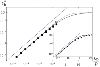
Figure 1: Efficiency at maximum power $\epsilon^{*}_{\rm h}$ for diffusiophoresis in non-ionic solutes. ($\square$): Van der Waals attraction $\Psi(y)=-16/9\,A\,a^{3}R^{3}y^{-3}(y+2R)^{-3}$ where $A=1\,kT$ and $a$ is the solute radius. $a/R=\left[10^{-4}\ldots 0.1\right]$ and attraction is truncated at $y=a$. Concentration gradient is established externally. ($\blacksquare$): Same $\Psi(y)$ as before but concentration gradient is produced by a Janus particle. ($\cdots\cdots$): Generic repulsion $\Psi(y)=kT\,\exp\left(-y/l\right)$ with $l/R=\left[10^{-4}\ldots 10^{2}\right]$. Concentration gradient is established externally. (——):  Same $\Psi(y)$ as before but concentration gradient is produced by a Janus particle. Inset: diffusiophoresis in an externally established gradient of ionic solutes and $\kappa^{-1}/R=\left[10^{-4}\ldots 10^{2}\right]$. ($\bullet\,\bullet\,\bullet$):  $q=0.1,\,\nu=0$. ($\circ\,\circ\,\circ$):  $q=-0.5,\,\nu=10$. (——):  $q=0.1,\,\nu=1$.

Swimming speed.–

The energetic differences of micro- and nano-swimmers are accompanied by differences in the swimming speed. As a simple example, for micro-swimmers in neutral solute with $\mathbf{F}_{\rm m}=0$ one has $V\sim\frac{kT}{\eta}\,l^{2}\left(\nabla c_{1}\right)|_{r\rightarrow\infty}$ anderson1989colloid . However for swimmers with $l\gg R$ we find the scaling $V\sim\frac{kT}{\eta}\,\frac{l^{3}}{R}\left(\nabla c_{1}\right)|_{r\rightarrow\infty}$ Sabass2010 . Hence, aside from efficiency, nano-swimmers are qualitatively different from micro-swimmers in that their size can matter for their mobility.

Conclusion.–

Although phoretic effects are known for more than a century their energetic aspects have hardly been explored. In this letter we make an attempt in this direction by suggesting a generic scaling relation for the efficiency of surface-driven motion. It provides a widely applicable and simple concept to estimate hydrodynamic efficency without detailed knowledge of the system. Further, we show with analytical and numerical calculations that phoretic nano-swimmers offer energetic advantages; in particular with ionic solutes, where the Debye length can be tuned. Taken together, we see inspiring perspectives for artificial nanomotors which, reminiscent of actual biological motors, could possibly move not only in a controllable but also in an efficient way.

References

- (1) E. Lauga and T. R. Powers, Rep. Progr. Phys. 72, 096601 (2009)
- (2) J. L. Anderson, Annu. Rev. Fluid Mech. 21, 61 (1989)
- (3) R. Golestanian, T. B. Liverpool, and A. Ajdari, Phys. Rev. Lett. 94, 220801 (2005)
- (4) P. Dhar et al., Nano Lett. 6, 66 (2006)
- (5) J.R. Howse et al., Phys. Rev. Lett. 99, 48102 (2007)
- (6) G. Rückner and R. Kapral, Phys.Rev. Lett. 98, 150603 (2007)
- (7) M. Popescu, S. Dietrich, and G. Oshanin, J. Chem. Phys. 130, 194702 (2009)
- (8) F. Jülicher and J. Prost, Eur. Phys. J. E 29, 27 (2009)
- (9) J. Palacci et al., Phys. Rev. Lett. 104, 138302 (2010)
- (10) F. Jülicher, A. Ajdari, and J. Prost, Rev. Mod. Phys. 69, 1269 (1997)
- (11) H. A. Stone and A. D. T. Samuel, Phys. Rev. Lett. 77, 4102 (1996)
- (12) J. E. Avron, O. Gat, and O. Kenneth, Phys. Rev. Lett. 93, 186001 (2004)
- (13) J. Teran, L. Fauci, and M. Shelley, Phys. Rev. Lett. 104, 038101 (2010)
- (14) J. L. Anderson and D. C. Prieve, Sep. Purif. Methods 13, 67 (1984)
- (15) P. E. Lammert, J. Prost, and R. Bruinsma, J. Theor. Biol. 178, 387 (1996)
- (16) J. R. Blake, J. Fluid Mech. 46, 199 (1971)
- (17) J. Happel and H. Brenner, Low Reynolds number hydrodynamics (Martinus Nijhoff, 1983)
- (18) M. Teubner, J. Chem. Phys. 76, 5564 (1982)
- (19) C. Van den Broeck, Phys. Rev. Lett. 95, 190602 (2005)
- (20) H. J. Keh and Y. K. Wei, Langmuir 16, 5289 (2000)
- (21) D. C. Prieve et al., J. Fluid Mech. 148, 247 (1984)
- (22) For non ionic solutes: . For ionic solutes: with reduced diffusion constant .
- (23) In ionic solutes with .
- (24) .
- (25) P. O. Staffeld and J. A. Quinn, J. Colloid Interface Sci. 130, 88 (1989)
- (26) A. Ajdari and L. Bocquet, Phys. Rev. Lett. 96, 186102 (2006)
- (27) B. Sabass and U. Seifert, to be published.