Intrinsic stationarity for vector quantization: Foundation of dual quantization

Abstract

We develop a new approach to vector quantization, which guarantees an intrinsic stationarity property that also holds, in contrast to regular quantization, for non-optimal quantization grids. This goal is achieved by replacing the usual nearest neighbor projection operator for Voronoi quantization by a random splitting operator, which maps the random source to the vertices of a triangle of $d$-simplex. In the quadratic Euclidean case, it is shown that these triangles or $d$-simplices make up a Delaunay triangulation of the underlying grid.

Furthermore, we prove the existence of an optimal grid for this Delaunay – or dual – quantization procedure. We also provide a stochastic optimization method to compute such optimal grids, here for higher dimensional uniform and normal distributions. A crucial feature of this new approach is the fact that it automatically leads to a second order quadrature formula for computing expectations, regardless of the optimality of the underlying grid.

Keywords: Quantization, Stationarity, Voronoi tessellation, Delaunay triangulation, Numerical integration.

MSC 2010: 60F25, 65C50, 65D32

1 Introduction and motivation

Quantization of random variables aims at finding the best $p$-th mean approximation to a random vector (r.v.) $X:(\Omega,\mathcal{S},\mathbb{P})\to(\mathbb{R}^{d},\mathcal{B}^{d})$ and $\mathbb{R}^{d}$ equipped with a norm $\lVert\cdot\rVert$. That means, for $X\in L^{p}_{\mathbb{R}^{d}}(\mathbb{P}),\,p>0$, that we have to minimize

$$\mathbb{E}\min_{x\in\Gamma}\lVert X-x\rVert^{p}$$ (1)

over all finite grids $\Gamma\subset\mathbb{R}^{d}$ of a given size (the term grid is a convenient synonym for nonempty finite subset of $\mathbb{R}^{d}$). This problem has its origin in the fields of signal processing in the late 1940s. A mathematically rigorous and comprehensive exposition of this topic can be found in the book of Graf and Luschgy [7].

Using the nearest neighbor projection, we are able to construct a random variable $\widehat{X}^{\Gamma}$, which achieves the minimum in (1). Such an approximation, which is called Voronoi quantization, has been successfully applied to various problems in applied probability theory and mathematical finance, $e.g.$ multi-asset American/Bermudan style options pricing and $\delta$-hedging (see [1, 2]), swing options, supply gas contract, on energy markets (Stochastic control) (see [3, 4, 5]), nonlinear filtering method for stochastic volatility estimation (see [10, 14, 16, 17]), discretization of SPDE’s (stochastic Zakai and McKean-Vlasov equations) (see [6]).

Especially we may use optimal quantizations to establish numerical cubature formulas, $i.e.$ to approximate $\mathbb{E}F(X)$ by

$$\mathbb{E}F(\widehat{X}^{\Gamma})=\sum_{x\in\Gamma}w_{x}\cdot F(x),$$

where $w_{x}=\mathbb{P}(\widehat{X}^{\Gamma}=x)$.

Such a cubature formula is known to be optimal in the class of Lipschitz functionals and it holds for a Lipschitz functional $F$ (with Lipschitz ratio $[F]_{\text{Lip}}$)

$$\lvert\mathbb{E}F(X)-\mathbb{E}F(\widehat{X}^{\Gamma})\rvert\leq[F]_{\text{Lip}}\;\mathbb{E}\lVert X-\widehat{X}^{\Gamma}\rVert.$$ (2)

If $F$ exhibits a bit more smoothness, $i.e.$ is differentiable with Lipschitz continuous differential $F^{\prime}$ and $\widehat{X}^{\Gamma}$ fulfills the so-called stationarity property

$$\mathbb{E}\bigl{(}X\,|\,\widehat{X}^{\Gamma}\bigr{)}=\widehat{X}^{\Gamma},$$ (3)

we can derive by means of a Taylor expansion the second order rate

$$\lvert\mathbb{E}F(X)-\mathbb{E}F(\widehat{X}^{\Gamma})\rvert\leq[F^{\prime}]_{\text{Lip}}\;\mathbb{E}\lVert X-\widehat{X}^{\Gamma}\rVert^{2}.$$

Unfortunately, the stationarity property for the Voronoi quantization $\widehat{X}^{\Gamma}$ is a rather fragile object, since it only holds for grids $\Gamma$ which are especially tailored and optimized for the distribution of $X$.

That means, that if a grid $\Gamma$, which has been originally constructed and optimized for $X$, is employed to approximate a r.v. $Y$ which only slightly differs from $X$, then $\Gamma$ might be still an arbitrary good quantization for $Y$, $i.e.$ $\mathbb{E}\lVert Y-\widehat{Y}^{\Gamma}\rVert^{p}$ is very close to the optimal quantization error, but the stationarity property (3) is in general violated. Thus, only the first order bound (2) is in this case valid for a cubature formula based on a Voronoi quantization of $Y$.

In this paper, we look for an alternative to the nearest neighbor projection operator and the Voronoi quantization, which will be capable of preserving some stationarity property in the above setting. In order to achieve this, we pass on to a product space $(\Omega_{0}\times\Omega,{\mathcal{S}}_{0}\otimes\mathcal{S},\mathbb{P}_{0}\otimes\mathbb{P})$ and introduce a random splitting operator $\mathcal{J}_{\Gamma}:\Omega_{0}\times\mathbb{R}^{d}\to\Gamma$, which satisfies

$$\mathbb{E}(\mathcal{J}_{\Gamma}(Y)|Y)=Y$$

for any $\mathbb{R}^{d}$-valued r.v. $Y$ defined on $(\Omega,\mathcal{S},\mathbb{P})$ such that $\operatorname{supp}(\mathbb{P}_{Y})\subset\operatorname{conv}(\Gamma)$ where $\operatorname{supp}(\mathbb{P}_{Y})$ and $\operatorname{conv}(\Gamma)$ denote the support of the distribution $\mathbb{P}_{Y}$ and the convex hull of $\Gamma$ respectively. Note that this implies that $Y$ is compactly supported. As a matter of facts, such an operator fulfills the so-called intrinsic stationarity property

$$\mathbb{E}(\mathcal{J}_{\Gamma}(\xi))=\xi,\qquad\xi\in\operatorname{conv}(\Gamma).$$ (4)

Although this stationarity differs from the one defined above, one may again derive a second order error bound for a differentiable function $F$ with Lipschitz derivative

$$\lvert\mathbb{E}\,F(Y)-\mathbb{E}F(\mathcal{J}_{\Gamma}(Y))\rvert\leq[F^{\prime}]_{\text{Lip}}\;\mathbb{E}\lVert Y-\mathcal{J}_{\Gamma}(Y)\rVert^{2}$$

which now holds for any r.v. $Y$ regardless of the grid $\Gamma$, except satisfying $\operatorname{supp}(\mathbb{P}_{Y})\subset\operatorname{conv}(\Gamma)$.

On our way, we will make the connection with functional approximation by noting that the functional operator related to ${\cal J}_{\Gamma}$ defined by

$$\mathbb{J}_{\Gamma}(F):=\Big{(}\xi\longmapsto\mathbb{E}_{\mathbb{P}_{0}}F\big{(}{\cal J}_{\Gamma}(\omega_{0},\xi)\big{)}\Big{)}$$

is in standard situations a (classical) continuous piecewise affine interpolation approximation of $F$.

One may naturally ask at this stage for the best possible approximation power of $\mathcal{J}_{\Gamma}(X)$ to $X$, $i.e.$ minimize the $p$-th power mean error

$$\mathbb{E}\lVert X-\mathcal{J}_{\Gamma}(X)\rVert^{p}$$

over all grids of size not exceeding $n$ and all random operators $\mathcal{J}_{\Gamma}$ fulfilling the intrinsic stationarity property (4).

This means, that we will deal for $n\in\mathbb{N}$ with the mean error modulus

$$\begin{split}d^{p}_{n}(X)=\inf\bigl{\{}\mathbb{E}\lVert X-\mathcal{J}_{\Gamma}(X)\rVert^{p}:&\,\Gamma\subset\mathbb{R}^{d},\lvert\Gamma\rvert\leq n,\,\operatorname{supp}(\mathbb{P}_{X})\subset\operatorname{conv}(\Gamma),\\ &\quad\mathcal{J}_{\Gamma}:\Omega_{0}\times\mathbb{R}^{d}\to\Gamma\text{ intrinsic stationary}\bigr{\}}\end{split}$$ (5)

where $|\Gamma|$ denotes the cardinality of $\Gamma$.

It will turn out in Section 2 that the problem of finding an optimal random operator $\mathcal{J}_{\Gamma}$ for a grid $\Gamma=\{x_{1},\ldots,x_{k}\},k\leq n$, is equivalent to solving the Linear Programming problem

$$\underset{\text{s.t. }\left[\begin{smallmatrix}x_{1}&\ldots&x_{k}\\ 1&\ldots&1\\ \end{smallmatrix}\right]\lambda=\left[\begin{smallmatrix}X(\omega)\\ 1\\ \end{smallmatrix}\right],\,\lambda\geq 0}{\min_{\lambda\in\mathbb{R}^{n}}\sum_{i=1}^{k}\lambda_{i}\,\lVert X(\omega)-x_{i}\rVert^{p}}$$ (6)

where $\displaystyle\left[\begin{smallmatrix}x_{1}&\ldots&x_{k}\\ 1&\ldots&1\\ \end{smallmatrix}\right]\lambda=\left[\begin{smallmatrix}\sum_{1\leq i\leq k}\lambda_{i}x_{i}\\ \sum_{1\leq i\leq k}\lambda_{i}\\ \end{smallmatrix}\right]$. Defining the local dual quantization function as

$$F^{p}(\xi,\Gamma)=\underset{\text{s.t. }\left[\begin{smallmatrix}x_{1}&\ldots&x_{k}\\ 1&\ldots&1\\ \end{smallmatrix}\right]\lambda=\left[\begin{smallmatrix}\xi\\ 1\\ \end{smallmatrix}\right],\,\lambda\geq 0}{\min_{\lambda\in\mathbb{R}^{n}}\sum_{i=1}^{k}\lambda_{i}\,\lVert\xi-x_{i}\rVert^{p}},$$

we will show that

$$d^{p}_{n}(X)=\inf\bigl{\{}\mathbb{E}\,F^{p}(X;\Gamma):\Gamma\subset\mathbb{R}^{d},\lvert\Gamma\rvert\leq n\bigr{\}}.$$ (7)

This means, that the dual quantization problem actually consists of two phases: during the first one we have to locally solve the optimization problem (6), whereas phase two, which consists of the global optimization over all possible grids in (7), is the more involved problem. It is highly non-linear and contains a probabilistic component by contrast to phase one which can be considered more or less as deterministic.

Moreover, we will see in section 3 that the solution to the Linear Programming (6) is in the quadratic Euclidean case completely determined by the Delaunay triangulation spanned by $\Gamma$ and this structure is, in the graph theoretic sense, the dual counterpart of the Voronoi diagram, on which regular quantization is based. That is actually also the reason, why we call this new approach dual or Delaunay quantization.

In section 2, we propose an extension of the dual quantization idea to non-compactly supported random variables. For those and the compactly supported r.v.’s we prove the existence of optimal quantizers in section 4, $i.e.$ the fact, that there are sets $\Gamma$, which actually achieve the infimum in (5). Finally, in section 5, we give numerical illustrations of some optimal dual quantizers and numerical procedures to generate them.

In a companion paper [12], we establish the counterpart of the celebrated Zador theorem for regular vector quantization: namely we elucidate the sharp rate for the mean dual quantization error modulus defined in section 2 below.

We also provide in [12] a non-asymptotic version of this theorem, which corresponds to the Pierce Lemma.

First numerical applications of dual quantization to Finance have been developed in a second companion paper [13], especially for the pricing of American style derivatives like Bermuda and swing options.

Notation: $\bullet$ $u^{T}$ will denote the transpose of the column vector $u\in\mathbb{R}^{d}$.

$\bullet$ Let $u=(u_{1},\ldots,u_{d})\!\in\mathbb{R}^{d}$, we write $u\geq 0$ (resp. $>0$) if $u_{i}\geq 0$ (resp $>0$), $i=1,\ldots,d$.

$\bullet$ $\Delta_{d}:=\{x=(x^{0},\ldots,x^{d})\!\in\mathbb{R}_{+}^{d+1},\;x^{0}+\cdots+x^{d}=1\}$ denotes the canonical simplex of $\mathbb{R}^{d+1}$.

$\bullet$ $B_{\lVert.\rVert}(x_{0},r)$ is the closed ball of center $x_{0}\!\in\mathbb{R}^{d}$ and radius $r\geq 0$ in $(\mathbb{R}^{d},\lVert.\rVert)$.

$\bullet$ ${\rm rk}(M)$ denotes the rank of the matrix $M$.

$\bullet$ $\mathbbm{1}_{A}$ denotes the indicator function of the set $A$, $|A|$ its cardinality.

$\bullet$ If $A\subset E$, $E$ $\mathbb{R}$-vector space, $\operatorname{span}A$ denotes the sub-vector space spanned by $A$.

$\bullet$ Let $(A_{n})_{n\geq 1}$ be a sequence of sets: $\limsup_{n}A_{n}:=\cap_{n}\cup_{k\geq n}A_{k}$ and $\liminf_{n}A_{n}:=\cup_{n}\cap_{k\geq n}A_{k}$.

$\bullet$ $\lambda^{d}$ denotes the Lebesgue measure on ($\mathbb{R}^{d},\mathfrak{B}(\mathbb{R}^{d}))$ (Borel $\sigma$-field).

2 Dual quantization and intrinsic stationarity

First, we briefly recall the definition of the “regular” vector quantization problem for a r.v. $X:(\Omega,\mathcal{S},\mathbb{P})\to(\mathbb{R}^{d},\mathcal{B}^{d})$ and $\mathbb{R}^{d}$ equipped with a norm $\lVert\cdot\rVert$.

Definition 1.

Let $X\in L^{p}_{\mathbb{R}^{d}}(\mathbb{P})$ for some $p\in[1,+\infty)$.

1. We define the (regular) $L^{p}$-mean quantization error for a grid $\Gamma=\{x_{1},\ldots,x_{n}\}\subset\mathbb{R}^{d}$ as

   $$e_{p}(X;\Gamma)=\bigl{\lVert}\min_{1\leq i\leq k}\lVert X-x_{i}\rVert\bigr{\rVert}_{L^{p}}=\bigl{(}\mathbb{E}\min_{1\leq i\leq n}\lVert X-x_{i}\rVert^{p}\bigr{)}^{1/p},$$

2. The optimal regular quantization error, which can be achieved by a grid $\Gamma$ of size not exceeding $n\in\mathbb{N}$, is given by

   $$e_{n,p}(X)=\inf\bigl{\{}e_{p}(X;\Gamma):\Gamma\subset\mathbb{R}^{d},\lvert\Gamma\rvert\leq n\bigr{\}}.$$

Remark.

Since we will frequently consider the $p$-th power of $e_{p}(X;\Gamma)$ and $e_{n,p}(X)$, we will drop a duplicate index $p$ and write, e.g. $e_{n}^{p}(X)$ instead of $e_{n,p}^{p}(X)$.

It can be shown, that (at least) one optimal quantizer actually exists, $i.e.$ for every $n\in\mathbb{N}$ there is a grid $\Gamma\subset\mathbb{R}^{d}$ with $\lvert\Gamma\rvert\leq n$ such that

$$e_{p}(X;\Gamma)=e_{n,p}(X).$$

Moreover, this definition of the optimal quantization error is in fact equivalent to defining $e_{n}^{p}(X)$ as the best approximation error which can be achieved by a Borel transformation or by a discrete r.v. $\widehat{X}$ taking at most $n$ values.

Proposition 1.

Let $X\in L^{p}_{\mathbb{R}^{d}}(\mathbb{P}),\,n\in\mathbb{N}$. Then

$$\begin{split}e^{p}_{n}(X)&=\inf\bigl{\{}\mathbb{E}\lVert X-f(X)\rVert^{p}:f:\mathbb{R}^{d}\to\mathbb{R}\text{ Borel measurable},\lvert f(\mathbb{R}^{d})\rvert\leq n\bigr{\}}\\ &=\inf\bigl{\{}\mathbb{E}\lVert X-\widehat{X}\rVert^{p}:\widehat{X}\text{ is a r.v. with }\lvert\widehat{X}(\Omega)\rvert\leq n\bigr{\}}.\end{split}$$

The proof of this proposition is based on the construction of a Voronoi quantization of a r.v. by means of the nearest neighbour projection.

Therefore, let $\Gamma=\{x_{1},\ldots,x_{n}\}\subset\mathbb{R}^{d}$ be a grid and denote by $(C_{i}(\Gamma))_{1\leq i\leq n}$ a Borel partition of $\mathbb{R}^{d}$ satisfying

$$C_{i}(\Gamma)\subset\bigl{\{}\xi\in\mathbb{R}^{d}:\lVert\xi-x_{i}\rVert\leq\min_{1\leq j\leq n}\lVert\xi-x_{j}\rVert\bigr{\}}.$$

Such a partition is called a Voronoi partition generated by $\Gamma$ and we may define the corresponding nearest neighbour projection as

$$\pi_{\Gamma}(\xi)=\sum_{1\leq i\leq n}x_{i}\mathbbm{1}_{C_{i}(\Gamma)}(\xi).$$

The discrete r.v.

$$\widehat{X}^{\Gamma,\text{Vor}}=\pi_{\Gamma}(X)=\sum_{1\leq i\leq n}x_{i}\mathbbm{1}_{C_{i}(\Gamma)}(X)$$

is called Voronoi Quantization induced by $\Gamma$ and satisfies

$$e_{p}^{p}(X;\Gamma)=\mathbb{E}\lVert X-\pi_{\Gamma}(X)\rVert^{p}.$$

As already mentioned in the introduction, the concept of stationarity plays an important role in the application of quantization. A quantization $\widehat{X}$ is said to be stationary for the r.v. $X$, if it satisfies

$$\mathbb{E}(X|\widehat{X})=\widehat{X}.$$ (8)

It is well known that in the quadratic Euclidean case, $i.e.$ $p=2$ and $\lVert\cdot\rVert$ is the Euclidean norm, any optimal quantization (a r.v. $\widehat{X}$ with $\lvert\widehat{X}(\Omega)\rvert\leq n$ and $\mathbb{E}\lVert X-\widehat{X}\rVert^{p}=e^{p}_{n}(X),$) fulfills this property (this is no longer true in the present form for $p\neq 2$ or non Eucidean norm, see [8]).

Moreover, this stationarity condition is equivalent to the first order optimality criterion of the optimization problem

$$\mathbb{E}\min_{1\leq i\leq n}\lVert X-x_{i}\rVert^{2}\to\min_{x_{1},\ldots,x_{n}\in\mathbb{R}^{d}},$$

$i.e.$ the Voronoi quantization $\widehat{X}^{\Gamma,\text{Vor}}$ of a grid $\Gamma=\{x_{1},\ldots,x_{n}\}\subset\mathbb{R}^{d}$ satisfies the stationarity property (8) for a r.v. $X$, whenever $\Gamma$ is a zero of the first order derivative of the mapping $(x_{1},\ldots,x_{n})\mapsto\mathbb{E}\min_{1\leq i\leq n}\lVert X-x_{i}\rVert^{2}$.

By means of this stationarity property (8), we can derive the following second order error bound for a cubature formula based on quantization.

Proposition 2.

Let $X\in L^{2}_{\mathbb{R}^{d}}(\mathbb{P})$ and assume that $F\in C^{1,1}(\mathbb{R}^{d})$ is differentiable with Lipschitz differential. If the quantization $\widehat{X}^{\Gamma}$ for a grid $\Gamma=\{x_{1},\ldots,x_{n}\}=\widehat{X}^{\Gamma}(\Omega),\,n\in\mathbb{N}$ satisfies

$$\mathbb{E}(X|\widehat{X}^{\Gamma})=\widehat{X}^{\Gamma},$$

then it holds for the cubature formula $\mathbb{E}\,F(\widehat{X}^{\Gamma})=\sum_{i=1}^{n}\mathbb{P}(\widehat{X}^{\Gamma}=x_{i})\cdot F(x_{i})$

$$\lvert\mathbb{E}\,F(X)-\mathbb{E}\,F(\widehat{X}^{\Gamma})\rvert\leq[F^{\prime}]_{\text{Lip}}\;\mathbb{E}\lVert X-\widehat{X}^{\Gamma}\rVert^{2}.$$

Proof.

From a Taylor expansion we obtain for $\widehat{X}=\widehat{X}^{\Gamma}$

$$\lvert F(X)-F(\widehat{X})-F^{\prime}(\widehat{X})(X-\widehat{X})\rvert\leq[F^{\prime}]_{\text{Lip}}\;\lVert X-\widehat{X}\rVert^{2},$$

so that taking conditional expectations and applying Jensen’s inequality yield

$$\lvert\mathbb{E}\bigl{(}F(X)|\widehat{X}\bigr{)}-F(\widehat{X})-\mathbb{E}\bigl{(}F^{\prime}(\widehat{X})(X-\widehat{X})|\widehat{X}\bigr{)}\rvert\leq[F^{\prime}]_{\text{Lip}}\;\mathbb{E}\bigl{(}\lVert X-\widehat{X}\rVert^{2}|\widehat{X}\bigr{)}.$$

The stationarity assumption then implies

$$\mathbb{E}\bigl{(}F^{\prime}(\widehat{X})(X-\widehat{X})|\widehat{X}\bigr{)}=F^{\prime}(\widehat{X})\,\mathbb{E}\bigl{(}(X-\widehat{X})|\widehat{X}\bigr{)}=0,$$

so that the assertion follows again from taking expectations and Jensen’s inequality. ∎

Unfortunately, the above stationarity is a rather fragile property, since it only holds for Voronoi quantizations, whose underlying grid is specifically optimized for the distribution of $X$. Thus, this stationarity will in general fail, as soon as we modify the underlying r.v. even only slightly. Nevertheless, there is a second way to derive the second order error bound of Proposition 2:

Assume that $\widehat{X}$ is a discrete r.v. satisfying a somewhat dual stationarity property

$$\mathbb{E}(\widehat{X}|X)=X.$$ (9)

In this case we can perform, as in the proof of Proposition 2, a Taylor expansion, but this time with respect to $X$. We then conclude from (9)

$$\mathbb{E}\bigl{(}F^{\prime}(X)(X-\widehat{X})|X\bigr{)}=0$$

so that finally the same assertion will hold.

As we will see later on, this stationarity condition will be intrinsically fulfilled by the dual quantization operator. Thus, this new approach will be be very robust with respect to changes in the underlying r.v.s, since it always preserves stationarity.

2.1 Definition of dual quantization

We define here the dual quantization error by means of the local dual quantization error $F_{p}$, since, doing so, we are able to introduce dual quantization along the lines of regular quantization. The stationarity property (9) will then appear as characterizing property of the Delaunay quantization and the dual quantization operator, the counterpart of Voronoi quantization and the nearest neighbour projection.

The equivalence of the following Definition 2 and (5) will be given in Theorem 2, which provides an analog statement for dual quantization to Proposition 1.

Without loss of generality assume from here on that

$$\operatorname{span}(\operatorname{supp}(\mathbb{P}_{X}))=\mathbb{R}^{d},$$

$i.e.$ $X$ is a true $d$-dimensional random variable. Otherwise we would reduce $d$. In the definitions below, we use the usual convention $\inf\{\emptyset\}=+\infty$.

Definition 2.

Let $X\in L^{p}_{\mathbb{R}^{d}}(\mathbb{P})$ for some $p\in[1,\infty)$.

$(a)$ The local dual quantization error induced by a grid $\Gamma=\{x_{1},\ldots,x_{n}\}\subset\mathbb{R}^{d}$ and $\xi\!\in\mathbb{R}^{d}$ is defined by

$$F_{p}(\xi;\Gamma)=\inf\left\{\Bigl{(}\sum_{1\leq i\leq n}\lambda_{i}\lVert\xi-x_{i}\rVert^{p}\Bigr{)}^{1/p}:\lambda_{i}\geq 0\text{ and }\sum_{1\leq i\leq n}\lambda_{i}x_{i}=\xi,\sum_{1\leq i\leq n}\!\!\lambda_{i}=1\right\}.$$

$(b)$ The $L^{p}$-mean dual quantization error for $X$ induced by the grid $\Gamma$ is then given by

$$d_{p}(X;\Gamma)=\lVert F_{p}(X;\Gamma)\rVert_{L^{p}}=\Bigl{(}\mathbb{E}\inf\Bigl{\{}\sum_{1\leq i\leq n}\lambda_{i}\lVert X-x_{i}\rVert^{p}:\lambda_{i}\geq 0,\sum_{1\leq i\leq n}\!\!\lambda_{i}x_{i}=X,\sum_{1\leq i\leq n}\!\!\lambda_{i}=1\Bigr{\}}\Bigr{)}^{1/p}.$$

$(c)$ The optimal dual quantization error, which can be achieved by a grid $\Gamma$ of size not exceeding $n$ will be denoted by

$$d_{n,p}(X)=\inf\bigl{\{}d_{p}(X;\Gamma):\Gamma\subset\mathbb{R}^{d},\lvert\Gamma\rvert\leq n\bigr{\}}.$$

Remarks. $\bullet$ Note that, like in the case of regular (Voronoi) quantization, the optimal dual quantization error depends actually only on the distribution of $X$.

$\bullet$ Note that $F_{p}(\xi,\Gamma)\geq{\rm dist}(\xi,\Gamma)$ and consequently $d_{p}(X,\Gamma)\geq e_{p}(X,\Gamma)$.

$\bullet$ In most cases we will deal with the $p$-th power of $F_{p},\,d_{p}$ and $d_{n,p}$. To avoid duplicating indices, we will write $F^{p},\,d^{p}$ and $d^{p}_{n}$ instead of $F_{p}^{p},\,d_{p}^{p}$ and $d_{n,p}^{p}$.

Denoting $\Gamma\!=\!\{x_{1},\ldots,x_{n}\}$, we recognize that $F^{p}(\xi;\Gamma)$ is given by the linear programming problem

$$\underset{\text{s.t. }\left[\begin{smallmatrix}x_{1}&\cdots&x_{n}\\ 1&\cdots&1\\ \end{smallmatrix}\right]\lambda=\left[\begin{smallmatrix}\xi\\ 1\\ \end{smallmatrix}\right],\,\lambda\geq 0}{\min_{\lambda\in\mathbb{R}^{n}}\sum_{i=1}^{n}\lambda_{i}\,\lVert\xi-x_{i}\rVert^{p}}.$$ (LP)

Clearly, we have $F^{p}(\xi;\Gamma)\geq 0$ for every $\xi\!\in\mathbb{R}^{d},\Gamma\subset\mathbb{R}^{d}$, so that it follows from the constraints

$$\left[\begin{matrix}x_{1}\cdots x_{n}\\ 1\cdots 1\end{matrix}\right]\lambda=\left[\begin{matrix}\xi\\ 1\end{matrix}\right],\quad\lambda\geq 0$$ (10)

that (LP) has a finite solution if and only if $\xi\in\operatorname{conv}(\Gamma)$.

Proposition 3.

$(a)$ Let $p\!\in[1,+\infty)$ and assume $\operatorname{supp}(\mathbb{P}_{X})$ is compact. Then $d_{n,p}(X)<+\infty$ if and only if $n\geq d+1$.

$(b)$ Let $p\!\in(1,+\infty)$. It holds

$$\{d_{p}(X;\,\cdot\,)<+\infty\}=\{\Gamma\subset\mathbb{R}^{d}:\operatorname{conv}(\Gamma)\supset\operatorname{supp}(\mathbb{P}_{X})\}.$$

Proof.

$(a)$ Let $\xi_{0}\!\in\operatorname{supp}(\mathbb{P}_{X})$ and $R>0$ such that ${\rm supp}\,\mathbb{P}_{X}\subset B_{\ell^{\infty}}(\xi_{0},\frac{R}{2})$ (closed ball w.r.t. the $\ell^{\infty}$-norm). Note that $[-\frac{R}{2},\frac{R}{2}]^{d}\subset-\frac{R}{2}\mbox{\bf 1}+R\,\Delta_{d}$ where $\Delta_{d}$ denotes the canonical simplex. Consequently

$$\operatorname{supp}(\mathbb{P}_{X})\subset\xi_{0}-\frac{R}{2}\mbox{\bf 1}+R\,\Delta_{d}=\operatorname{conv}(\Gamma_{0}),\;\Gamma_{0}=\{\xi_{0}-R/2+Re^{j},\;j=0,\ldots,d\}$$

where $e^{0}=0$ and $(e^{j})_{1\leq j\leq d}$ denotes the canonical basis of $\mathbb{R}^{d}$. Consequently

$$\forall\,\xi\!\in\operatorname{supp}(\mathbb{P}_{X}),\;F_{p}(\xi;\Gamma_{0})\leq\delta(\Gamma_{0})$$

where $\delta(A):=\sup_{x,y\in A}\lVert x-y\rVert$ denotes the diameter of $A$. More generally, for every grid $\Gamma$ such that $\operatorname{supp}(\mathbb{P}_{X})\subset\operatorname{conv}(\Gamma)$, $F_{p}(\xi;\Gamma)<+\infty$ for every $\xi\!\in{\rm supp}\,\mathbb{P}_{X}$.

Hence, for every $n\geq|\Gamma_{0}|=d+1$,

$$d_{n,p}(X)\leq\delta(\Gamma_{0}).$$

If $n\leq d$, the convex hull of a grid $\Gamma$ cannot contain $\operatorname{supp}(\mathbb{P}_{X})$: if so it contains its convex hull ${\rm conv}({\rm supp}\mathbb{P}_{X}))$ as well which is impossible since it has a nonempty interior whereas the dimension of $\operatorname{conv}(\Gamma)$ is at most $n-1$-dimensional.

$(b)$ It follows from what precedes that $d_{p}(X;\Gamma)<+\infty$ if $\operatorname{conv}(\Gamma)\supset\operatorname{supp}(\mathbb{P}_{X})$. Conversely, if $\operatorname{conv}(\Gamma)\not\supset\operatorname{supp}(\mathbb{P}_{X})$, there exists $\xi_{0}\!\in\operatorname{supp}(\mathbb{P}_{X})\setminus\operatorname{conv}(\Gamma)$. Let $\varepsilon_{0}>0$ such that $B(\xi_{0},\varepsilon_{0})\cap\operatorname{conv}(\Gamma)=\emptyset$. On $B(\xi_{0},\varepsilon_{0})$, $F_{p}(\,\cdot\,,\Gamma)\equiv+\infty$ and $\mathbb{P}_{X}(B(\xi_{0},\varepsilon_{0}))>0$, hence $d_{n,p}(X;\Gamma)=+\infty$. ∎

2.2 Preliminaries on the local dual quantization functional

Before we deal in detail with the dual quantization error for random variables, we have to derive some basic properties for the local dual quantization error functional $F_{p}$.

To alleviate notations, we introduce throughout the paper the abbreviations

$$A=\left[\begin{matrix}x_{1}\cdots x_{n}\\ 1\cdots 1\end{matrix}\right],\quad b=\left[\begin{matrix}\xi\\ 1\end{matrix}\right],\quad c=\left[\begin{matrix}\lVert\xi-x_{1}\rVert^{p}\\ \vdots\\ \lVert\xi-x_{n}\rVert^{p}\end{matrix}\right]$$

at least whenever $\Gamma$ and/or $\xi$ are fixed so that (LP) can be written as

$$\min_{\lambda\in\mathbb{R}^{k},\,A\lambda=b,\,\lambda\geq 0}\;\lambda^{T}c.$$

Moreover, for every set $I\subset\{1,\ldots,n\}$, $A_{I}=[a_{ij}]_{j\in I}$ will denote the submatrix of $A$ which columns correspond to the indices in $I$ and $c_{I}=[c_{i}]_{i\in I}$ will denote the subvector of $c$ which rows are determined by $I$. Finally, $\operatorname{aff.dim}(\Gamma)$ will denote the dimension of the affine manifold spanned by the grid $\Gamma$ in $\mathbb{R}^{d}$.

Since it follows from Proposition 3 that, for any grid $\Gamma=\{x_{1},\ldots,x_{n}\}\subset\mathbb{R}^{d}$ with $\operatorname{aff.dim}\{\Gamma\}<d$, $d_{p}(X;\Gamma)=+\infty$, we will restrict in the sequel to grids with $\operatorname{aff.dim}\{\Gamma\}=d$ or equivalently satsifying ${\rm rk}\left[\begin{smallmatrix}x_{1}&\cdots&x_{n}\\ 1&\cdots&1\\ \end{smallmatrix}\right]=d\!+\!1$. The following proposition is straightforward.

Proposition 4.

(see $e.g.$ [9], p33ff) For every $\xi\in\operatorname{conv}(\Gamma)$, (LP) has a solution $\lambda^{\ast}\in\mathbb{R}^{n}$, which is an extremal point of the compact set of linear constraints (10) so that ${\rm rk}\big{(}\left[\begin{smallmatrix}x_{i}\\ 1\end{smallmatrix}\right],\,i\!\in\{j\,|\,\lambda^{*}_{j}>0\}\big{)}$ are independent. Hence (by the incomplete basis theorem), there exists a fundamental basis $I^{\ast}\subset\{1,\ldots,n\}$, such that $\lvert I^{\ast}\rvert=d+1$, the columns $\left[\begin{smallmatrix}x_{j}\\ 1\end{smallmatrix}\right],\,j\!\in I^{\ast}$ are linearly independent and, after reordering the rows,

$$\lambda^{\ast}=\left[\begin{matrix}\lambda_{I^{*}}\\ 0\end{matrix}\right]\quad\mbox{where}\quad\lambda_{I^{*}}=A_{I^{\ast}}^{-1}b.$$ (11)

(Saying that $I^{\ast}$ is a basis rather than $\left[\begin{smallmatrix}x_{i}\\ 1\end{smallmatrix}\right],\,i\!\in I^{\ast}$, is a convenient abuse of notation). This means, that the columns of $\lambda^{\ast}$ corresponding to $I^{*}$ are given by $A_{I^{\ast}}^{-1}b$, the remaining ones being equal to $0$.

Consequently, the linear programming problem (LP) always admits a solution $\lambda^{\ast}$, whose non-zero components correspond to at most $d+1$ affinely independent points $x_{j}$ in $\Gamma$, $i.e.$ an optimal triangle in $\mathbb{R}^{2}$ or a $d$-simplex in $\mathbb{R}^{d}$.

Since the whole minimization problem can therefore be restricted to such triangles or $d$-simplices, we introduce the set of basis (or admissible indices) for a grid $\Gamma=\{x_{1},\ldots,x_{n}\}\subset\mathbb{R}^{d}$ as

$$\mathcal{I}(\Gamma)=\bigl{\{}I\subset\{1,\ldots,n\}:\lvert I\rvert=d+1\text{ and }\operatorname{rk}(A_{I})=d+1\bigr{\}}.$$

Moreover, we denote the optimality region for a basis $I\in\mathcal{I}(\Gamma)$ by

$$D_{I}(\Gamma)=\Biggl{\{}\xi\in\mathbb{R}^{d}:\lambda^{\ast}_{I}=A_{I}^{-1}\left[\begin{smallmatrix}\xi\\ 1\end{smallmatrix}\right]\geq 0\text{ and }\sum_{j\in I}\lambda^{\ast}_{j}\lVert\xi-x_{j}\rVert^{p}=F^{p}(\xi;\Gamma)\Biggr{\}}.$$

A useful reformulation of the above linear programming problem $(LP)$ is given by its dual version (see $e.g.$ [9], Theorem 3, p.91).

Proposition 5 (Duality).

The dual problem of (LP) reads

$$\begin{split}\underset{\text{s.t. }\left[\begin{smallmatrix}x_{1}&\cdots&x_{n}\\ 1&\cdots&1\\ \end{smallmatrix}\right]\lambda=\left[\begin{smallmatrix}\xi\\ 1\\ \end{smallmatrix}\right],\,\lambda\geq 0}{\min_{\lambda\in\mathbb{R}^{n}}\sum_{i=1}^{n}\lambda_{i}\,\lVert\xi-x_{i}\rVert^{p}}&=\underset{\text{ s.t. }\left[\begin{smallmatrix}x_{1}^{T}&1\\ \vdots&\vdots\\ x_{n}^{T}&1\\ \end{smallmatrix}\right]\left[\begin{smallmatrix}u_{1}\\ u_{2}\end{smallmatrix}\right]\leq\left[\begin{smallmatrix}\lVert\xi-x_{1}\rVert^{p}\\ \vdots\\ \lVert\xi-x_{n}\rVert^{p}\\ \end{smallmatrix}\right]}{\max_{u_{1}\in\mathbb{R}^{d},u_{2}\in\mathbb{R}}u_{1}^{T}\xi+u_{2}}\\ &=\max_{u\in\mathbb{R}^{d}}\min_{1\leq i\leq n}\bigl{\{}\lVert\xi-x_{i}\rVert^{p}+u^{T}(\xi-x_{i})\bigr{\}}.\end{split}$$ (DLP)

An important criterion to check, whether a triangle or a $d$-simplex in $\Gamma$ is optimal, is given by the following characterization of optimality in Linear Programs (see $e.g.$ [9], Theorem 3 and Remarks 6.4 and 6.5 that follow).

Proposition 6 (Optimality Conditions).

Let $\Gamma$ be a grid of $\mathbb{R}^{d}$ with $\operatorname{aff.dim}\Gamma=d$ and let $\xi\!\in{\rm conv}(\Gamma)$.

$(a)$ If a basis $I\in\mathcal{I}(\Gamma)$ is primal feasible, $i.e.$

$$\lambda_{I}=A_{I}^{-1}\left[\begin{smallmatrix}\xi\\ 1\end{smallmatrix}\right]\geq 0,$$

as well as dual feasible, $i.e.$

$$A^{T}u\leq\left[\begin{smallmatrix}\lVert\xi-x_{1}\rVert^{p}\\ \vdots\\ \lVert\xi-x_{n}\rVert^{p}\end{smallmatrix}\right]\quad\text{ for }\quad u=(A_{I}^{T})^{-1}c_{I},$$

then

$$\sum_{j\in I}\lambda_{j}\lVert\xi-x_{j}\rVert^{p}=\left[\begin{smallmatrix}\xi\\ 1\end{smallmatrix}\right]^{T}u.$$

Furthermore $\lambda_{I}$ and $u$ are optimal for (LP) resp. (DLP) and $I$ is called optimal basis.

$(b$) Conversely, if $I\in\mathcal{I}(\Gamma)$ is an optimal basis, which is additionally non-degenerate for (LP), $i.e.$ if there exist $\lambda\in\mathbb{R}^{k}$ and $u\in\mathbb{R}^{d+1}$ such that $\lambda_{I}=A_{I}^{-1}\left[\begin{smallmatrix}\xi\\ 1\end{smallmatrix}\right]>0$, $A^{T}u\leq c$ and $\displaystyle\sum_{j\in I}\lambda_{j}\lVert\xi-x_{j}\rVert^{p}=\left[\begin{smallmatrix}\xi\\ 1\end{smallmatrix}\right]^{T}u$, then it holds

$$A_{I}^{T}u=c_{I}.$$

Now we may derive the continuity of $F^{p}$ as a function of $\xi$ on $\operatorname{conv}(\Gamma)$.

Theorem 1.

Let $\Gamma=\{x_{1},\ldots,x_{n}\}\subset\mathbb{R}^{d},\,n\in\mathbb{N}$, be a fixed grid of size $k$. Then the function $f_{\Gamma}:\operatorname{conv}(\Gamma)\to\mathbb{R}$ defined by $f_{\Gamma}(\xi)=F^{p}(\xi;\Gamma)$ is continuous.

Proof.

The lower semi-continuity (l.s.c.) of $f_{\Gamma}$ follows directly from its dual representation

$$f_{\Gamma}(\xi)=\sup_{u\in\mathbb{R}^{d}}\min_{1\leq i\leq n}\bigl{\{}\lVert\xi-x_{i}\rVert^{p}+u^{T}(\xi-x_{i})\bigr{\}}$$

since the supremum of a family of continuous functions is l.s.c.

To establish the upper semi-continuity, we proceed as follows. Let $\xi,\xi^{n}\in\operatorname{conv}(\Gamma)$ such that $\xi^{n}\to\xi$ as $n\to\infty$. Since $\xi,\,\xi^{n}\in\operatorname{conv}(\Gamma)$, we know that $f_{\Gamma}(\xi)$ and $\displaystyle\limsup_{n\to\infty}f_{\Gamma}(\xi^{n})$ are upper bounded by $\delta(\Gamma)$ hence finite. Moreover, there is an $I^{\ast}\in\mathcal{I}(\Gamma)$ such that $(x_{i})_{i\in I^{*}}$ is an affine basis and such that

$$f_{\Gamma}(\xi)=\sum_{i\in I^{\ast}}\lambda^{\ast}_{i}\lVert\xi-x_{i}\rVert^{p}\quad\text{ and }\quad\sum_{i\in I^{\ast}}\lambda^{\ast}_{i}x_{i}=\xi,\;\sum_{i\in I^{ast}}\lambda^{\ast}_{i}=1,\;\lambda^{\ast}_{i}\geq 0,\,i\!\in I^{\ast}.$$

Up to an extraction, still denoted $(f_{\Gamma}(\xi_{n}))_{n\geq 1}$, one may assume that in fact $f_{\Gamma}(\xi_{n})\to\limsup_{n}f_{\Gamma}(\xi_{n})$ and that there exists an index subset $I_{0}\subset\{1,\ldots,n\}$ such that, for every $n\geq 1$, $\xi_{n}\!\in{\rm conv}(\Gamma_{I_{0}})$ where $\Gamma_{I}:=\{x_{i},\,i\!\in I\}$. The convex hull being closed, $\xi\!\in{\rm conv}(\Gamma_{I_{0}})$. Hence there exists $(\lambda^{0}_{i})_{i\in I_{0}}$ such that

$$\xi=\sum_{i\in I_{0}}\lambda^{0}_{i}x_{i},\quad\sum_{i\in I_{0}}\lambda^{0}_{i}=1,\;\lambda^{0}_{i}\geq 0,\,i\!\in I_{0}.$$

Now let $\xi^{\prime}\!\in{\rm conv}(\Gamma_{I_{0}})$ $i.e.$ writing $\xi^{\prime}=\sum_{i\in I_{0}}\lambda^{\prime}_{i}x_{i}$, $\sum_{i\in I_{0}}\lambda^{\prime}_{i}=1$, $\lambda^{\prime}_{i}\geq 0$, $i\!\in I_{0}$. Let $i^{\prime}_{0}={\rm argmin}\Big{\{}\frac{\lambda^{\prime}_{i}}{\lambda^{0}_{i}},\;\lambda^{0}_{i}>0\Big{\}}$. Then

$$\xi^{\prime} = \sum_{i\in I_{0},i\neq i^{\prime}_{0}}\lambda^{\prime}_{i}x_{i}+\frac{\lambda^{\prime}_{i^{\prime}_{0}}}{\lambda^{0}_{i^{\prime}_{0}}}\big{(}\xi-\sum_{i\in I_{0},i\neq i^{\prime}_{0}}\lambda^{0}_{i}x_{i})\big{)}$$

$$= \sum_{i\in I_{0},i\neq i^{\prime}_{0}}\underbrace{\big{(}\lambda^{\prime}_{i}-\frac{\lambda^{\prime}_{i^{\prime}_{0}}}{\lambda^{0}_{i^{\prime}_{0}}}\lambda^{0}_{i}\big{)}}_{\geq 0}x_{i}+\frac{\lambda^{\prime}_{i^{\prime}_{0}}}{\lambda^{0}_{i^{\prime}_{0}}}\xi$$

where $\sum_{i\in I_{0},i\neq i^{\prime}_{0}}\big{(}\lambda^{\prime}_{i}-\frac{\lambda^{\prime}_{i^{\prime}_{0}}}{\lambda^{0}_{i^{\prime}_{0}}}\lambda^{0}_{i}\big{)}+\frac{\lambda^{\prime}_{i^{\prime}_{0}}}{\lambda^{0}_{i^{\prime}_{0}}}=(1-\lambda^{\prime}_{i^{\prime}_{0}})-\frac{\lambda^{\prime}_{i^{\prime}_{0}}}{\lambda^{0}_{i^{\prime}_{0}}}(1-\lambda^{0}_{i^{\prime}_{0}})+\frac{\lambda^{\prime}_{i^{\prime}_{0}}}{\lambda^{0}_{i^{\prime}_{0}}}=1$. Consequently $\xi^{\prime}\!\in{\rm conv}(\Gamma_{I_{0}\setminus\{i^{\prime}_{0}\}}\cup\{\xi\})$. Now, $I_{0}$ being finite, it follows that, up to a new extraction, one may assume that

$$\xi_{n}\!\in{\rm conv}(\Gamma_{I_{0}\setminus\{i_{0}\}}\cup\{\xi\})\quad\mbox{ for an $i_{0}\!\in I_{0}$.}$$

Case 1. If $\xi\notin{\rm aff}(\Gamma_{I_{0}\setminus\{i_{0}\}})$, then $\Gamma_{I_{0}\setminus\{i_{0}\}}\cup\{\xi\}$ is affinely free and then $\xi_{n}$ writes uniquely

$$\xi_{n}=\mu^{n}\xi+\sum_{i\in I_{0}\setminus\{i_{0}\}}\mu^{n}_{i}x_{i}$$

as a (convex) linear combination. Since $\xi_{n}\to\xi$, one has owing to compactness and uniqueness arguments that $\mu^{n}_{i}\to 0$ $i\!\in I_{0}\setminus\{i_{0}\}$ and $\mu^{n}\to 1$ as $n\to\infty$. One derives that

$$\xi_{n}=\sum_{i\in I_{0}\setminus\{i_{0}\}}\mu^{n}_{i}x_{i}+\sum_{j\in I^{\ast}}\mu^{n}\lambda^{\ast}_{j}x_{j}$$

so that

$$f_{\Gamma}(\xi_{n})\leq\sum_{i\in I_{0}\setminus\{i_{0}\}}\mu^{n}_{i}\|x_{i}-\xi_{n}\|^{p}+\sum_{j\in I^{\ast}}\mu^{n}\lambda^{\ast}_{j}\|x_{j}-\xi_{n}\|^{p}$$

which implies in turn

$$\lim_{n}f_{\Gamma}(\xi_{n})\leq\sum_{i\in I_{0}\setminus\{i_{0}\}}\,0\,+1\times f_{\Gamma}(\xi).$$

Case 2. If $\xi\in{\rm aff}(\Gamma_{I_{0}\setminus\{i_{0}\}})$ then $\xi\in\operatorname{conv}(\Gamma_{I_{0}\setminus\{i_{0}\}})$ by uniqueness of barycentric coordinates in the affine basis $\Gamma_{I_{0}\setminus\{i_{0}\}}$. Then $\xi_{n}$, $\xi\!\in{\rm conv}(\Gamma\setminus\{i_{0}\})$ and we can repeat the above procedure to reduce again $I_{0}\setminus\{i_{0}\}$ into $I_{0}\setminus\{i_{0},i_{1}\}$ until $\Gamma\setminus\{i_{0},i_{1},\ldots,i_{p}\}$ becomes affinely free. If so the same reasoning as above completes the proof. If it never occurs, this means that $\xi_{n}=\xi$ for every $n\geq 1$ which trivially solves the problem. ∎

We can now state the main result about the optimality regions $D_{I}(\Gamma)$.

Proposition 7.

(a) For every $I\in\mathcal{I}(\Gamma)$, $\{x_{j}:j\in I\}\,\subset\,D_{I}(\Gamma)\subset\,\operatorname{conv}\{x_{j}:j\in I\}$, $D_{I}(\Gamma)$ is closed and therefore a Borel set.

(b) The family $\bigl{(}D_{I}(\Gamma)\bigr{)}_{I\in\mathcal{I}(\Gamma)}$ makes up a Borel measurable covering of $\operatorname{conv}(\Gamma)$.

Proof.

$(a)$ The first inclusion is obvious (set $\xi=x_{j}$, $\lambda_{j}=1$) and the second one follows directly from the definition of $D_{I}(\Gamma)$. To recognize that $D_{I}(\Gamma)$ is closed, note that, owing to Theorem 1, the mappings $\xi\mapsto\sum_{j\in I}\lambda^{\ast}_{j}\lVert\xi-x_{j}\rVert^{p}$ and $\xi\mapsto F^{p}(\xi;\Gamma)$ are continuous.

$(b)$ Since (LP) has a solution for every $\xi\in\operatorname{conv}(\Gamma)$, we derive from Proposition 4 that $\displaystyle\bigcup_{I\in\mathcal{I}(\Gamma)}D_{I}(\Gamma)=\operatorname{conv}(\Gamma)$. ∎

2.3 Intrinsic stationarity

To establish the link between the above definition of dual quantization and stationary quantization rules, we have to precise the notion of intrinsic stationarity.

Definition 3.

$(a)$ Let $\Gamma\subset\mathbb{R}^{d}$ be a finite subset of $\mathbb{R}^{d}$ and let $(\Omega_{0},\mathcal{S}_{0},\mathbb{P}_{0})$ be a probability space. Any random operator $\mathcal{J}_{\Gamma}:(\Omega_{0}\times D,\mathcal{S}_{0}\otimes\mathcal{B}or(D))\to\Gamma$, $\operatorname{conv}(\Gamma)\subset D\subset\mathbb{R}^{d}$ is called a splitting operator (onto $\Gamma$).

A splitting operator on $\Gamma$ satisfying

$$\qquad\forall\xi\in\operatorname{conv}(\Gamma),\quad\mathbb{E}_{\mathbb{P}_{0}}\bigl{(}\mathcal{J}_{\Gamma}(.,\xi)\bigr{)}=\int_{\Omega_{0}}\mathcal{J}_{\Gamma}(\omega_{0},\xi)\,\mathbb{P}_{0}(d\omega_{0})=\xi$$

is called an intrinsic stationary splitting operator.

We will see in the next paragraph that $(\Omega_{0},\mathcal{S}_{0},\mathbb{P}_{0})$ can be modelled as an exogenous probability space in order to randomly “split” ($e.g.$ by simulation) a r.v. $X$, defined on the probability space of interest $(\Omega,\mathcal{S},\mathbb{P})$, between the points in $\Gamma$.

This new stationarity property is in fact equivalent to the dual stationarity property (9) on the product space $(\Omega_{0}\times\Omega,{\mathcal{S}}_{0}\otimes\mathcal{S},\mathbb{P}_{0}\otimes\mathbb{P})$ as emphasized by the following easy propositon.

Proposition 8.

Let $\operatorname{conv}(\Gamma)\subset D\subset\mathbb{R}^{d}$. A random splitting operator $\mathcal{J}_{\Gamma}:(\Omega_{0}\times D,\mathcal{S}_{0}\otimes\mathfrak{B}(D))\to\Gamma$ is intrinsic stationary, if and only if, for any r.v. $Y:(\Omega,\mathcal{S},\mathbb{P})\to(\mathbb{R}^{d},\mathcal{B}^{d})$ satisfying $\operatorname{supp}(\mathbb{P}_{Y})\subset\operatorname{conv}(\Gamma)$,

$$\mathbb{E}_{\mathbb{P}_{0}\otimes\mathbb{P}}\bigl{(}\mathcal{J}_{\Gamma}(Y)|Y\bigr{)}=Y\qquad\mathbb{P}_{0}\otimes\mathbb{P}\text{-a.s.}$$ (12)

where $\mathcal{J}_{\Gamma}$ and $Y$ are canonically extended onto $\Omega_{0}\times\Omega$ by setting $\mathcal{J}_{\Gamma}((\omega_{0},\omega),.)=\mathcal{J}_{\Gamma}(\omega_{0},.)$ and $Y(\omega_{0},\omega)=Y(\omega)$.

Proof.

The direct implication follows directly from Fubini’s theorem and Definition 3. For the reverse one simply set $Y\equiv\xi$. ∎

2.3.1 Dual quantization operator $\mathcal{J}_{\Gamma}^{\ast}$ and its interpolation counterpart $\mathbb{J}^{*}_{\Gamma}$

A way to define such an intrinsic stationary random splitting operator in an optimal manner is provided by the dual quantization operator $\mathcal{J}_{\Gamma}^{\ast}$.

Therefore, let $\Gamma=\{x_{1},\ldots,x_{n}\}\subset\mathbb{R}^{d},\,k\in\mathbb{N}$ and assume that $\operatorname{aff.dim}(\Gamma)=d$. Otherwise the dual quantization operator is not defined.

We then may choose a Borel partition $(C_{I}(\Gamma))_{I\in\mathcal{I}(\Gamma)}$ of $\operatorname{conv}(\Gamma)$ such that, for every $I\in\mathcal{I}(\Gamma)$,

$$C_{I}(\Gamma)\subset D_{I}(\Gamma)=\Bigl{\{}\xi\in\mathbb{R}^{d}:\lambda_{I^{\ast}}:=A_{I}^{-1}\left[\begin{smallmatrix}\xi\\ 1\end{smallmatrix}\right]\geq 0\text{ and }\sum_{j\in I}\lambda^{\ast}_{j}\lVert\xi-x_{j}\rVert^{p}=F^{p}(\xi;\Gamma)\Bigr{\}}$$

with the notations of (11). As a consequence, up to a reordering of rows, the Borel function

$$\lambda^{I}(\xi)=\left[\begin{matrix}A_{I}^{-1}\left[\begin{smallmatrix}\xi\\ 1\end{smallmatrix}\right]\\ 0\end{matrix}\right]$$ (13)

gives an optimal solution to $F^{p}(\xi;\Gamma)$ for every $\xi\in C_{I}$.

Now we are in position to define the dual quantization operator.

Definition 4 (Dual quantization operator).

Let $(\Omega_{0},\mathcal{S}_{0},\mathbb{P}_{0})=\bigl{(}[0,1],\mathfrak{B}([0,1]),\lambda^{1}\bigr{)}$ and let $U=\operatorname{Id}_{[0,1]}$ be the canonical random variable with $\mathcal{U}\bigl{(}[0,1]\bigr{)}$ distribution over the unit interval. The dual quantization operator $\mathcal{J}_{\Gamma}^{\ast}:\Omega_{0}\times\operatorname{conv}(\Gamma)\to\Gamma$ is then defined for every $(\omega_{0},\xi)\!\in\Omega_{0}\times\mathbb{R}^{d}$ by

$$\mathcal{J}_{\Gamma}^{\ast}(\omega_{0},\xi)=\sum_{I\in\mathcal{I}(\Gamma)}\Biggl{[}\sum_{i=1}^{n}x_{i}\cdot\mathbbm{1}_{\bigl{\{}\sum\limits_{j=1}^{i-1}\lambda^{I}_{j}(\xi)\,\leq\,U<\sum\limits_{j=1}^{i}\lambda^{I}_{j}(\xi)\bigr{\}}}(\omega_{0})\Biggr{]}\mathbbm{1}_{C_{I}(\Gamma)}(\xi).$$ (14)

The dual quantization operator is clearly an intrinsic stationary splitting operator. First

$$\forall\,I\!\in{\cal I}(\Gamma),\;\forall\,i\in I,\quad\mathbb{E}_{\mathbb{P}_{0}}\Big{(}\mathbbm{1}_{\bigl{\{}\sum\limits_{j=1}^{i-1}\lambda^{I}_{j}(\xi)\,\leq\,U<\sum\limits_{j=1}^{i}\lambda^{I}_{j}(\xi)\bigr{\}}}\Big{)}=\lambda_{i}^{I}(\xi).$$

On the other hand

$$\forall\xi\in C_{I}(\Gamma),\quad\sum_{i=1}^{n}\lambda_{i}^{I}(\xi)\,x_{i}=\xi,$$

so that $\mathcal{J}_{\Gamma}^{\ast}$ shares the intrinsic stationarity property:

$$\forall\xi\in\operatorname{conv}(\Gamma),\qquad\mathbb{E}_{\mathbb{P}_{0}}\bigl{(}\mathcal{J}_{\Gamma}^{\ast}(\xi)\bigr{)}=\sum_{I\in\mathcal{I}(\Gamma)}\Biggl{[}\sum_{i=1}^{n}\lambda_{i}^{I}(\xi)\,x_{i}\Biggr{]}\mathbbm{1}_{C_{I}(\Gamma)}(\xi)=\xi.$$

Remark. The $\mathfrak{B}([0,1])\otimes\mathfrak{B}(\operatorname{conv}(\Gamma))$-measurability of the dual quantization operator is an easy consequence of the facts that $C_{I}(\Gamma)$ are Borel sets and $\xi\mapsto\lambda^{I}(\xi)$ as defined by (13) is a continuous, hence Borel, function.

On the other hand, one easily checks that this construction also yields

$$\forall\,\xi\!\in\operatorname{conv}(\Gamma),\qquad\mathbb{E}_{\mathbb{P}_{0}}\lVert\xi-\mathcal{J}_{\Gamma}^{\ast}(\xi)\rVert^{p}=\sum_{i=1}^{n}\lambda^{I}_{i}(\xi)\|x_{i}-\xi\|^{p}=F^{p}(\xi;\Gamma).$$ (15)

Definition 5 (Companion interpolation operator).

The companion interpolation operator $\mathbb{J}^{*}_{\Gamma}$ is defined from ${\cal F}(\operatorname{conv}(\Gamma),\mathbb{R})=\{f:\operatorname{conv}(\Gamma)\to\mathbb{R}\}$ into itself by

$$\mathbb{J}^{*}_{\Gamma}(F)=\mathbb{E}_{\mathbb{P}_{0}}\Big{(}F\big{(}{\cal J}^{*}_{\Gamma}(\omega_{0},.)\big{)}\Big{)}=\sum_{I\in\mathcal{I}(\Gamma)}\left[\sum_{i\in I}\lambda^{I}_{i}\ F(x_{i})\right]\mathbbm{1}_{C_{I}(\Gamma)}$$ (16)

This operator $\mathbb{J}^{*}_{\Gamma}$ maps continuous functions into piecewise linear continuous functions and one clearly has

$$\mathbb{J}^{*}_{\Gamma}(F)(X)=\mathbb{E}\big{(}F(\mathcal{J}_{\Gamma}^{\ast}(X))\,|\,X\big{)}$$

so that $\mathbb{E}\big{(}\mathbb{J}^{*}_{\Gamma}(F)(X)\big{)}=\mathbb{E}\big{(}F(\mathcal{J}_{\Gamma}^{\ast}(X))\big{)}$.

Change of notation. From now on, we switch to the product space $(\Omega_{0}\times\Omega,{\mathcal{S}}_{0}\otimes\mathcal{S},\mathbb{P}_{0}\otimes\mathbb{P})$. (However, if no ambiguity, we will still use the symbols $\mathbb{P}$ and $\mathbb{E}$ to denote the probability and the expectation on this product space.) Doing so, we may assume that the intrinsic stationary splitting operator is independent of any “endogenous” r.v. defined on $(\Omega,\mathcal{S},\mathbb{P})$, canonically extended to $(\Omega_{0}\times\Omega,{\mathcal{S}}_{0}\otimes\mathcal{S},\mathbb{P}_{0}\otimes\mathbb{P})$ (which implies that the stationary property (12) holds).

2.3.2 Characterizations of the optimal dual quantization error

We use this operator to prove the analogous theorem for dual quantization to Proposition 1.

Theorem 2.

Let $X:(\Omega,{\cal S},\mathbb{P})\to\mathbb{R}^{d}$ be a r.v., let $p\!\in[1,\infty)$ and let $n\in\mathbb{N}$. Then

$$\begin{split}d_{n,p}(X)&=\inf\bigl{\{}\mathbb{E}\lVert X-\mathcal{J}_{\Gamma}(X)\rVert_{p}:\,\mathcal{J}_{\Gamma}:\Omega_{0}\times\mathbb{R}^{d}\to\Gamma,\,\Gamma\subset\mathbb{R}^{d},\text{ intrinsic stationary},\\ &\qquad\qquad\qquad\qquad\qquad\qquad\operatorname{supp}(\mathbb{P}_{X})\subset\operatorname{conv}(\Gamma),\,\lvert\Gamma\rvert\leq n\bigr{\}}\\ &=\inf\bigl{\{}\mathbb{E}\lVert X-\widehat{Y}\rVert_{p}:\widehat{Y}:(\Omega_{0}\times\Omega,{\mathcal{S}}_{0}\otimes\mathcal{S},\mathbb{P}_{0}\otimes\mathbb{P})\to\mathbb{R}^{d},\\ &\qquad\qquad\qquad\qquad\qquad\qquad\lvert\widehat{Y}(\Omega_{0}\times\Omega)\rvert\leq n,\,\mathbb{E}_{\mathbb{P}\otimes\mathbb{P}_{0}}(\widehat{Y}|X)=X\;\mathbb{P}\otimes\mathbb{P}_{0}\mbox{-}a.s.\bigr{\}}\leq+\infty.\end{split}$$

These quantities are finite iff $X\in L^{\infty}(\Omega,\mathcal{S},\mathbb{P})$ and $n\geq d+1$.

Proof.

First we show the inequality

$$\begin{split}d^{p}_{n}(X)\geq\inf\bigl{\{}\mathbb{E}\lVert X-\mathcal{J}_{\Gamma}(X)\rVert^{p}:&\,\mathcal{J}_{\Gamma}:\mathbb{R}^{d}\to\Gamma\text{ is intrinsic stationary},\\ &\operatorname{supp}(\mathbb{P}_{X})\subset\operatorname{conv}(\Gamma),\,\Gamma\subset\mathbb{R}^{d},\,\lvert\Gamma\rvert\leq n\bigr{\}}.\end{split}$$ (17)

We may assume that $d^{p}_{n}(X)<+\infty$ which implies the existence of a grid $\Gamma\in\mathbb{R}^{d}$ with $\lvert\Gamma\rvert\leq n$ and $d^{p}(X;\Gamma)<+\infty$ so that Proposition 3 implies $\operatorname{supp}(\mathbb{P}_{X})\subset\operatorname{conv}(\Gamma)$.

Hence, we choose a Borel partition $(C_{I}(\Gamma))_{I\in\mathcal{I}(\Gamma)}$ of $\operatorname{conv}(\Gamma)$ with $C_{I}(\Gamma)\subset D_{I}(\Gamma),\,I\in\mathcal{I}(\Gamma)$, so that the dual quantization operator $\mathcal{J}_{\Gamma}^{\ast}$ is well defined by (14) on $\operatorname{conv}(\Gamma)$. Let us still denote $\mathcal{J}_{\Gamma}^{\ast}$ its Borel extension by $0$ outside $\operatorname{conv}(\Gamma)$.

Owing to the independence of $X$ and $\mathcal{J}_{\Gamma}^{\ast}$ on $\Omega_{0}\times\Omega$, it holds

$$\mathbb{E}\bigl{(}\lVert\xi-\mathcal{J}_{\Gamma}^{\ast}(\xi)\rVert^{p}\bigr{)}_{|\xi=X}=\mathbb{E}\bigl{(}\lVert X-\mathcal{J}_{\Gamma}^{\ast}(X)\rVert^{p}\,|\,X\bigr{)}\qquad{a.s.},$$

so that we conclude from (15)

$$\begin{split}\mathbb{E}\,F^{p}(X;\Gamma)&=\mathbb{E}\bigl{[}\mathbb{E}\bigl{(}F^{p}(X;\Gamma)\,|\,X\bigr{)}\bigr{]}=\mathbb{E}\bigl{[}\mathbb{E}\bigl{(}F^{p}(\xi;\Gamma)\bigr{)}_{|\xi=X}\bigr{]}\\ &=\mathbb{E}\bigl{[}\mathbb{E}\bigl{(}\lVert\xi-\mathcal{J}_{\Gamma}^{\ast}(\xi)\rVert^{p}\bigr{)}_{|\xi=X}\bigr{]}=\mathbb{E}\bigl{[}\mathbb{E}\bigl{(}\lVert X-\mathcal{J}_{\Gamma}^{\ast}(X)\rVert^{p}\,|\,X\bigr{)}\bigr{]}\\ &=\mathbb{E}\lVert X-\mathcal{J}_{\Gamma}^{\ast}(X)\rVert^{p}.\end{split}$$

Since $\mathcal{J}_{\Gamma}^{\ast}$ is intrinsic stationary by construction, the first inequality (17) holds.

The second inequality

$$\begin{split}\inf\bigl{\{}&\mathbb{E}\lVert X-\mathcal{J}_{\Gamma}(X)\rVert^{p}:\,\mathcal{J}_{\Gamma}\text{ is intrinsic stationary},\,\operatorname{supp}(\mathbb{P}_{X})\subset\operatorname{conv}(\Gamma),\,\lvert\Gamma\rvert\leq n\bigr{\}}\\ &\geq\,\inf\bigl{\{}\mathbb{E}\lVert X-\widehat{Y}\rVert^{p}:\widehat{Y}\text{ is a r.v.},\lvert\widehat{Y}(\Omega_{0}\times\Omega)\rvert\leq n,\,\mathbb{E}(\widehat{Y}|X)=X\bigr{\}}\end{split}$$

follows directly from setting $\widehat{Y}=\mathcal{J}_{\Gamma}^{\ast}(X)$ in the case $\mathcal{J}_{\Gamma}^{\ast}$ exists and $\operatorname{supp}(\mathbb{P}_{X})\subset\operatorname{conv}(\Gamma)$. Otherwise, there is nothing to show.

To prove the reverse inequality, let us consider a r.v. $\widehat{Y}$ on $\Omega_{0}\times\Omega$ s.t. $\lvert\widehat{Y}(\Omega_{0}\times\Omega)\rvert\leq n$ and

$$\mathbb{E}(\widehat{Y}\,|\,X)=X\quad{a.s.}$$

Such r.v. do exist owing to what precedes. Let $\widehat{Y}(\Omega_{0}\times\Omega)=\{y_{1},\ldots,y_{k}\}$ with $k\leq n$ and let

$$\lambda_{i}=\Big{(}\xi\mapsto\mathbb{P}_{0}\otimes\mathbb{P}(\widehat{Y}=y_{i}\,|\,X=\xi)\Big{)}\circ X,\quad 1\leq i\leq k,$$

where the above mapping denotes a regular versions of the conditional expectation on $\mathbb{R}^{d}$ (so that $\lambda_{i}$ is $\mathcal{S}_{0}\otimes\mathcal{S}$-measurable), $i=1,\ldots,k$.

Hence, there exists a null set $N\in\mathcal{S}_{0}\otimes\mathcal{S}$ such that

$$\forall\bar{\omega}=(\omega_{0},\omega)\in N^{c},\quad\begin{cases}\sum\limits_{i=1}^{k}y_{i}\,\lambda_{i}(\bar{\omega})=\mathbb{E}(\widehat{Y}|X)(\bar{\omega})=X(\omega)\\ \sum\limits_{i=1}^{k}\lambda_{i}(\bar{\omega})=1\\ \lambda_{i}(\bar{\omega})\in[0,1],\;1\leq i\leq k.\end{cases}$$

Setting $\Gamma=\{y_{1},\ldots,y_{k}\}$, we get for every $\bar{\omega}\in N^{c}$

$$\begin{split}\mathbb{E}\bigl{(}\lVert X-\widehat{Y}\rVert^{p}\,|\,X\bigr{)}(\bar{\omega})&=\sum_{i=1}^{k}\lambda_{i}(\bar{\omega})\,\mathbb{E}\bigl{(}\lVert X-y_{i}\rVert^{p}\,|\,X\bigr{)}(\bar{\omega})=\sum_{i=1}^{k}\lambda_{i}(\bar{\omega})\,\lVert X(\omega)-y_{i}\rVert^{p}\\ &\geq F^{p}(X(\omega);\Gamma).\end{split}$$

Taking the expectation completes the proof. ∎

Remark. We necessarily need to define $\widehat{Y}$ on the larger product probability space $(\Omega_{0}\times\Omega,{\mathcal{S}}_{0}\otimes\mathcal{S},\mathbb{P}_{0}\otimes\mathbb{P})$ rather than only on $(\Omega,\mathcal{S},\mathbb{P})$, since $\mathcal{S}$ might not be fine enough to contain appropriated r.v.s $\widehat{Y}$ satisfying $\mathbb{E}(\widehat{Y}|X)=X$. E.g., if $\mathcal{S}=\sigma(X)$, $\widehat{Y}$ would be $\sigma(X)$-measurable so that $\mathbb{E}(\widehat{Y}|X)=\widehat{Y}$, intrinsic stationarity would become unreachable for general finite-valued r.v. $\widehat{Y}$.

2.3.3 Applications of intrinsic stationarity to cubature formulas

As a consequence of the above Theorem 2 we get the following theorem about cubature by dual quantization.

First, one must keep in mind as concerns functional approximation interpretation and numerical integration that $\mathbb{E}\big{(}\mathcal{J}_{\Gamma}^{\ast}(X\big{)})=\mathbb{E}\big{(}\mathbb{J}^{*}_{\Gamma}(F)(X)\big{)}$ and that the second expression based on the interpolation formula (16) may be more intuitive although, once the weights

$$p_{i}=\mathbb{P}(\mathcal{J}_{\Gamma}^{\ast}(X)=x_{i}),\;i=1,\ldots,n,$$

have been computed “off line” the cubature formula is of course more efficient in its aggregated form corresponding to $\mathbb{E}\big{(}\mathcal{J}_{\Gamma}^{\ast}(X\big{)})$. It is straightforward that if $F:\mathbb{R}^{d}\to\mathbb{R}$ is $\alpha$-Hölder continuous on $\operatorname{conv}(\Gamma)$, then (with obvious notations), if $\operatorname{conv}(\Gamma)\supset\operatorname{supp}(\mathbb{P}_{X})$,

$$\lvert\mathbb{E}\,F(X)-\mathbb{E}\big{(}\mathbb{J}^{*}_{\Gamma}(F)(X)\big{)}\rvert=\lvert\mathbb{E}\,F(X)-\mathbb{E}\,F(\mathcal{J}_{\Gamma}^{\ast}(X))\rvert\leq[F]_{\text{Lip}}\;\mathbb{E}\lVert X-\mathcal{J}_{\Gamma}^{\ast}(X)\rVert.$$

One may go further like with Voronoi quantization when $F$ is smoother, taking advantage of the stationarity property(satisfied here by any grid).

Proposition 9.

Let $X:(\Omega,{\cal S})\to\mathbb{R}^{d}$ be a r.v. with a compactly supported distribution $\mathbb{P}_{X}$. Let $\Gamma=\{x_{1},\ldots,x_{n}\}\subset\mathbb{R}^{d}$ be a grid with $\operatorname{conv}(\Gamma)\supset\operatorname{supp}(\mathbb{P}_{X})$. Then for every function $F:\mathbb{R}^{d}\to\mathbb{R}$, differentiable in the neighbourhood of $\operatorname{conv}(\Gamma)$, with Lipschitz continuous partial derivatives on $\operatorname{conv}(\Gamma)$, it holds for the cubature formula $\mathbb{E}\,F(\mathcal{J}_{\Gamma}^{\ast}(X))=\sum_{i=1}^{n}p_{i}\cdot F(x_{i})$

$$\lvert\mathbb{E}\,F(X)-\mathbb{E}\big{(}\mathbb{J}^{*}_{\Gamma}(F)(X)\big{)}\rvert=\lvert\mathbb{E}\,F(X)-\mathbb{E}\,F(\mathcal{J}_{\Gamma}^{\ast}(X))\rvert\leq[F^{\prime}]_{\text{Lip}}\;\mathbb{E}\lVert X-\mathcal{J}_{\Gamma}^{\ast}(X)\rVert^{2}.$$

Proof.

The result follows straightforwardly from taking the expectation in the Taylor expansion of $F$ at $X$ at the second order, namely

$$|F(\mathcal{J}_{\Gamma}^{\ast}(X))-F(X)-F^{\prime}(X).(\mathcal{J}_{\Gamma}^{\ast}(X)-X)|\leq[F^{\prime}]_{\text{Lip}}\lVert X-\mathcal{J}_{\Gamma}^{\ast}(X)\rVert^{2},$$

and applying the stationarity property $\mathbb{E}(\mathcal{J}_{\Gamma}^{\ast}(X)-X\,|\,X)=0$. ∎

Now assume that the integrand $F$ is a convex function. If $\widehat{X}^{\Gamma}$ is a Voronoi quantization which satisfies the regular stationarity property $\mathbb{E}(X|\widehat{X}^{\Gamma})=\widehat{X}^{\Gamma}$, it follows from Jensen’s inequality that $\mathbb{E}\,F(\widehat{X}^{\Gamma})$ yields a lower bound for the approximation of $\mathbb{E}\,F(X)$.

By contrast to that and exploiting the intrinsic stationarity of $\mathcal{J}_{\Gamma}^{\ast}$, a cubature formula based on $\mathcal{J}_{\Gamma}^{\ast}$ yields for convex functions $F$ an upper bound, which is now valid for any grid $\Gamma\subset\mathbb{R}^{d}$.

Proposition 10.

Let $X$ and $\Gamma$ be like in Proposition 9. Assume that $F:\operatorname{conv}(\Gamma)\to\mathbb{R}$ is convex. Then $\mathbb{J}^{*}_{\Gamma}(F)$ defines a convex function on $\operatorname{conv}(\Gamma)$ satisfying $\mathbb{J}^{*}_{\Gamma}(F)\geq F$. In particular

$$\mathbb{E}\big{(}\mathbb{J}^{*}_{\Gamma}(F)(X)\big{)}\geq\mathbb{E}\,F(X).$$

Proof. The inequality $\mathbb{J}^{*}_{\Gamma}(F)\geq F$ follows from the very definition (16) of $\mathbb{J}^{*}_{\Gamma}$. Its convexity is a consequence of its affinity on each $d$-simplex $C_{I}(\Gamma)$, and its coincidence with $F$ on $\Gamma$. $\Box$

Application to convex order. Dual quantization preserves the convex order on $\operatorname{conv}(\Gamma)$: if $X$ and $Y$ are two r.v. $a.s.$ taking values in $\operatorname{conv}(\Gamma)$ such that $X\preceq_{c}Y$ – $i.e.$ for every convex function $\varphi:\operatorname{conv}(\Gamma)\to\mathbb{R}$, $\mathbb{E}\,\varphi(X)\leq\mathbb{E}\,\varphi(Y)$ – then ${\cal J}_{\Gamma}^{*}(X)\preceq_{c}{\cal J}^{*}_{\Gamma}(y)$.

2.4 Upper bounds and product quantization

Proposition 11 (Scalar bound).

Let $\Gamma=\{x_{1},\ldots,x_{n}\}\subset\mathbb{R}$ with $x_{1}<\ldots<x_{n}$. Then

$$\forall\xi\in[x_{1},x_{n}],\qquad F^{p}(\xi,\Gamma)\leq\max_{1\leq i\leq n-1}\Bigl{(}\frac{x_{i+1}-x_{i}}{2}\Bigr{)}^{p}.$$

Proof.

If $\xi\in\Gamma$, then $F^{p}(\xi,\Gamma)=0$ and the assertion holds. Suppose now $\xi\in(x_{i},x_{i+1})$. Then $\xi=\lambda x_{i}+(1-\lambda)x_{i+1}$ and $\lambda=\frac{x_{i+1}-\xi}{x_{i+1}-x_{i}}$, so that

$$F^{p}(\xi,\Gamma)\leq\Bigl{(}\frac{x_{i+1}-\xi}{x_{i+1}-x_{i}}\Bigr{)}\lvert\xi-x_{i}\rvert^{p}+\Bigl{(}\frac{\xi-x_{i}}{x_{i+1}-x_{i}}\Bigr{)}\lvert\xi-x_{i+1}\rvert^{p}$$

attains its maximum at $\xi=\frac{x_{i}+x_{i+1}}{2}$. This implies

$$F^{p}(\xi,\Gamma)\leq\Bigl{(}\frac{1}{2}+\frac{1}{2}\Bigr{)}\Bigl{\lvert}\frac{x_{i+1}-x_{i}}{2}\Bigr{\rvert}^{p}$$

which yields the assertion. ∎

Proposition 12 (Local product Quantization).

Let $\lVert\cdot\rVert=\lvert\,\cdot\,\rvert_{p}$ be the canonical $p$-norm on $\mathbb{R}^{d}$, $\xi=(\xi_{1},\ldots,\xi_{d})\in\mathbb{R}^{d}$ and $\Gamma=\prod_{j=1}^{d}\alpha_{j}$ for some finite subsets $\alpha_{j}\subset\mathbb{R}$. Then

$$F^{p}(\xi;\Gamma)=\sum_{j=1}^{d}F^{p}(\xi_{j};\alpha_{j}).$$

Proof.

Denoting $\alpha_{j}=\{a_{1}^{j},\ldots,a_{n_{j}}^{j}\},\,\Gamma=\{x_{1},\ldots,x_{n}\}$ and due to the fact that $\{x_{1},\ldots,x_{n}\}$ is made up by the cartesian product of $\{a_{1}^{j},\ldots,a_{n_{j}}^{j}\},\,j=1,\ldots,d$ we have for any $u,\xi\in\mathbb{R}^{d}$:

$$\min_{1\leq i\leq n}\biggl{\{}\sum_{j=1}^{d}\lvert\xi_{j}-x_{i}^{j}\rvert^{p}+u_{j}(\xi_{j}-x_{i}^{j})\biggr{\}}=\sum_{j=1}^{d}\min_{1\leq i\leq n_{j}}\bigl{\{}\lvert\xi_{j}-a_{i}^{j}\rvert^{p}+u_{j}(\xi_{j}-a_{i}^{j})\bigr{\}}.$$

We then get from Proposition 5

$$\begin{split}F^{p}(\xi;\Gamma)&=\max_{u\in\mathbb{R}^{d}}\min_{1\leq i\leq n}\biggl{\{}\sum_{j=1}^{d}\lvert\xi_{j}-x_{i}^{j}\rvert^{p}+u_{j}(\xi_{j}-x_{i}^{j})\biggr{\}}\\ &=\max_{u\in\mathbb{R}^{d}}\sum_{j=1}^{d}\min_{1\leq i\leq n_{j}}\bigl{\{}\lvert\xi_{j}-a_{i}^{j}\rvert^{p}+u_{j}(\xi_{j}-a_{i}^{j})\bigr{\}}\\ &=\sum_{j=1}^{d}\max_{u_{j}\in\mathbb{R}}\min_{1\leq i\leq n_{j}}\bigl{\{}\lvert\xi_{j}-a_{i}^{j}\rvert^{p}+u_{j}(\xi_{j}-a_{i}^{j})\bigr{\}}=\sum_{j=1}^{d}F^{p}(\xi_{j};\alpha_{j})\end{split}$$

which completes the proof.∎

This enables us to derive a first upper bound for the asymptotics of the optimal dual quantization error of distributions with bounded support when the size of the grid tends to infinity.

Proposition 13 (Product Quantization).

Let $C=a+\ell[0,1]^{d}$, $a=(a_{1},\ldots,a_{d})\!\in\mathbb{R}^{d}$, $\ell>0$, be a hypercube, parallel to the coordinate axis with common edge length $l$. Let $\Gamma$ be the product quantizer of size $(m+1)^{d}$ defined by $\displaystyle\Gamma=\prod_{j=1}^{d}\Big{\{}a_{j}+\frac{i\ell}{m},\,i=0,\ldots,m\Big{\}}$.

Then it holds

$$\forall\xi\in C,\qquad F_{p}^{p}(\xi;\Gamma)\leq d\cdot C_{p,\lVert\cdot\rVert}\cdot\Bigl{(}\frac{l}{2}\Bigr{)}^{p}\cdot m^{-p}$$ (18)

where $C_{p,\lVert\cdot\rVert}=\sup_{|x|_{p}=1}\|x\|^{p}>0$. Moreover, for any compactly supported r.v. $X$

$$d_{n,p}(X)=\mathcal{O}(n^{-1/d}).$$

Proof.

The first claim follows directly from Propositions 11 and 12. For the second assertion let $n\geq 2^{d}$ and set $m=\lfloor n^{1/d}\rfloor-1$. If we choose the hypercube $C$ such that $\operatorname{supp}(\mathbb{P}_{X})\subset C$ we arrive owing to (18) at

$$d^{p}_{n}(X)\leq C_{1}\Bigl{(}\frac{1}{\lfloor n^{1/d}\rfloor-1}\Bigr{)}^{p}\leq C_{2}\Bigl{(}\frac{1}{n}\Bigr{)}^{p/d}$$

for some constants $C_{1},C_{2}>0$, which yields the desired upper bound. ∎

2.5 Extension for distributions with unbounded support

We have seen in the previous sections, that $F^{p}(\xi;\Gamma)$ is finite if and only $\xi\in\operatorname{conv}(\Gamma)$, so that intrinsic stationarity cannot hold for a r.v. $X$ with unbounded support.

Nevertheless, we may restrict the stationarity requirement in the definition of the dual quantization error for unbounded $X$ to its “natural domain” $\operatorname{conv}(\Gamma)$, which means that from now on we will drop the constraint $\operatorname{supp}(\mathbb{P}_{X})\subset\operatorname{conv}(\Gamma)$ in Theorem 2.

Definition 6.

The random splitting operator $\mathcal{J}^{*}_{\Gamma}$ is caninically extended to the whole $\mathbb{R}^{d}$ by setting

$$\forall\,\omega_{0}\!\in\Omega_{0},\;\forall\,\xi\notin\operatorname{conv}(\Gamma),\quad\mathcal{J}^{*}_{\Gamma}(\omega_{0},\xi)=\pi_{\Gamma}(\xi)$$

where $\pi_{\Gamma}$ denotes a Borel nearest neighbour projection on $\Gamma$. Subsequently we define the extended $L^{p}$-mean dual quantization error as

$$\bar{d}^{p}_{n}(X)=\inf\bigl{\{}\mathbb{E}\lVert X-\mathcal{J}_{\Gamma}(X)\rVert^{p}:\,\mathcal{J}_{\Gamma}:\Omega_{0}\times\mathbb{R}^{d}\to\Gamma\text{ is intrinsic stationary},\Gamma\subset\mathbb{R}^{d},\lvert\Gamma\rvert\leq n\bigr{\}}.$$

Remark. When dealing with Euclidean norm, a (continuous,) alternative is to set $\mathcal{J}^{*}(\omega_{0},\xi)=\mathcal{J}^{*}(\omega_{0},{\rm Proj}_{\operatorname{conv}(\Gamma)}(\xi))$ but, although looking more natural from a geometrical point of view, it provides no numerical improvement for applications and induces additional technicalities (especially for the existence of optimal quantizers and the counterpart of Zador’s theorem).

Combining Proposition 1 and Theorem 2 and keeping in mind that outside $\operatorname{conv}(\Gamma)$, $\|\xi-\mathcal{J}_{\Gamma}(\xi)\|\geq{\rm dist}(\xi,\Gamma)$, we get the following proposition.

Proposition 14.

Let $X\in L^{p}_{\mathbb{R}^{d}}(\mathbb{P})$. Then $\bar{d}^{p}_{n}(X)=\inf\bigl{\{}\mathbb{E}\,\bar{F}^{p}(X;\Gamma):\Gamma\subset\mathbb{R}^{d},\lvert\Gamma\rvert\leq n\bigr{\}}$ where

$$\bar{F}^{p}(\xi;\Gamma)=F^{p}(\xi;\Gamma)\mathbbm{1}_{\operatorname{conv}(\Gamma)}(\xi)+\lVert\xi-\pi_{\Gamma}(\xi)\rVert^{p}\mathbbm{1}_{\operatorname{conv}(\Gamma)^{c}}(\xi)$$

Note that, owing to Proposition 3, we have for any $X\in L^{p}_{\mathbb{R}^{d}}(\mathbb{P})$

$$\bar{d}^{p}_{n}(X)\leq d^{p}_{n}(X),$$

where equality does not hold in general even for compactly supported r.v. $X$ although it is shown in the companion paper [12] that both quantities coincide asymptotically in the bounded case.

2.6 Rate of convergence : Zador’s Theorem for dual quantization

In the companion paper [12], we establish the following theorem which looks formally identical to the celebrated Zador Theorem for regular vector quantization.

Theorem 3.

$(a)$ Let $X\in L_{\mathbb{R}^{d}}^{p+\delta}(\mathbb{P}),\,\delta>0$, absolutely continuous w.r.t. to the Lebesgue measure on $(\mathbb{R}^{d},\mathfrak{B}(\mathbb{R}^{d}))$ and $\mathbb{P}_{X}=h.\lambda^{d}$. Then

$$\lim_{n\to\infty}n^{1/d}\,\bar{d}_{n,p}(X)=Q_{d,p,\lVert\cdot\rVert}\cdot\lVert h\rVert_{d/(d+p)}^{1/p}$$

where

$$Q_{d,p,\lVert\cdot\rVert}=\lim_{n\to\infty}n^{1/d}\,\bar{d}_{n,p}\bigl{(}\mathcal{U}\bigl{(}[0,1]^{d}\bigr{)}\bigr{)}=\inf_{n\geq 1}n^{1/d}\,\bar{d}_{n,p}\bigl{(}\mathcal{U}\bigl{(}[0,1]^{d}\bigr{)}\bigr{)}.$$

This constant satisfies $Q_{d,p,\lVert\cdot\rVert}\geq Q_{d,p,\lVert\cdot\rVert}^{\text{vq}}$, where $Q_{d,p,\lVert\cdot\rVert}^{\text{vq}}$ denotes the asymptotic constant for the sharp Voronoi vector quantization rate of the uniform distribution over $[0,1]^{d}$, $i.e.$

$$Q_{d,p,\lVert\cdot\rVert}^{\text{vq}}=\lim_{n\to\infty}n^{1/d}\,e_{n,p}\bigl{(}\mathcal{U}\bigl{(}[0,1]^{d}\bigr{)}\bigr{)}=\inf_{n\geq 1}n^{1/d}\,e_{n,p}\bigl{(}\mathcal{U}\bigl{(}[0,1]^{d}\bigr{)}\bigr{)}.$$

Furthermore, when $d=1$ we know that $Q_{d,p,\lVert\cdot\rVert}=(\frac{2^{p+1}}{p+2})^{1/p}\,Q_{d,p,\lVert\cdot\rVert}^{\text{vq}}$.

$(b)$ When $X$ has a compact support the above sharp rate holds for $d_{n,p}(X)$ as well.

We also establish the following non-asymptotic upper-bound (at the exact rate).

Proposition 15 ($d$-dimensional extended Pierce Lemma).

Let $p,\,\eta>0$. There exists an integer $n_{d,p,\eta}\geq 1$ and a real constant $C_{d,p,\eta}$ such that, for every $n\geq n_{d,p,\eta}$ and every random variable $X\!\in L_{\mathbb{R}^{d}}^{p+\eta}(\Omega_{0},{\cal A},\mathbb{P})$,

$$\bar{d}_{n,p}(X)\leq C_{d,p,\eta}\sigma_{p+\eta,\|.\|}(X)\,n^{-1/d}$$

where $\sigma_{p+\eta,\|.\|}(X)=\inf_{a\in\mathbb{R}^{d}}\|X-a\|_{L^{p+\eta}}$.

If $\operatorname{supp}(\mathbb{P}_{X})$ is compact then the same inequality holds true for $d_{n,p}(X)$.

3 Quadratic Euclidean case and Delaunay Triangulation

In the case that $(\mathbb{R}^{d},\lVert\cdot\rVert)$ is the Euclidean space and $p=2$, the optimality regions $D_{I}(\Gamma)$ have either empty interior or are maximal, i.e. $\mathring{D}_{I}(\Gamma)=\emptyset$ or $D_{I}(\Gamma)=\operatorname{conv}\{x_{j}:j\in I\}$. This follows from the fact that in the quadratic Euclidean case the dual feasibility of a basis (index set) $I\in\mathcal{I}(\Gamma)$ with respect to a given $\xi$ is locally constant outside the median hyperplanes defined by pairs of points of $\Gamma$.

This feature is also the key to the following theorem, which was first proved by Rajan in [15] and establishes the link between a solution to $F^{2}(\xi;\Gamma)$ (the so-called power function in [15]) and the Delaunay property of a triangle.

Recall that a triangle (or $d$-simplex) $\operatorname{conv}\{x_{i_{1}},\ldots,x_{i_{d+1}}\}$ spanned by a set of points belonging to $\Gamma=\{x_{1},\ldots,x_{k}\},k\geq d+1$ has the Delaunay property, if the sphere spanned by $\{x_{i_{1}},\ldots,x_{i_{d+1}}\}$ contains no point of $\Gamma$ in its interior.

Theorem 4.

Let $\lVert\cdot\rVert=\lvert\cdot\rvert_{2}$ be the Euclidean norm, $p=2$, and $\Gamma=\{x_{1},\ldots,x_{k}\}\subset\mathbb{R}^{d}$ with $\operatorname{aff.dim}\{\Gamma\}=d$.

$(a)$ If $I\in\mathcal{I}(\Gamma)$ defines a Delaunay triangle (or $d$-simplex), then

$$\lambda_{I}=A_{I}^{-1}\left(\begin{smallmatrix}\xi\\ 1\end{smallmatrix}\right)$$

provides a solution to LP for every $\xi\in\operatorname{conv}\{x_{j}:j\in I\}$.

In particular, this implies $D_{I}(\Gamma)=\operatorname{conv}\{x_{j}:j\in I\}$.

$(b)$ If $I\in\mathcal{I}(\Gamma)$ satisfies $\mathring{D}_{I}(\Gamma)\neq\emptyset$, then the triangle (or $d$-simplex) defined by $I$ has the Delaunay property for $\Gamma$.

We provide here a short proof based on the duality for Linear Programming (see Theorem p.93 and the remarks that follow in [9]), only for the reader’s convenience.

Proof.

First note that $I\in\mathcal{I}(\Gamma)$ defines a Delaunay triangle (or $d$-simplex) if there is exists a center $z\in\mathbb{R}^{d}$ such that for every $j\in I$

$$\lvert z-x_{j}\rvert_{2}\leq\lvert z-x_{i}\rvert_{2},\qquad 1\leq i\leq k,$$ (19)

and equality holds for $i\in I$. Suppose that $z=\xi+\frac{u_{1}}{2}$. Then

$$\forall i\in I,\qquad\lvert z-x_{i}\rvert_{2}^{2}=\lvert\xi-x_{i}\rvert_{2}^{2}+\xi^{T}u_{1}-x_{i}^{T}u_{1}+\Bigl{\lvert}\frac{u_{1}}{2}\Bigr{\rvert}_{2}^{2}$$

so that (19) is equivalent to

$$\begin{split}\lvert\xi-x_{j}\rvert_{2}^{2}-x_{j}^{T}u_{1}&\leq\lvert\xi-x_{i}\rvert_{2}^{2}-x_{i}^{T}u_{1},\quad 1\leq i\leq k,\,j\in I,\\ u_{2}&=\lvert\xi-x_{j}\rvert_{2}^{2}-x_{j}^{T}u_{1},\quad j\in I.\end{split}$$ (20)

Note that this is exactly the dual feasibility condition of Proposition 6.

$(a)$ Now let $I\in\mathcal{I}(\Gamma)$ such that $\{x_{j}:j\in I\}$ defines a Delaunay triangle. We denote by $z\in\mathbb{R}^{d}$ the center of the sphere spanned by $\{x_{j};j\in I\}$; let $j\!\in I$ be a fixed (arbitrary) index in what follows. For every $\xi\in\mathbb{R}^{d}$, we define $u=u(\xi)=(u_{1},u_{2})$ as

$$u_{1}=2(z-\xi)\quad\text{ and }\quad u_{2}=\lvert\xi-x_{j}\rvert_{2}^{2}-x_{j}^{T}u_{1}.$$

Consequently $z=\xi+\frac{u_{1}}{2}$, so that $u$ is dual feasible for (LP) owing to what precedes.

Since $\lambda_{I}=A_{I}^{-1}\left[\begin{smallmatrix}\xi\\ 1\end{smallmatrix}\right]\geq 0$ iff $\xi\in\operatorname{conv}\{x_{j}:j\in I\}$, Proposition 6(a) then yields that $\lambda_{I}$ provides an optimal solution to (LP) for any $\xi\in\operatorname{conv}\{x_{j}:j\in I\}$.

$(b)$ Let $I\in\mathcal{I}(\Gamma)$ and choose some $\xi\in\mathring{D}_{I}(\Gamma)$. Then Proposition 7(a) implies $\xi\in\mathring{\overbrace{\operatorname{conv}\{x_{j}:j\in I\}}}$.

As a consequence, it holds $A_{I}^{-1}\left[\begin{smallmatrix}\xi\\ 1\end{smallmatrix}\right]=\lambda_{I}>0$, so that we conclude from Proposition 6(b) that the unique dual solution to (LP) is given by $\left(\begin{smallmatrix}u_{1}\\ u_{2}\end{smallmatrix}\right)=(A_{I}^{T})^{-1}c_{I}$. Since moreover $A^{T}\left(\begin{smallmatrix}u_{1}\\ u_{2}\end{smallmatrix}\right)\leq c$, $(u_{1},u_{2})$ satisfies (20) so that

$$z=\xi+\frac{u_{1}}{2}$$

is the center of a Delaunay triangle containing $\xi$ in its interior. ∎

Consequently, if a grid $\Gamma\subset\mathbb{R}^{d}$ exhibits a Delaunay triangulation, the dual quantization operator $\mathcal{J}_{\Gamma}^{\ast}$ is (up to the triangles borders) uniquely defined and maps any $\xi\in\operatorname{conv}(\Gamma)$ to the vertices of the Delaunay triangle in which $\xi$ lies.

This yields a duality relation between $\mathcal{J}_{\Gamma}^{\ast}$ and the nearest neighbor projection $\pi_{\Gamma}$ since the Voronoi tessellation is the dual counterpart of the Delaunay triangulation in the graph theoretic sense.

4 Existence of an optimal dual quantization grid

In order to derive the existence of the optimal dual quantization grids, $i.e.$ the fact that the infimum over all grids $\Gamma\subset\mathbb{R}^{d}$ with $\lvert\Gamma\rvert\leq n$ in Definition 2 holds actually as a minimum, we have to discuss properties of $F_{p}$ and $d_{p}$ as mapping of the quantization grid $\Gamma$. This leads us to introduce “functional version” of $F_{p}(\xi,\Gamma)$ and $d_{p}(X,\Gamma)$.

We therefore define for every $n\geq 1$ and every $n$-tuple $\gamma=(x_{1},\ldots,x_{n})\!\in(\mathbb{R}^{d})^{n}$

$$F_{n,p}(\xi,\gamma)=\inf\Bigl{\{}\Bigl{(}\sum_{1\leq i\leq n}\lambda_{i}\lVert\xi-x_{i}\rVert^{p}\Bigr{)}^{1/p}:\lambda_{i}\in[0,1]\text{ and }\sum_{1\leq i\leq n}\lambda_{i}x_{i}=\xi,\sum_{1\leq i\leq n}\lambda_{i}=1\Bigr{\}}$$

and

$$d_{n,p}(X,\gamma)=\lVert F_{n,p}(X,\gamma)\rVert_{L^{p}}.$$

These functions are clearly symmetric and in fact only depend on the value set of $\gamma=(x_{1},\ldots,x_{n})$, denoted $\Gamma=\Gamma_{\gamma}=\{x_{i},\,i=1,\ldots,n\}$ (with size at most $n$). Hence, we have

$$F_{n,p}(\xi,\gamma)=F_{p}(\xi;\Gamma_{\gamma})\qquad\text{ and }\qquad d_{n,p}(X,\gamma)=d_{p}(X;\Gamma_{\gamma}),$$

which implies

$$d_{n,p}(X)=\inf\bigl{\{}d_{n,p}(X,\gamma):\gamma\in(\mathbb{R}^{d})^{n}\bigr{\}}.$$

One also carries over these definitions to the unbounded case, $i.e.$ we obtain $\bar{F}_{p,n}(\xi,\gamma)$ and $\bar{d}_{n,p}(X,\gamma)$.

As in section 2, we may drop a duplicate parameter $p$ in the $p$-th power of the above expression, e.g. we write $F^{p}_{n}(\xi,\gamma)$ instead of $F_{n,p}^{p}(\xi,\gamma)$. Moreover, we assume again without loss of generality that ${\rm conv}({\rm supp}\,\mathbb{P}_{X})$ has a nonempty interior in $\mathbb{R}^{d}$ or equivalently that

$${\rm span}({\rm supp}\,\mathbb{P}_{X})=\mathbb{R}^{d}.$$

4.1 Distributions with compact support

We first handle the case when $\operatorname{supp}(\mathbb{P}_{X})$ is compact.

Theorem 5.

$(a)$ Let $p\in[1,+\infty)$. For every integer $n\geq d+1$, the $L^{p}$-mean dual quantization error function $\gamma\mapsto d_{n,p}(X,\gamma)$ is l.s.c. and if $p>1$ it also attains a minimum.

$(b)$ Let $p>1$ and let $n\geq d+1$. If $|\operatorname{supp}(\mathbb{P}_{X})|\geq n$, any optimal grid $\Gamma^{n,*}$ has size $n$ and $d_{n,p}(X)=0$ if and only if $|\operatorname{supp}(\mathbb{P}_{X})|\leq n$. Furthermore, the sequence $n\mapsto d_{n,p}(X)$ decreases (strictly) to $0$ as long as it does not vanish.

Remark. In Theorem 7$(a)$ the continuity of $d_{n,p}(X,.)$ is established when $\mathbb{P}_{{}_{X}}$ assigns no mass to hyperplanes (strong continuity).

Proof.

$(a)$ Lower semi-continuity. Let $\gamma^{(k)}=(x_{1}^{(k)},\ldots,x_{n}^{(k)}),\,k\geq 1$ be a sequence of $n$-tuples that converges towards $\gamma^{(\infty)}$. Keeping in mind that the dual representation (see Proposition 5) of $F_{n}^{p}$

$$F^{p}_{n}(\xi,(x_{1},\ldots,x_{n}))=\sup_{u\in\mathbb{R}^{d}}\min_{1\leq i\leq n}\bigl{\{}\lVert\xi-x_{i}\rVert^{p}+u^{T}(\xi-x_{i})\bigr{\}}$$

implies that $F^{p}_{n}(\xi,.)$ is l.s.c. , we get

$$\liminf_{k\to\infty}F^{p}_{n}(\xi,\gamma^{(k)})\geq F^{p}_{n}(\xi,\gamma^{(\infty)}).$$

Consequently, one derives that $d_{n,p}(X,\,\cdot\,)$ is l.s.c. since

$$\liminf_{k}d^{p}_{n}(X,\gamma^{(k)})\geq\mathbb{E}\Big{(}\liminf_{k}F^{p}_{n}(X,\gamma^{(k)})\Big{)}\geq\mathbb{E}\Big{(}F^{p}_{n}(X,\gamma^{(\infty)})\Big{)}=d^{p}_{n}(X,\gamma^{(\infty)})$$

owing to Fatou’s lemma.

Existence of an optimal dual quantization grid. Assume that $\gamma^{(k)}$, $k\geq 1$, is a general sequence of $n$-tuples such that $\liminf_{k}d_{n,p}(X,\gamma^{(k)})<+\infty$ which exists owing to Proposition 3$(b)$). Then $\liminf_{k}\min_{1\leq i\leq n}|x_{i}^{(k)}|<+\infty$ since, otherwise one has

$$\liminf_{k\to\infty}d^{p}_{n}(X,\gamma^{(k)})\geq\mathbb{E}\,{\rm dist}(X,\gamma^{(k)})^{p}\geq\mathbb{E}\,\liminf_{k\to\infty}{\rm dist}(X,\gamma^{(k)})^{p}=+\infty$$

owing to Fatou’s lemma.

Now, up to appropriate extractions, one may assume that $d_{n,p}(X,\gamma^{(k)})$ converges to a finite limit and that there exists a nonempty set of indices $J_{\infty}\subset\{1,\ldots,n\}$ such that

$$\forall\,j\!\in J_{\infty},\;x^{(k)}_{j}\to x^{(\infty)}_{j},\qquad\forall\,j\notin J_{\infty},\;\lVert x_{j}^{(k)}\rVert\to+\infty\;\mbox{ as }k\to\infty.$$

Let $\xi\!\in\operatorname{supp}(\mathbb{P}_{X})$, $\gamma^{(\infty)}$ be any $n$-tuple of $(\mathbb{R}^{d})^{n}$ such that $\Gamma_{\gamma^{(\infty)}}=\{x^{(\infty)}_{j},\,j\!\in J_{\infty}\}$ and denote $n_{\infty}=\lvert J_{\infty}\rvert$. We then want to show

$$\liminf_{k\to\infty}F^{p}_{n}(\xi,\gamma^{(k)})\geq F^{p}_{n}(\xi,\gamma^{(\infty)}).$$ (21)

Moreover, let $u\in\mathbb{R}^{d}$ and $(y_{k})_{k\geq 1}$ be a sequence such that $\lVert y_{k}\rVert\to+\infty$. Then it holds for $p>1$

$$\lVert\xi-y_{k}\rVert^{p}+u^{T}(\xi-y_{k})\to+\infty\quad\text{ as }k\to\infty.$$ (22)

In the case when $u^{T}(\xi-y_{k})$ is bounded from below, the above claim (22) is trivial. Otherwise, we have $u^{T}(\xi-y_{k})\to-\infty$ so that for $k$ large enough it holds

$$\lVert\xi-y_{k}\rVert^{p}+u^{T}(\xi-y_{k})=\lVert\xi-y_{k}\rVert^{p}-\lvert u^{T}(\xi-y_{k})\rvert.$$

Applying Cauchy-Schwarz and using the equivalence of norms on $\mathbb{R}^{d}$ we arrive at

$$\lVert\xi-y_{k}\rVert^{p}+u^{T}(\xi-y_{k})\geq\lVert\xi-y_{k}\rVert^{p}-\lvert u\rvert_{2}\lvert\xi-y_{k}\rvert_{2}\geq\lVert\xi-y_{k}\rVert\bigl{(}\lVert\xi-y_{k}\rVert^{p-1}-C_{\lVert\cdot\rVert}\lvert u\rvert_{2}\bigr{)}\to+\infty.$$

This yields for any $u\in\mathbb{R}^{d}$

$$\liminf_{k\to\infty}\min_{1\leq i\leq n}\bigl{\{}\lVert\xi-x_{i}^{(k)}\rVert^{p}+u^{T}(\xi-x_{i}^{(k)})\bigr{\}}\geq\min_{i\in J_{\infty}}\bigl{\{}\lVert\xi-x_{j}^{(\infty)}\rVert^{p}+u^{T}(\xi-x_{j}^{(\infty)})\bigr{\}},$$

so that the dual representation of $F^{p}_{n}$ finally implies (21).

Now, assume that the sequence $(\gamma^{(k)})_{k\geq 1}$ is asymptotically optimal in the sense that $d_{n,p}(X)=\lim_{k}d_{n,p}(X,\gamma^{(k)})<+\infty$. Fatou’s lemma and (21) imply

$$d_{n,p}(X)=\lim_{k}d_{n,p}(X,\gamma^{(k)})\geq d_{n_{\infty},p}(X,\Gamma_{\gamma^{(\infty)}})\geq d_{n_{\infty},p}(X)\geq d_{n,p}(X)$$

so that

$$d_{n,p}(X)=d_{n_{\infty},p}(X,\Gamma_{\gamma^{(\infty)}})=d_{n_{\infty},p}(X).$$

This proves the existence of an optimal dual quantizer at level $n$.

$(b)$ To prove that the $L^{p}$-mean dual quantization error decreases with optimal grids of full size $n$ at level $n$, as long as it does not vanish, we will proceed by induction.

Case $n=d+1$. Then $J_{\infty}^{c}=\emptyset$ and furthermore $\Gamma_{\gamma^{(\infty)}}$ has size $d+1$ since its convex hull contains $\operatorname{supp}(\mathbb{P}_{X})$ which has a nonempty interior. Owing to the lower semi-continuity of the function $d_{n,p}(X,\,\cdot\,)$, $\gamma^{(\infty)}$ is optimal. Furthermore, if $\operatorname{supp}(\mathbb{P}_{X})=\Gamma_{n_{0}}:=\{x_{1},\ldots,x_{n_{0}}\}$ has size $n_{0}\leq d+1$, then setting successively for every $i_{0}\!\in\{1,\ldots,n\}$, $\xi=x_{i_{0}}$, $\lambda_{j}=\delta_{i_{0}j}$ (Kronecker symbol) yields $F_{n_{0},p}(\xi;\Gamma_{n_{0}})=0$ for every $\xi\!\in\Gamma$, which implies $d_{n_{0},p}(X)=d_{n_{0},p}(X;\Gamma_{n_{0}})=0$.

Case $n>d+1$. Assume now that $|\operatorname{supp}(\mathbb{P}_{X})|\geq n$. Then there exists by the induction assumption an optimal grid $\Gamma^{*}_{n-1}=\{x^{*}_{1},\ldots,x^{*}_{n-1}\}\subset\mathbb{R}^{d}$ at level $n-1$ which is optimal for $d_{n-1,p}(X,\,\cdot\,)$ and contains exactly $n-1$ points. By Proposition 3$(a)$, this grid contains $d+1$ affinely independent points since $d_{n-1,p}(X)<+\infty$ (and $\operatorname{span}(\operatorname{supp}(\mathbb{P}_{X}))=\mathbb{R}^{d}$) $i.e.$ $\operatorname{aff.dim}\Gamma^{*}=d$. Let $\xi_{0}\!\in\operatorname{supp}(\mathbb{P}_{X})\setminus\Gamma^{*}_{n-1}$ and let $\Gamma_{n-1}(\xi_{0})=\{x^{*}_{i},\,i\!\in I_{0}\}$ be some affinely independent points from $\Gamma^{*}_{n-1}$, solution to the optimization problem (LP) at level $n-1$ for $F_{n-1,p}(\xi_{0},\Gamma^{*}_{n-1})$. By the incomplete (affine) basis theorem, there exists $I\subset\{1,\ldots,n-1\}$ such that

$$I\supset I_{0},\;|I|=d+1,\;\{x^{*}_{i},\,i\!\in I\}\mbox{ is an affine basis of $\mathbb{R}^{d}$}.$$

By the (affine) exchange lemma, for every index $j\!\in I_{0}$, $\{x^{*}_{i},\,i\!\in I,\,i\neq j\}\cup\{\xi_{0}\}$ is an affine basis of $\mathbb{R}^{d}$. Furthermore $\displaystyle\bigcup_{j\in I_{0}}\Big{(}B(\xi_{0};\varepsilon)\cap{\rm conv}\Big{(}\{x^{*}_{i},\,i\!\in I,\,i\neq j\}\cup\{\xi_{0}\}\Big{)}\Big{)}$ is a neighbourhood of $\xi_{0}$ in ${\rm conv}(\Gamma^{*}_{n-1})$ since $\xi_{0}\!\in\operatorname{supp}(\mathbb{P}_{X})\subset{\rm conv}(\Gamma^{*}_{n-1})$. Consequently there exists $i_{0}\!\in I_{0}$ such that

$$\mathbb{P}\Big{(}X\!\in B(\xi_{0};\varepsilon)\cap{\rm conv}\Big{(}\{x^{*}_{i},\,i\!\in I,\,i\neq i_{0}\}\cup\{\xi_{0}\}\Big{)}\Big{)}>0.$$

Now for every $v\!\in B(0;1)$ (w.r.t. $\lVert.\rVert$), $v$ writes on the vector basis $\{x^{*}_{i}-\xi_{0}\}_{i\in I\setminus\{i_{0}\}}$, $v=\sum_{i\in I\setminus\{i_{0}\}}\theta_{i}(x^{*}_{i}-\xi_{0})$ with coordinates $\theta_{i}$ satisfying $\sum_{i\in I\setminus\{i_{0}\}}|\theta_{i}|\leq C_{d,\lVert\cdot\rVert,X}$, where $C_{d,\lVert\cdot\rVert,X}\!\in[1,+\infty)$ only depends on $d$, the norm $\lVert.\rVert$ and $X$ (through the grid $\Gamma^{*}$).

Let $\varepsilon\!\in(0,(C_{d,\lVert\cdot\rVert,X}+1)^{-1})$ be a positive real number to be specified later on.

Let $\zeta\!\in B_{\lVert\cdot\rVert}(\xi_{0};\varepsilon)\cap{\rm conv}\big{(}\{x^{*}_{i},\,i\!\in I,\,i\neq i_{0}\}\cup\{\xi_{0}\}\big{)}$. Then $v=\frac{\zeta-\xi_{0}}{\varepsilon}\!\in B_{\lVert\cdot\rVert}(0;1)$ and

$$\zeta=\underbrace{\big{(}1-\varepsilon\sum_{i\in I\setminus\{i_{0}\}}\theta_{i}\big{)}}_{>0}\xi_{0}+\varepsilon\sum_{i\in I\setminus\{i_{0}\}}\theta_{i}x^{*}_{i}.$$

Furthermore, by the uniqueness of the decomposition (with sum equal to $1$), we also know that $\theta_{i}\geq 0$, $i\in I\setminus\{i_{0}\}$. Consequently

$$F^{p}_{n}(\zeta,\Gamma^{*}_{n-1}\cup\{\xi_{0}\})\leq\Big{(}1-\varepsilon\sum_{i\in I\setminus\{i_{0}\}}\theta_{i}\Big{)}\|\zeta-\xi_{0}\|^{p}+\varepsilon\sum_{i\in I\setminus\{i_{0}\}}\theta_{i}\|\zeta-x^{*}_{i}\|^{p}.$$

Now set $L^{*}:=\max_{i\in I}\|\xi_{0}-x_{i}^{*}\|$. Then

$$\|\zeta-\xi_{0}\|\leq\varepsilon\sum_{i\in I\setminus\{i_{0}\}}\theta_{i}\|x^{*}_{i}-\xi_{0}\|\leq\varepsilon C_{d,\lVert\cdot\rVert,X}L^{*}$$

and, for every $i\!\in I\setminus\{i_{0}\}$,

$$\|\zeta-x^{*}_{i}\|\leq\|\zeta-\xi_{0}\|+L^{*}\leq(\varepsilon C_{d,\lVert\cdot\rVert,X}+1)L^{*}\leq 2L^{*}.$$

Finally, for every $\varepsilon\!\in(0,\frac{1}{C_{d,\lVert\cdot\rVert,X}+1})$ and every $\zeta\!\in B_{\lVert\cdot\rVert}(\xi_{0};\varepsilon)$,

$$F^{p}_{n}(\zeta,\Gamma_{n-1}^{*}\cup\{\xi_{0}\})\leq\varepsilon\widetilde{L}_{p}^{*}\quad\mbox{ with }\widetilde{L}_{p}^{*}=C_{d,\lVert\cdot\rVert,X}(L^{*})^{p}(1+2^{p}).$$

On the other hand, if $\varepsilon<{\rm dist}(\xi_{0},\Gamma_{n-1}^{*})$,

$$F^{p}_{n-1}(\zeta,\Gamma_{n-1}^{*})\geq\operatorname{dist}(\zeta,\Gamma_{n-1}^{*})^{p}\geq\big{(}\operatorname{dist}(\xi_{0},\Gamma_{n-1}^{*})-\varepsilon\big{)}^{p}$$

so that, for small enough $\varepsilon$, $\varepsilon\widetilde{L}^{*}<F^{p}_{n-1}(\zeta,\Gamma_{n-1}^{*})$ which finally proves the existence of an $\varepsilon_{0}>0$ such that

$$\forall\,\zeta\!\in B_{\lVert\cdot\rVert}(\xi_{0};\varepsilon)\cap{\rm conv}\big{(}\{x^{*}_{i},\,i\!\in I,\,i\neq i_{0}\}\cup\{\xi_{0}\}\big{)},\quad F^{p}_{n}(\zeta,\Gamma_{n-1}^{*}\cup\{\xi_{0}\})<F^{p}_{n-1}(\zeta,\Gamma_{n-1}^{*}).$$

As a first result,

$$d_{n,p}(X)\leq d_{p}(X;\Gamma_{n-1}^{*}\cup\{\xi_{0}\})<d_{p}(X;\Gamma_{n-1}^{*})=d_{n-1,p}(X).$$

Furthermore, this shows that $J^{c}_{\infty}$ is empty $i.e.$ all the components of the subsequence $(\gamma^{(k^{\prime})})_{k}$ remain bounded and converge towards $\gamma^{(\infty)}$. Hence $\gamma^{(\infty)}$ has $n$ pairwise distinct components since $d_{n,p}(X;\gamma^{(\infty)})=d_{n,p}(X)<d_{n-1,p}(X)$ owing to the $l.s.c.$

Finally, the convergence to $0$ follows from Proposition 13. ∎

Further comments: When $\operatorname{conv}(\operatorname{supp}(\mathbb{P}_{X}))$ is spanned by finitely many (extremal) points of $\operatorname{supp}(\mathbb{P}_{X})$, $i.e.$ there exists $\Gamma_{ext}\subset\operatorname{supp}(\mathbb{P}_{X})$, $|\Gamma_{ext}|<+\infty$ such that

$${\rm conv}(\operatorname{supp}(\mathbb{P}_{X}))={\rm conv}(\Gamma_{ext}),\;\Gamma_{ext}\subset\operatorname{supp}(\mathbb{P}_{X}),$$

(we may assume w.l.o.g. that $|\Gamma_{ext}|\geq d+1$). In such a geometric configuration, it is natural to define a variant of the optimal $L^{p}$-mean dual quantization by only considering, for $n\geq|\Gamma_{ext}|$, grids $\Gamma$ containing $\Gamma_{ext}$ and contained in ${\rm conv}({\rm supp}\,\mathbb{P}_{X})$ leading to

$$d^{ext}_{n,p}(X,\Gamma)=\inf\Big{\{}\lVert F_{p}(X,\Gamma)\rVert_{L^{p}},\;\Gamma_{ext}\subset\Gamma\subset{\rm conv}(\operatorname{supp}(\mathbb{P}_{X})),\;|\Gamma|\leq n\Big{\}}.$$ (23)

For this error modulus the existence of an optimal quantizer directly follows form the l.s.c. of $\gamma\mapsto d^{ext}_{n,p}(X,\gamma)$ (with the usual convention). When these two notions of dual quantization co-exist ($e.g.$ for parallelipipedic sets), it does not mean that they coincide, even in the quadratic Euclidean case.

4.2 Distributions with unbounded support

Let $X\!\in L^{p}(\mathbb{P})$ and let $r\geq 1$. We define

$$\bar{F}_{p}(\xi;\Gamma)=F_{p}(\xi;\Gamma)\mbox{\bf 1}_{\{X\in{\rm conv}(\Gamma)\}}+\operatorname{dist}(\xi,\Gamma)\mbox{\bf 1}_{\{X\notin{\rm conv}(\Gamma)\}}$$

and

$$\bar{d}_{p}(X;\Gamma)=\lVert\bar{F}_{p}(X;\Gamma)\rVert_{L^{p}}<+\infty,$$

since $\bar{d}_{p}(X;\Gamma)\leq{\rm diam}(\Gamma)+\lVert\operatorname{dist}(X,\Gamma)\rVert_{L^{p}}$.

Theorem 6.

Let $p>1$. Assume that the distribution $\mathbb{P}_{X}$ is strongly continuous, namely

$$\forall\,H\,\text{ hyperplane of }\mathbb{R}^{d},\;\mathbb{P}(X\!\in H)=0,$$

and has a support with a nonempty interior. Then the extended $L^{p}$-mean dual quantization error function $\gamma\mapsto\bar{d}_{n,p}(X,\gamma)$ is l.s.c. Furthermore, it attains a minimum and $\bar{d}_{n,p}(X)$ is decreasing down to $0$.

First we need a lemma which shows that under the strong continuity assumption made on $\mathbb{P}_{X}$, optimal (or nearly optimal), grids cannot lie in an affine hyperplane.

Lemma 1.

Let $p\geq 1$. If $\mathbb{P}_{X}$ is strongly continuous, then

$$\varepsilon_{d-1,p}(X):=\inf\Big{\{}\lVert\operatorname{dist}(X,H)\rVert_{L^{p}},\;H\text{ hyperplane}\Big{\}}>0.$$

Proof.

Let $\kappa:=\inf_{\lvert u\rvert_{2}=1}\lVert u\rVert>0$ where $\lvert\cdot\rvert_{2}$ denotes the canonical Euclidean norm. Let $(.|.)$ denote the canonical inner product. Let $H=b+u^{\perp}$, $b\!\in\mathbb{R}^{d}$, $u\!\in\mathbb{R}^{d}$, $\lvert u\rvert_{2}=1$ be a hyperplane. If $a\!\in H$,

$$\lVert X-a\rVert\geq\kappa\lvert X-a\rvert_{2}\geq\kappa|(X-a|u)|=\kappa|(X-b|u)|$$

so that, ${\rm dist}(X,H)\geq\kappa|(X-b,u)|$. Now, if $\varepsilon_{d-1,p}(X)=0$, then there exists two sequences $(u_{n})_{n\geq 1}$ and $(b_{n})_{n\geq 1}$ such that $|u_{n}|_{2}=1$ and $\varepsilon_{n}:=\kappa\lVert(X-b_{n}|u_{n})\rVert_{L^{p}}\to 0$. In particular $|(b_{n}|u_{n})|\leq 2\lVert X\rVert_{L^{p}}+\varepsilon_{n}$. Up to an extraction one may assume that $u_{n}\to u_{\infty}$ (with $\lvert u_{\infty}\rvert_{2}=1$) and $(b_{n}|u_{n})\to\ell\!\in\mathbb{R}$. Then, by continuity of the $L^{p}$-norm, $(X|u_{\infty})=\ell$ $\mathbb{P}$-$a.s.$ which contradicts the strong continuity assumption since $\{x\!\in\mathbb{R}^{d}\,:\,(x|u_{\infty})=\ell\}$ is a hyperplane. ∎

Proof of Theorem 6. The proof closely follows the lines of the compactly supported case. Let $\gamma^{(k)}$, $k\geq 1$, be a sequence of $n$-tuples such that $\liminf_{k}\bar{d}_{n,p}(X,\gamma^{(k)})<+\infty$. Let $J_{\infty}$ be defined like in the proof of Theorem 5 (after the appropriate extractions). Set $\Gamma_{\gamma^{(\infty)}}=\{x^{(\infty)}_{j},\;j\!\in J_{\infty}\}$ and $\gamma^{(\infty)}$ accordingly.

Let $\xi\!\in\mathbb{R}^{d}$ and let $k^{\prime}$ be a subsequence (depending on $\xi$) such that $\liminf_{k}\bar{F}_{n,p}(\xi,\gamma^{(k)})=\lim_{k}\bar{F}_{n,p}(\xi,\gamma^{(k^{\prime})})$. We will inspect three cases:

– If $\xi\!\in\limsup_{k}{\rm conv}(\gamma^{(k^{\prime})})$, then there exists a subsequence $k"$ such that $\xi\!\in{\rm conv}\{\gamma^{(k")}\}$ and following the lines of the proof of Theorem 5$(b)$, one proves that either $+\infty=\lim_{k}\bar{F}_{n,p}(\xi,\gamma^{(k^{\prime})})=\lim_{k}\bar{F}_{n,p}(\xi,\gamma^{(k")})\geq\bar{F}^{p}_{n}(\xi,\gamma^{(\infty)})$ or $\xi\!\in{\rm conv}\{\gamma^{(\infty)}\}$ and

$$\bar{F}_{n,p}(\xi,\gamma^{(\infty)})=F_{n,p}(\xi,\gamma^{(\infty)})\leq\liminf_{k}F_{n,p}(\xi,\gamma^{(k")})=\lim_{k}\bar{F}_{n,p}(\xi,\gamma^{(k")})=\liminf_{k}\bar{F}_{n,p}(\xi,\gamma^{(k)}).$$

– If $\xi\!\notin\limsup_{k}{\rm conv}(\gamma^{(k^{\prime})})$ and $\xi\notin\partial{\rm conv}\{\gamma^{(\infty)})\}$, then, for large enough $k$,

$$\bar{F}_{n,p}(\xi,\gamma^{(k)})={\rm dist}(\xi,\gamma^{(k)})\to\operatorname{dist}(\xi,\Gamma_{\gamma^{(\infty)}})=\bar{F}_{n,p}(\xi,\gamma^{(\infty)}).$$

– Otherwise, $\xi$ belongs to $\partial{\rm conv}\{\gamma^{(\infty)}\}$. At such points $\bar{F}_{n,p}(\xi,.)$ is not l.s.c. at $\gamma^{(\infty)}$ but the boundary of the convex hull of finitely many points is made up with affine hyperplanes so that this boundary is negligible for $\mathbb{P}_{X}$.

Finally this proves that

$$\mathbb{P}_{X}(d\xi)\mbox{-}a.s.\qquad\liminf_{k}\bar{F}_{n,p}(\xi,\gamma^{(k)})\geq\bar{F}_{n,p}(\xi,\gamma^{(\infty)}).$$

One concludes using Fatou’s Lemma like in the compact case that, on the one hand $\bar{d}_{n,p}(X,\,\cdot\,)$ is l.s.c. by considering a sequence $\gamma^{(k)}$ converging to $\gamma^{(\infty)}$ and on the other hand that there exists an $L^{p}$-optimal grid for $\bar{d}_{n,p}(X,\,\cdot\,)$, namely $\gamma^{(\infty)}$ by considering an asymptotically optimal sequence $(\gamma^{(k)})_{k\geq 1}$ since

$$\bar{d}_{n,p}(X)=\lim_{k}\bar{d}_{n,p}(X,\gamma^{(k)})\geq\bar{d}_{p}(X,\Gamma_{\gamma^{(\infty)}})\geq\bar{d}_{|J_{\infty}|,p}(X)\geq\bar{d}_{n,p}(X)$$

so that in fact $\bar{d}_{n,p}(X)=\bar{d}_{p}(X,\Gamma_{\gamma^{(\infty)}})=\bar{d}_{|J_{\infty}|,p}(X)$.

For any grid $\Gamma$ with size at most $d$, $\mathbb{P}(X\!\in{\rm conv}(\Gamma))=0$ so that $\mathbb{P}_{X}(d\xi)$-$a.s.$, $\bar{F}_{n,p}(\xi,\Gamma)=\operatorname{dist}(\xi,\Gamma)$ owing to the strong continuity of $\mathbb{P}_{X}$. Hence, dual and primal quantization coincide which ensures the existence of optimal grids.

Let $n\geq d+1$. Assume temporarily that any optimal grids at level $n$, denoted $\Gamma^{*,n}$ is “flat” $i.e.$ ${\rm conv}(\Gamma^{*,n})$ has an empty interior or equivalently that the affine subspace spanned by $\Gamma^{*,n}$ is included in a hyperplane $H_{n}$. Then, owing to the strong continuity assumption and Lemma 1,

$$\bar{d}_{n,p}(X)=\bar{d}_{p}(X,\Gamma^{*,n})\geq\lVert{\rm dist}(X,H_{n})\rVert_{L^{p}}\geq\varepsilon_{d-1,p}(X)>0.$$

Consequently this inequality fails for large enough $n$ since $\bar{d}_{n,p}(X)\to 0$ $i.e.$ $\mathring{\overbrace{{\rm conv}(\Gamma^{*,n})}}\neq\emptyset$ for large enough $n$.

Now assume that $(\mathring{\overbrace{{\rm conv}(\Gamma^{*,n^{\prime}})}}\cap\operatorname{supp}(\mathbb{P}_{X})\subset\Gamma^{*,n^{\prime}}$ for an infinite subsequence. Let $\xi_{0}\!\in\mathbb{R}^{d}$ and $\varepsilon_{0}>0$ such that $B(\xi_{0},\varepsilon_{0})\subset\operatorname{supp}(\mathbb{P}_{X})$. This implies that $B(\xi_{0},\varepsilon_{0})\cap\mathring{\overbrace{{\rm conv}(\Gamma^{*,n^{\prime}})}}=\emptyset$.

Then, for every $\xi\!\in B(\xi_{0},\varepsilon_{0}/2)$, $\bar{F}_{p}(\xi,\Gamma^{*,n^{\prime}})={\rm dist}(\xi,\Gamma^{*,n^{\prime}})\geq(\varepsilon_{0}/2)$ so that

$$\bar{d}_{p}(X,\Gamma^{*,n^{\prime}})>(\varepsilon_{0}/2)\,\mathbb{P}(B(\xi_{0},\varepsilon_{0}/2))>0$$

which contradicts the optimality of $\Gamma^{*,n^{\prime}}$ at level $n^{\prime}$ at least for $n$ large enough. Consequently for every large enough $n$,

$$\Big{(}\mathring{\overbrace{{\rm conv}(\Gamma^{*,n^{\prime}})}}\setminus\Gamma^{*,n^{\prime}}\Big{)}\cap\operatorname{supp}(\mathbb{P}_{X})\neq\emptyset.$$

Let $\xi$ be in this nonempty set. The proof of Theorem 5$(b)$ applies at this stage and this shows that $\bar{d}_{n,p}(X)$ is (strictly) decreasing. $\Box$

5 Numerical computation of optimal dual quantizers

In order to derive optimal dual quantizers numerically, $i.e.$ by means of gradient based optimization procedures, we have to verify the differentiability of the mapping

$$\gamma\mapsto d_{n,p}(X,\gamma),\qquad\gamma\!\in(\mathbb{R}^{d})^{n}$$

and derive it first order derivative.

Therefore, we will need a (dual) non-degeneracy assumption on the Linear Program $F^{p}_{n}(\xi,\gamma)$ to establish the existence of the gradient of $d^{p}_{n}(X,\,\cdot\,)$ a bit like what is needed for $e_{n,p}(X,.)$.

Definition 7.

A grid $\Gamma_{\gamma}=\{x_{1},\ldots,x_{n}\}$ (related to the $n$-tuple $\gamma$) is non-degenerate with respect to $X$ if, for every $I\!\in\mathcal{I}(\Gamma_{\gamma})$ and for $\mathbb{P}_{X}(d\xi)$-almost every $\xi\!\in D_{I}\cap\operatorname{supp}(\mathbb{P}_{X})$, it holds

$$A^{T}_{I^{c}}u<c_{I^{c}}\quad\text{ where }u=(A_{I}^{T})^{-1}c_{I}.$$

Example. In the Euclidean case (see [15]), this assumption is fulfilled regardless of $X$, as soon as the Delaunay triangulation is intrinsically non-degenerate, $i.e.$ no $d+2$ points lie on a hypersphere. Note it also implies the uniqueness of this Delaunay triangulation.

Theorem 7.

Let $X\!\in L^{p}_{\mathbb{R}^{d}}(\mathbb{P})$, $p\geq 1$, such that $\mathbb{P}_{X}$ satisfies the strong continuity assumption. Moreover, let $\gamma_{0}=(x_{1},\ldots,x_{n})$ be an $n$-tuple in $(\mathbb{R}^{d})^{n}$ such that $\operatorname{supp}(\mathbb{P}_{X})\subset\operatorname{conv}(\Gamma_{\gamma_{0}})$. Then:

$(a)$ The mapping

$$\gamma\mapsto d_{n,p}(X,\gamma),\quad\gamma\!\in(\mathbb{R}^{d})^{n}$$

is continuous in $\gamma_{0}$.

$(b)$ If $\gamma_{0}=(x_{1},\ldots,x_{n})$ is non-degenerate with respect to $X$ and $y=(y^{1},\ldots,y^{d})\mapsto\lVert y\rVert^{p}$ is differentiable on $\mathbb{R}^{d}$, then $d^{p}_{n}(X,\,\cdot\,)$ is differentiable at $\gamma_{0}$ with partial derivatives

$$\frac{\partial}{\partial x_{i}^{j}}d^{p}_{n}(X,\gamma_{0})=\mathbb{E}\biggl{[}\lambda_{i}(X)\Bigl{(}\frac{\partial}{\partial x_{i}^{j}}\lVert X-x_{i}\rVert^{p}-u_{j}(X)\Bigr{)}\biggr{]},\quad 1\leq j\leq d,\,1\leq i\leq n,$$

where $\lambda(X)$ and $u(X)$ are the $\mathbb{P}_{X}$-a.s. unique primal and dual solutions for the Linear Program $F^{p}_{n}(X,\gamma_{0})$.

Proof.

$(a)$ Owing to Theorem 5(a), it remains to show that $d^{p}_{n}(X,\,\cdot\,)$ is u.s.c. at $\gamma_{0}=(x_{1},\ldots,x_{n})$.

Therefore, denote by $H_{\gamma_{0}}$ the set of all hyperplanes generated by any subset $\{x_{i_{1}},\ldots,x_{i_{d}}\}$ of $\Gamma_{\gamma_{0}}$ and let $\gamma_{k}=(x_{1}^{k},\ldots,x_{n}^{k})\!\in(\mathbb{R}^{d})^{n}$ be a sequence converging to $\gamma_{0}$ as $k\to\infty$. We will then show for every $\xi\!\in\operatorname{supp}(\mathbb{P}_{X})\setminus H_{\gamma_{0}}$

$$\limsup_{k\to+\infty}F^{p}_{n}(X,\gamma_{k})\leq F^{p}_{n}(\xi,{\gamma_{0}}).$$

Consequently, let $\xi\!\in\operatorname{supp}(\mathbb{P}_{X})\setminus H_{\gamma_{0}}$ and let $I\!\in\mathcal{I}(\Gamma_{\gamma_{0}})$ be a basis such that $\xi\!\!\in D_{I}(\Gamma_{\gamma_{0}})$. Since $\xi\notin H_{\gamma_{0}}$, it lies in the interior of $\operatorname{conv}\{x_{j}:\,j\!\in I\}$, which implies $\lambda_{I}=A_{I}^{-1}b>0$ and

$$F^{p}_{n}(\xi,{\gamma_{0}})=\lambda_{I}^{T}c_{I}.$$

Denoting

$$A^{k}=\left[\begin{matrix}x_{1}^{k}\ldots x_{n}^{k}\\ 1\ldots 1\end{matrix}\right],\quad c^{k}=\left[\begin{matrix}\lVert\xi-x_{1}^{k}\rVert^{p}\\ \vdots\\ \lVert\xi-x_{n}^{k}\rVert^{p}\end{matrix}\right],$$

we clearly have $A^{k}\to A$ and $c^{k}\to c$ as $k\to\infty$.

Moreover, $A_{I}^{k}$ is regular for $k$ large enough, so that $(A_{I}^{k})^{-1}\to A_{I}^{-1}$ a well. But this also implies for $\lambda_{I}^{k}=(A_{I}^{k})^{-1}b$

$$\lambda_{I}^{k}\to\lambda_{I}\quad\text{ and }\quad\lambda_{I}^{k}>0\quad\text{for $k$ large enough}.$$

Therefore, setting $\lambda^{k}_{j}=0$, $j\!\in I^{c}$, yields $A^{k}\lambda=b$ so that

$$\limsup_{k\to\infty}F^{p}_{n}(\xi,{\gamma_{k}})\leq\lim_{k\to\infty}(\lambda^{k})^{T}c^{k}=\lim_{k\to\infty}(\lambda_{I}^{k})^{T}c_{I}^{k}=\lambda_{I}^{T}c_{I}=F^{p}_{n}(\xi,{\gamma_{0}}).$$

Since $\mathbb{P}(X\!\in H_{\gamma_{0}})=0$ and $d^{p}_{n}(X,{\gamma_{0}})<+\infty$ by assumption, Fatou’s Lemma yields the u.s.c. of $d^{p}_{n}(X,\,\cdot\,)$ in ${\gamma_{0}}$.

$(b)$ Let $N_{\gamma_{0}}$denote the $\mathbb{P}_{X}$-negligible set of points $\xi$ on which $F^{p}_{n}(\xi,{\gamma_{0}})$ is dually degenerate in the sense of Definition 7. Moreover let $\xi\!\in\operatorname{supp}(\mathbb{P}_{X})\setminus(H_{\gamma_{0}}\cup N_{\gamma_{0}})$. Then the Linear Program $F^{p}_{n}(\xi,{\gamma_{0}})$ is also non-degenerate in the primal sense since $\xi\notin H_{\gamma_{0}}$ lies in the interior of any optimal basis $I=I^{*}\!\in\mathcal{I}(\Gamma_{\gamma_{0}})$ for the $(LP)$ problem, which means $A_{I}^{-1}b>0$.

Now, owing to Proposition 6, let $\lambda$ and $u$ denote primal and dual solutions for $F^{p}_{n}(\xi,{\gamma_{0}})$, $i.e.$

$$F^{p}_{n}(\xi,{\gamma_{0}})=\lambda_{I}^{T}c_{I}=u^{T}\!b.$$ (24)

As a consequence $c_{I}-A^{T}_{I}u+\lambda_{I}=\lambda_{I}>0$ whereas $c_{{}_{I}^{c}}-A^{T}_{I^{c}}u+\lambda_{I^{c}}=c_{{}_{I}^{c}}-A^{T}_{I^{c}}u>0$ owing to the non-degeneracy assumption since $\xi\notin N_{{\gamma_{0}}}$. Finally

$$c-A^{T}u+\lambda=\left[\begin{array}[]{c}c_{I}-A^{T}_{I}u+\lambda_{I}\\ c_{{}_{I^{c}}}-A^{T}_{I^{c}}+\lambda_{I^{c}}\end{array}\right]>0.$$

Since

$$\gamma\mapsto c-A^{T}u+\lambda$$

is continuous at ${\gamma_{0}}$, there exists a neighborhood $\mathcal{U}({\gamma_{0}})$ of ${\gamma_{0}}$ such that, with obvious notations, for every $\gamma^{\prime}=(x^{\prime}_{1},\ldots,x^{\prime}_{n})\!\in\mathcal{U}({\gamma_{0}})$

$$c^{\prime}-(A^{\prime})^{T}u^{\prime}+\lambda^{\prime}>0$$

$$\mbox{with }\hskip 56.9055ptA^{\prime}=\left[\begin{matrix}x^{\prime}_{1}\ldots x^{\prime}_{n}\\ 1\ldots 1\end{matrix}\right],\quad c^{\prime}=\left[\begin{matrix}\lVert\xi-x^{\prime}_{1}\rVert^{p}\\ \vdots\\ \lVert\xi-x^{\prime}_{n}\rVert^{p}\end{matrix}\right],\quad\lambda=((A^{\prime})_{I}^{-1}b,0),\quad u^{\prime}=((A^{\prime})^{T}_{I})^{-1}c^{\prime}_{I}.$$

But this implies by Proposition 6 that $\xi\!\in D_{I}(\Gamma_{\bar{\gamma}})$ as well ($i.e.$ $I$ is also optimal) for every $\gamma^{\prime}\!\in\mathcal{U}({\gamma_{0}})$, so that we conclude

$$F^{p}_{n}(\xi,\gamma^{\prime})=(\lambda^{\prime}_{I})^{T}c^{\prime}_{I}=(u^{\prime})^{T}\!b.$$

Therefore we may differentiate the identity (24) formally with respect to the grid $\gamma_{0}=(x_{1},\ldots,x_{n})$ where $x_{i}=(x^{1}_{i},\ldots,x^{d}_{i})$, $i=1,\ldots,n$. In practice, we will compute the partial derivatives with respect to $x_{i}^{j}$, $i\!\in I$, $j\!\in\{1,\ldots,d\}$, after noting that $\frac{\partial A_{I}^{T}}{\partial x_{i}^{j}}=[\delta_{ij}]$ (Kronecker symbol) and that the differential of $dA^{-1}$ on $GL(d,\mathbb{R})$ is given by $dA^{-1}=-A^{-1}(dA)A^{-1}$. Then, still with $A_{I}=\left[\begin{matrix}\dots x_{i}\ldots\\ \ldots 1\ldots\end{matrix}\right]_{i\in I}$, $c_{I}=\left[\begin{matrix}\lVert\xi-\bar{x}_{i}\rVert^{p}\end{matrix}\right]_{i\in I}$ and $b=\left[\begin{array}[]{c}\xi\\ 1\end{array}\right]$,

$$\frac{\partial}{\partial x_{i}^{j}}F^{p}_{n}(\xi,\gamma_{0}) = \frac{\partial}{\partial x_{i}^{j}}\big{(}A_{I}^{-1}b\big{)}c_{I}+\big{(}A_{I}^{-1}b\big{)}^{T}\frac{\partial}{\partial x_{i}^{j}}c_{I}$$

$$= \left(-A^{-1}_{I}\Big{(}\frac{\partial}{\partial x_{i}^{j}}A_{I}\Big{)}A^{-1}_{I}b\right)^{T}c_{I}+\lambda_{I}^{T}\left[\begin{array}[]{c}0\\ \vdots\\ 0\\ \frac{\partial}{\partial x_{i}^{j}}\|x_{i}-\xi\|^{p}\\ 0\\ \vdots\\ 0\end{array}\right]]$$

$$= -\lambda_{I}^{T}[\delta_{ij}](A^{-1}_{I})^{T}c_{I}+\lambda_{i}(\xi)\|x_{i}-\xi\|^{p}$$

$$= -\lambda_{I}^{T}[\delta_{ij}]u(\xi)+\lambda_{i}(\xi)\|x_{i}-\xi\|^{p}$$

$$= \lambda_{i}(\xi)\big{(}\|x_{i}-\xi\|^{p}-u_{i}(\xi)\big{)}$$

which is bounded as a function of $\xi$ on any compact set, so that the assertion follows. ∎

5.1 One dimensional setting

In the one dimensional case, we can derive, due to a simpler geometrical structure, more explicit expressions for $F^{p}_{n}$, $d_{n}^{p}(X,.)$ and its derivatives.

To be more precisely, let $\gamma=(x_{1},\ldots,x_{n})\!\in\{(\xi_{1},\ldots,\xi_{n})\!\in\mathbb{R}^{n},\,\xi_{1}<\xi_{2}<\ldots<\xi_{n}\}$. Then

$$D_{I}(\Gamma_{\gamma})=[x_{i},x_{i+1}]\quad\text{for }I=\{i,i+1\},$$

so that we arrive at the following formula for the dual quantization error

$$d^{p}_{n}(X,\gamma)=\sum_{i=1}^{n-1}\frac{1}{x_{i+1}-x_{i}}\!\int_{x_{i}}^{x_{i+1}}\big{(}(x_{i+1}-\xi)(\xi-x_{i})^{p}+(\xi-x_{i})(x_{i+1}-\xi)^{p}\big{)}\,\mathbb{P}_{X}(d\xi).$$ (26)

When ${\rm supp}(\mathbb{P}_{X})$ is compact, we set $I=[a,b]=\operatorname{conv}({\rm supp}(\mathbb{P}_{X}))$, we fix the endpoints of the grid (following (23) though keeping the notation $d^{n}_{p}$) and we consider $\gamma\!\in\{(\xi_{1},\ldots,\xi_{n})\!\in I^{n},\,a=\xi_{1}<\xi_{2}<\ldots<\xi_{n}=b\}$.

Uniform distribution: For the uniform distribution $\mathcal{U}\bigl{(}[0,1]\bigr{)}$ we can even compute the exact solutions for the dual quantization problem. Therefore, one easily derives from (26)

$$d^{p}_{n}(\mathcal{U}\bigl{(}[0,1]\bigr{)},\gamma)=\frac{2}{(p+1)(p+2)}\sum_{i=1}^{n-1}(x_{i+1}-x_{i})^{p+1},\;x_{1}=0,\;x_{n}=1,$$

so that setting $y_{i}=x_{i+1}-x_{i}$, $i=1,\ldots,n$, yields

$$d^{p}_{n}(\mathcal{U}\bigl{(}[0,1]\bigr{)})=\frac{2}{(p+1)(p+2)}\min\biggl{\{}\sum_{i=1}^{n-1}y_{i}^{p+1}:\sum_{i}y_{i}=1,y_{i}\geq 0\biggr{\}}.$$

The solution to this problem is obviously given by $y_{i}=\frac{1}{n-1}$, which implies that the grid

$$\gamma^{*}=\{x^{*}_{i}\,:\,1\leq i\leq n\}\quad\mbox{ with }\quad x^{\ast}_{i}=\frac{i-1}{n-1},\quad 1\leq i\leq n,$$

is optimal and

$$d^{p}_{n}(\mathcal{U}\bigl{(}[0,1]\bigr{)})=\frac{2}{(p+1)(p+2)}\,\frac{1}{(n-1)^{p}}.$$

Recall, see $e.g.$ [7], that it holds for ordinary quantization of the uniform distribution

$$x^{\ast,\text{vq}}_{i}=\frac{2i-1}{2n},\,i=1,\ldots,n,\quad\text{ and }\quad e_{n}^{p}(\mathcal{U}\bigl{(}[0,1]\bigr{)})=\frac{1}{2^{p}(p+1)}\,\frac{1}{n^{p}},$$

so that we conclude for the sharp asymptotics

$$\lim_{n\to\infty}n^{1/d}\,d_{n,p}(\mathcal{U}\bigl{(}[0,1]\bigr{)})=\left(\frac{2^{p+1}}{p+2}\right)^{1/p}\lim_{n\to\infty}n^{1/d}\,e_{n,p}(\mathcal{U}\bigl{(}[0,1]\bigr{)}).$$

Furthermore, we recognize that an optimal dual quantizer of size $n+1$, namely $(\frac{i-1}{n})_{1\leq i\leq n+1}$, is made up by the $(n-1)$ midpoints of an optimal regular quantizer of size $n$ plus the two interval endpoints. One may even show in this context that such a construction leads to asymptotically optimal dual quantizers for any compactly supported distribution in dimension one.

General quadratic case: In the general quadratic setup, we derive from Theorem 7 for $p=2$ or, more simply in this $1D$-setting, using directly (26) that, for an ordered grid $\gamma=(x_{1},\ldots,x_{n})$,

$$\frac{\partial d^{p}_{n}}{\partial x_{i}}(X,\gamma)=\!\int_{x_{i-1}}^{x_{i+1}}\xi\,\mathbb{P}_{X}(d\xi)-x_{i-1}\!\int_{x_{i-1}}^{x_{i}}\mathbb{P}_{X}(d\xi)-x_{i+1}\!\int_{x_{i}}^{x_{i+1}}\mathbb{P}_{X}(d\xi),\qquad 2\leq i\leq n-1.$$

If $\operatorname{conv}(\operatorname{supp}(\mathbb{P}_{X}))=[a,b]$, following the variant (23), we statically fix the endpoints $x_{1}=a$ and $x_{n}=b$ in any optimization procedure to generate optimal dual quantizers.

Otherwise, in the unbounded case, we introduce boundary conditions taking into account “outside” $[x_{1},x_{n}]$ a nearest neighbor rule

$$\begin{split}\frac{\partial\bar{d}^{p}_{n}}{\partial x_{1}}(X,\gamma)&=2\!\int_{-\infty}^{x_{1}}(x_{1}-\xi)\,\mathbb{P}_{X}(d\xi)+\!\int_{x_{1}}^{x_{2}}(\xi-x_{2})\,\mathbb{P}_{X}(d\xi)\\ \frac{\partial\bar{d}^{p}_{n}}{\partial x_{n}}(X,\gamma)&=2\!\int_{x_{n}}^{+\infty}(x_{n}-\xi)\,\mathbb{P}_{X}(d\xi)+\!\int_{x_{n-1}}^{x_{n}}(\xi-x_{n-1})\,\mathbb{P}_{X}(d\xi).\end{split}$$

The second derivative then reads when $\mathbb{P}_{X}$ is absolutely continuous with continuous density

$$\begin{split}\frac{\partial^{2}\bar{d}^{p}_{n}}{\partial(x_{1})^{2}}(X,\gamma)&=2\!\int_{-\infty}^{x_{1}}\mathbb{P}_{X}(d\xi)+(x_{2}-x_{1})\frac{d\mathbb{P}_{X}}{d\lambda^{1}}(x_{1})\\ \frac{\partial^{2}\bar{d}^{p}_{n}}{\partial x_{2}\partial x_{1}}(X,\gamma)&=\frac{\partial^{2}d^{p}_{n}}{\partial x_{1}\partial x_{2}}(X,\gamma)=-\!\int_{x_{1}}^{x_{2}}\mathbb{P}_{X}(d\xi)\\ \frac{\partial^{2}\bar{d}^{p}_{n}}{\partial(x_{i})^{2}}(X,\gamma)&=\frac{\partial^{2}d^{p}_{n}}{\partial(x_{i})^{2}}(X,\gamma)=(x_{i+1}-x_{i-1})\frac{d\mathbb{P}_{X}}{d\lambda^{1}}(x_{i}),\quad 2\leq i\leq n-1,\\ \frac{\partial^{2}\bar{d}^{p}_{n}}{\partial x_{i+1}\partial x_{i}}(X,\gamma)&=\frac{\partial^{2}\bar{d}^{p}_{n}}{\partial x_{i}\partial x_{i+1}}(X,\gamma)=-\!\int_{x_{i}}^{x_{i+1}}\mathbb{P}_{X}(d\xi),\quad\qquad 2\leq i\leq n-1,\\ \frac{\partial^{2}d^{p}_{n}}{\partial x_{i+1}\partial x_{i}}(X,\gamma)&=\frac{\partial^{2}d^{p}_{n}}{\partial x_{i}\partial x_{i+1}}(X,\gamma)=-\!\int_{x_{i}}^{x_{i+1}}\mathbb{P}_{X}(d\xi),\qquad\quad 2\leq i\leq n-1,\\ \frac{\partial^{2}\bar{d}^{p}_{n}}{\partial x_{n-1}\partial x_{n}}(X,\gamma)&=\frac{\partial^{2}d^{p}_{n}}{\partial x_{n}\partial x_{n-1}}(X,\gamma)=-\!\int_{x_{n-1}}^{x_{n}}\mathbb{P}_{X}(d\xi)\\ \frac{\partial^{2}\bar{d}^{p}_{n}}{\partial(x_{n})^{2}}(X,\gamma)&=2\!\int_{x_{n}}^{+\infty}\mathbb{P}_{X}(d\xi)+(x_{n}-x_{n-1})\frac{d\mathbb{P}_{X}}{d\lambda^{1}}(x_{n}).\end{split}$$

The above integral expressions can be for most distributions evaluated in closed-form. Therefore, it is straightforward to implement a Newton method to find a zero of $\nabla d^{p}_{n}(X,\cdot)$, which yields an optimal dual quantizer. Such a procedure, initialized with an equidistant grid in the center of the distribution, converges usually very fast (less than $10$ iterations) to an optimal grid.

5.2 Multi-dimensional setting

In the multi-dimensional case, the computation of $\nabla d^{p}_{n}(X,\,\cdot\,)$ involves the evaluation of multi-dimensional integrals, for which in general no closed-form solution is available and numerical evaluation of these integrals is a rather time consuming task.

We therefore focus, as in the case of regular quantization, on a stochastic gradient optimization algorithm (also known as a “Robbins-Monro” zero search procedure for the gradient). Such an algorithm has the advantage of building up the necessary gradient information step-by-step during the simulation and therefore is by several magnitudes faster than a “batch”-approach which evaluates the full gradient at each iteration.

In the case of regular Voronoi vector quantization, this stochastic algorithm approach is also known as Competitive Vector Learning Quantization algorithm (CVLQ) (see [11]).

0:  

  

• Step sequence $\alpha_{k}\geq 0$ such that $\sum_{k\geq 0}\alpha_{k}=+\infty$, $\sum_{k\geq 0}\alpha_{k}^{2}<+\infty$

• Initial grid ${\gamma_{0}}\!\in(\mathbb{R}^{d})^{n}$

  

  for $k=0$ to $N-1$ do

     Generate i.i.d. sample $X_{k}\sim X$

     Set

     $\qquad\gamma_{k+1}\leftarrow\gamma_{k}-\alpha_{k}\nabla_{\!\gamma_{k}}F^{p}_{n}(X_{k},\gamma_{k})$

  end for

Algorithm 1 CVLQ for dual Quantization

To compare this procedure to the regular CVLQ-algorithm, we inspect the main loop for the case $p=2$. Given a realization $X_{k}$ of $X$, we only have to replace the Nearest Neighbor search by a search for the Delaunay triangle $I^{\ast}$, which contains $X_{k}$. According to Theorem 4, the primal solution $\lambda_{I}^{\ast}$ to the Linear Program $F^{p}_{n}(X_{k},\gamma)$ is then given by the barycentric coordinates of $X_{k}$ in the triangle $I^{\ast}$ and the dual solution can be calculated by the formula

$$u^{\ast}=2(z^{\ast}-X_{k}),$$

where $z^{\ast}$ is the center of the hypersphere spanning the triangle $I^{\ast}$. We therefore can simplify the partial derivative of $F^{p}_{n}(X_{k},(x_{1},\ldots,x_{n}))$ for $I^{\ast}$ being the Delaunay triangle containing $X_{k}$ to

$$\frac{\partial}{\partial x_{i}}F^{p}_{n}\bigl{(}X_{k},(x_{1},\ldots,x_{n})\bigr{)}=2\lambda_{i}^{\ast}(x_{i}-z^{\ast}).$$

 

Main loop: regular CVLQ

 

  for $k=0$ to $N-1$ do

     $\bullet$ Generate i.i.d. sample $X_{k}\sim X$

     $\bullet$ Find NN index $i^{\ast}$ of $X_{k}$ in $\{x_{1}^{k},\ldots,x_{n}^{k}\}$

     

     

     for $j=1$ to $n$ do

        if $j=i^{\ast}$ then

           $x^{k+1}_{j}\leftarrow x^{k}_{j}-\alpha_{k}\,(x_{j}^{k}-X_{k})$

        else

           $x^{k+1}_{j}\leftarrow x^{k}_{j}$

        end if

     end for

  end for

 

 

Main loop: CVLQ for dual quantization

 

  for $k=0$ to $N-1$ do

     $\bullet$ Generate i.i.d. sample $X_{k}\sim X$

     $\bullet$ Find Delaunay triangle $I^{\ast}$ in $\{x_{1}^{k},\ldots,x_{n}^{k}\}$, which contains $X_{k}$

     $\bullet$ Compute LP solution $\lambda_{I}^{\ast}$ and center $z^{\ast}$

     for $j=1$ to $n$ do

        if $j\!\in I^{\ast}$ then

           $x^{k+1}_{j}\leftarrow x^{k}_{j}-\alpha_{k}\,\lambda_{j}^{\ast}\,(x_{j}^{k}-z^{\ast})$

        else

           $x^{k+1}_{j}\leftarrow x^{k}_{j}$

        end if

     end for

  end for

 

These procedures usually converge quickly to a first approximation of an optimal quantization grid. For a local refinement, we propose to combine the above approach with a few quasi-Newton steps of a deterministic optimization algorithm, where the evaluation of the integral expression is performed by a Monte Carlo or a Quasi Monte Carlo, method (see [18]). As concerns the Uniform distribution on $[0,1]^{2}$ below, note that we considered the variant (23) of the quadratic mean dual quantization error where the four vertices of the unit square are “anchor points”.

Numerical results obtained from this approach are given for the Uniform distribution on $[0,1]^{2}$ in figures 1 to 2 with grid sizes $8$ to $16$, for the standard normal distribution on $\mathbb{R}^{2}$ for a grid size of $250$ in figure 3 and for the joint distribution of the standard Brownian motion at time $1$ and its supremum over the unit interval in figure 4.

​

​

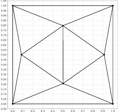
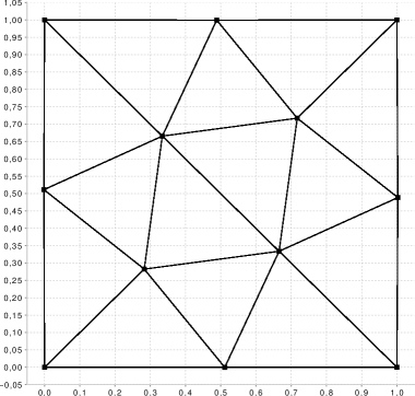
Figure 1: Dual Quantization for $\mathcal{U}([0,1]^{2})$, $N=8$ and $N=12$

​

​

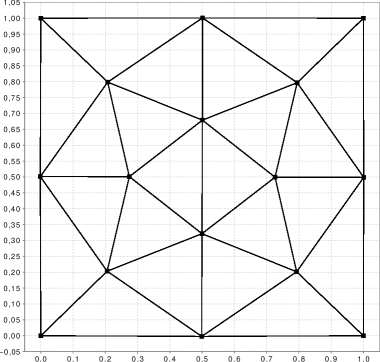
Figure 2: Dual Quantization for $\mathcal{U}([0,1]^{2})$, $N=13$ and $N=16$

​

Figure 3: Dual Quantization for $\mathcal{N}(0,I_{2})$ and $N=250$

​

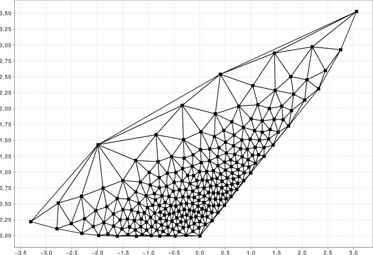
Figure 4: Dual Quantization of the joint distribution a Brownian motion at $T=1$ and its supremum over $[0,1]$ ($N=250$).

Acknowledgement: The authors thank one of the referees for his extremely careful reading of the manuscript.

Appendix

The table below provides in a synthetic way the respective main features of both Voronoi and Delaunay (dual) quantization.

Let $\Gamma=\{x_{1},\ldots,x_{{}_{N}}\}\subset\mathbb{R}^{d}$ be a grid of size $N\geq 1$ and let $F:\mathbb{R}^{d}\to\mathbb{R}$ be a function.

quantization mode	$iq=vq$ (Voronoi)	$iq=dq$ (Delaunay)
		$\widehat{\xi}^{dq}={\cal J}^{*}_{\Gamma}(\omega_{0},\xi)\;$ with $\;{\cal J}^{*}_{\Gamma}(\omega_{0},\xi)=\qquad\qquad$
$\!\!\!\xi\!\in\mathbb{R}^{d}$	$\displaystyle\widehat{\xi}^{vq}=\pi_{\Gamma}(\xi)\!\in\underset{{x_{k}\in\Gamma}}{\rm argmin}\|\xi-x_{k}\|$	$\displaystyle\hskip-5.69046pt\sum_{x_{k}\in{\cal T}(\xi)}\hskip-7.11317ptx_{k}\mbox{\bf 1}_{{}_{\{\lambda^{*}_{1}(\xi)+\cdots+\lambda^{*}_{k-1}(\xi)\leq U(\omega_{0})\leq\lambda^{*}_{1}(\xi)+\cdots+\lambda^{*}_{k}(\xi)\}}}\!\!\in{\cal T}(\xi)\!\subset\Gamma$
$\!\!\!X:\Omega\to\mathbb{R}^{d}$	$\widehat{X}^{vq}=\pi_{{}_{\Gamma}}(X)$	$\widehat{X}^{dq}(\omega_{0},\omega)={\cal J}^{*}_{\Gamma}(\omega_{0},X(\omega))$
$\!\!\!\mathbb{E}\big{(}\widehat{X}^{iq}\,|\,X=\xi\big{)}$	$\widehat{\xi}^{vq}$	$\xi$
$\!\!\!\mathbb{E}\big{(}X|\widehat{X}^{iq}=x_{k}\big{)}$	$x_{k}$ (only if $\Gamma$ is $L^{2}(\mathbb{P}_{{}_{\!X}})$-optimal)	$\times$
$\!\!\!\mathbb{E}\big{(}F(\widehat{X}^{iq})|X=\xi\big{)}$	$F(\widehat{\xi}^{vq})=(F\circ\pi_{\Gamma})(\xi)$	$\displaystyle\mathbb{J}^{*}_{\Gamma}(F)(\xi)\!:=\!\mathbb{E}_{\mathbb{P}_{0}}\big{(}F({\cal J}^{*}_{\Gamma}(\omega_{0},\xi))\big{)}=\sum_{x_{k}\in{\cal T}(\xi)}\lambda^{*}_{k}(\xi)F(x_{k})$
(funct. approx. op.)	(stepwise constant)	(Lipschitz & stepwise affine on $\operatorname{conv}(\Gamma)$)
	$\approx F(\xi)+[F]_{{}_{\rm Lip}}{\rm dist}(\xi,\Gamma)$	$\approx F(\xi)+[DF]_{{}_{\rm Lip}}\mathbb{E}_{\mathbb{P}_{0}}\big{(}\|\widehat{\xi}^{dq}-\xi\|^{2}\big{)}$
$\!\!\!\mathbb{E}\big{(}F(X)|\widehat{X}^{iq}=x_{k}\big{)}$	$\!\approx\!F(x_{k})\!+\![DF]_{{}_{\rm Lip}}\mathbb{E}\big{(}\|X-x_{k}\|^{2}|\widehat{X}^{vq}\!=\!x_{k}\big{)}$
		$\times$
	only if $\Gamma$ is $L^{2}(\mathbb{P}_{{}_{X}})$-optimal

In particular, this table shows that both quantizations methods are connected with a functional approximation operator:

– Voronoi quantization with a projection operator ($F\mapsto F\circ\pi_{\Gamma}$) on stepwise constant functions

– Delaunay quantization with an interpolation operator ($F\mapsto F\circ\mathbb{J}^{*}_{\Gamma}$) on stepwise affine functions.

These two operators are intrinsic in the sense that they do not depend on the distribution of the random vector $X$.

References

- [1] V. Bally and G. Pagès. A quantization algorithm for solving multi-dimensional discrete-time optimal stopping problems. Bernoulli, 9(6):1003–1049, 2003.
- [2] V. Bally, G. Pagès, and J. Printems. A quantization tree method for pricing and hedging multidimensional American options. Mathematical Finance, 15:119–168(50), January 2005.
- [3] O. Bardou, S. Bouthemy, and G Pagès. Optimal Quantization for the Pricing of Swing Options. Applied Mathematical Finance, 16(2):183–217, 2009.
- [4] O. Bardou, S. Bouthemy, and G Pagès. When are Swing options bang-bang? International Journal of Theoretical and Applied Finance (IJTAF), 13(06):867–899, 2010.
- [5] A. L. Bronstein, G. Pagès, and B. Wilbertz. How to speed up the quantization tree algorithm with an application to swing options. Quantitative Finance, 10(9):995–1007, November 2010.
- [6] E. Gobet, G. Pagès, H. Pham, and J. Printems. Discretization and simulation of the Zakai equation. SIAM J. Numer. Anal., 44(6):2505–2538 (electronic), 2006.
- [7] S. Graf and H. Luschgy. Foundations of Quantization for Probability Distributions. Lecture Notes in Mathematics 1730. Springer, Berlin, 2000.
- [8] S. Graf, H. Luschgy, and G. Pagès. Optimal quantizers for Radon random vectors in a Banach space. J. Approx. Theory, 144(1):27–53, 2007.
- [9] M. Padberg. Linear optimization and extensions, volume 12 of Algorithms and Combinatorics. Springer-Verlag, Berlin, expanded edition, 1999.
- [10] G. Pagès, H. Pham, and J. Printems. Optimal quantization methods and applications to numerical methods and applications in finance. In S. Rachev, editor, Handbook of Computational and Numerical Methods in Finance, pages 253–298. Birkhäuser, 2004.
- [11] G. Pagès and J. Printems. Optimal quadratic quantization for numerics: the Gaussian case. Monte Carlo Methods Appl., 9(2):135–166, 2003.
- [12] G. Pagès and B. Wilbertz. Sharp rate for the dual quantization problem. Pre-Print PMA 1402, 2010.
- [13] G. Pagès and B. Wilbertz. Optimal Delaunay and Voronoi quantization schemes for pricing American style options. Pre-Print PMA 1425, to appear in Numerical Methods in Finance, R. Carmona, P. Del Moral, P. Hu, N. Oudjane eds, Springer, 2011.
- [14] H. Pham, W. Runggaldier, and A. Sellami. Approximation by quantization of the filter process and applications to optimal stopping problems under partial observation. Monte Carlo Methods Appl., 11(1):57–81, 2005.
- [15] V. T. Rajan. Optimality of the Delaunay triangulation in . In SCG ’91: Proceedings of the seventh annual symposium on Computational geometry, pages 357–363, New York, NY, USA, 1991. ACM.
- [16] A. Sellami. Comparative survey on nonlinear filtering methods: the quantization and the particle filtering approaches. J. Stat. Comput. Simul., 78(1-2):93–113, 2008.
- [17] A. Sellami. Quantization based filtering method using first order approximation. SIAM J. Numer. Anal., 47(6):4711–4734, 2010.
- [18] B. Wilbertz. Computational aspects of Functional Quantization for Gaussian measures and applications. Diploma Thesis, Trier University, 2005.