Solving Bethe-Salpeter equation for two fermions in Minkowski space

Abstract

The method of solving the Bethe-Salpeter equation in Minkowski space, developed previously for spinless particles bs1 , is extended to a system of two fermions. The method is based on the Nakanishi integral representation of the amplitude and on projecting the equation on the light-front plane. The singularities in the projected two-fermion kernel are regularized without modifying the original BS amplitudes. The numerical solutions for the $J=0$ bound state with the scalar, pseudoscalar and massless vector exchange kernels are found. The stability of the scalar and positronium states without vertex form factor is discussed. Binding energies are in close agreement with the Euclidean results. Corresponding amplitudes in Minkowski space are obtained.

1 Introduction

Bethe-Salpeter (BS) equation for a relativistic bound system was initially formulated in the Minkowski space BS . It determines the binding energy and the BS amplitude. However, in practice, finding the solution in Minkowski space is made difficult due its singular behaviour. The singularities are integrable, but the standard approaches for solving integral equation fail. To circumvent this problem the BS equation is usually transformed, by means of the Wick rotation, into Euclidean momentum space.

The binding energy provided by the Euclidean BS equation is the same than the Minkowski one. For computing the binding energy it is enough to solve the Euclidean BS equation in the rest frame $\vec{p}=0$. While the rest frame solution is not enough to obtain the electromagnetic form factors, since the initial and final states cannot be simultaneously at rest. Contrary to the Minkowski amplitude, the dependence on the total momentum $\vec{p}$ of the Euclidean amplitude is not given by a standard boost, but must be found numerically by solving the Euclidean BS equation for non-zero $\vec{p}$. This requires the rather complicated calculations which were performed in Maris1 ; Maris2 . Within this approach, the hadronic form factors have been calculated, albeit with the aid of additional assumptions.

However, the knowledge of the Euclidean amplitude in a moving system is still not sufficient to calculate some observables, e.g. electromagnetic form factors. The integral providing the form factors contains singularities which are different from those appearing in the BS equation. Their existence invalidates the Wick rotation, to the zero component $k_{0}$, in the form factor integral ckm_ejpa and prevents from obtaining the exact form factors in terms of the Euclidean BS amplitude alone. To avoid this problem, the knowledge of the BS amplitude in Minkowski space is mandatory. Thus, fifty years after its formulation, finding the BS solutions in the Minkowski space is still a field of active research. These solutions would pave the way to numerous applications going from the hadronic electromagnetic form factors of mesons to the deuteron electrodisintegration amplitudes.

Some attempts have been recently made to obtain the Minkowski BS amplitudes. The approach proposed in KW is based on the integral representation of the amplitudes and solutions have been obtained for the ladder scalar case KW ; KW1 ; SA_PRD67_2003 as well as, under some simplifying ansatz, for the fermionic one sauli . Another approach bbmst relies on a separable approximation of the kernel which leads to analytic solutions. Recent applications to the $np$ system can be found in bbpr .

In a previous work bs1 we have proposed a new method to find the BS amplitude in Minkowski space and applied it to the system of two spinless particles.

Our approach consists of two steps. In the first one, the BS amplitude is expressed via the Nakanishi integral representation nakanishi1 ; nakanishi2 :

$$\Phi(k,p) = \int_{-1}^{1}\mbox{d}z^{\prime}\int_{0}^{\infty}\mbox{d}\gamma^{\prime}$$

$$\times \frac{g(\gamma^{\prime},z^{\prime})}{\left[k^{2}+p\cdot k\;z^{\prime}+\frac{1}{4}M^{2}-m^{2}-\gamma^{\prime}+i\epsilon\right]^{3}}.$$

Notice that in this representation, the dependence on the two scalar arguments $k^{2}$ and $p\makebox[2.27626pt]{$\cdot$}k$ of the BS amplitude is made explicit by the integrand denominator and that the weight Nakanishi function $g(\gamma,z)$ is non-singular . By inserting the amplitude (1) into the BS equation on finds an integral equation, still singular, for $g$.

In the second step, we apply to both sides of BS equation an integral transform – light-front projection bs1 – which eliminates singularities of the BS amplitude. It consists in replacing $k\to k+\frac{\omega}{\omega\makebox[2.27626pt]{$\cdot$}p}\,\beta$ where $\omega$ is a light-cone four-vector $\omega^{2}=0$, and integrating over $\beta$ in infinite limits. We obtain in this way, an equation for the non-singular $g(\gamma,z)$. After solving it and substituting the solution in eq. (1), the BS amplitude in Minkowski space can be easily computed.

As a first application we have considered the spinless case with ladder kernel bs1 . The binding energies were compared with the direct solution in the Euclidean space and found to agree each other with high accuracy. By inserting the computed weight function $g$ in (1) and setting $k_{0}=ik_{4}$ the result was found to coincide with the corresponding Euclidean BS amplitude, found independently. The method has been also successfully applied to the cross-ladder kernel bs2 and to compute the electromagnetic form factors ckm_ejpa .

The main difference between our approach and those followed in KW ; KW1 ; SA_PRD67_2003 ; sauli is the use of the light-front projection. This eliminates the singularities related to the BS Minkowski amplitudes. The method is valid for any kernel given by the irreducible Feynman graphs.

We present in this paper the extension of our preceding work bs1 to the two fermion system. In this case the Nakanishi function $g$ is replaced by a set of $n$ functions $g_{i}$, satisfying a system of coupled integral equations, with $n$ depending on the total angular momentum of the state (e.g. $n$=4 for $J=0$, $n$=8 for $J=1$). We will see that the direct application to the fermionic kernels of the method used in the spinless case, is however marred with some numerical difficulties. Although they could be overcome by a proper treatment of the singularities, in this work we propose an alternative method allowing to solve the BS equation for two fermions in Minkowski space with the same degree of accuracy than for the scalar case. The numerical applications will be limited to the $J^{\pi}=0^{+}$ state.

The system of equations for the Nakanishi weight functions $g_{i}$ is derived in sect. 2 starting from the original BS equation. In sect. 3 we develop a regularization procedure for fermionic kernels. Numerical results for the scalar, pseudoscalar and massless vector exchange couplings are presented in sect. 4. Section 5 contains concluding remarks. Some details of the calculations are given in the appendices A, B and C.

2 Derivation of equation

The BS equation for the two fermions vertex function $\Gamma$ reads:

$$\Gamma(k_{1},k_{2},p)C = \int\frac{\mbox{d}^{4}k^{\prime}}{(2\pi)^{4}}iK(k_{1},k_{2},k^{\prime}_{1},k^{\prime}_{2})$$ (2)

$$\times \;\;\Gamma_{1}S(k^{\prime}_{1})\Gamma(k^{\prime}_{1},k^{\prime}_{2},p)CS^{t}(k^{\prime}_{2})\Gamma_{2}^{t}$$ (3)

where $C=\gamma_{2}\gamma_{0}$ is the charge conjugation matrix, $S$ is the fermion propagator

$$S(k^{\prime}_{\alpha})=\frac{i(\hat{k^{\prime}}_{\alpha}+m)}{{k^{\prime}}^{2}_{\alpha}-m^{2}+i\epsilon}\qquad\alpha=1,2$$

$iK$ is the interaction kernel and $\Gamma_{\alpha}$ the fermion-meson vertex. We denote by $\Gamma^{t}_{\alpha}$ its transposed and $\hat{k}=k_{\nu}\gamma^{\nu}$. The charge conjugation matrix $C$ appears here since we construct the vertex function with two fermions in the final state.

We have considered the following fermion ($\Psi,m$) - meson ($\phi,\mu$) interaction Lagrangians:

(i) Scalar coupling

$${\cal L}_{int}^{(s)}=g\,\bar{\Psi}\phi\,\Psi$$ (4)

for which $\Gamma_{\alpha}=ig$

(ii) Pseudoscalar coupling

$${\cal L}_{int}^{(ps)}=ig\,\bar{\Psi}\gamma_{5}\phi\,\Psi$$ (5)

for which $\Gamma_{\alpha}=-g\gamma_{5}$.

(ii) Massless vector exchange

$${\cal L}_{int}^{(v)}=g\,\bar{\Psi}\gamma^{\mu}V^{\mu}\,\Psi$$ (6)

with $\Gamma_{\alpha}=ig\gamma^{\mu}$ and $\Pi_{\mu\nu}=-i{g_{\mu\nu}/q^{2}}$ as vector propagator.

Each interaction vertex has been regularized with a vertex form factor $F(k-k^{\prime})$ by the replacement

$$g\to gF(k-k^{\prime})$$

and we have chosen $F$ in the form:

$$F(q)=\frac{\mu^{2}-\Lambda^{2}}{q^{2}-\Lambda^{2}+i\epsilon}.$$ (7)

The BS amplitude $\Phi$ is defined in terms of the vertex function $\Gamma$ by:

$$\Phi(k_{1},k_{2},p)=S(k_{1})\Gamma(k_{1},k_{2},p)S(-k_{2})$$

Notice that we work with ”unamputated” BS amplitude, which includes the external propagators $S(k_{1}),S(-k_{2})$.

Let us first consider the case of the scalar coupling and the corresponding ladder kernel

$$K=\frac{1}{(k-k^{\prime})^{2}-\mu^{2}+i\epsilon}$$

The BS equation for the amplitude $\Phi$ reads:

$$\Phi(k,p) = \frac{i(m+\frac{1}{2}\hat{p}+\hat{k})}{(\frac{1}{2}p+k)^{2}-m^{2}+i\epsilon}\;\int\frac{\mbox{d}^{4}k^{\prime}}{(2\pi)^{4}}\;\Phi(k^{\prime},p)$$

$$\times \frac{(-ig^{2})\,F^{2}(k-k^{\prime})}{(k-k^{\prime})^{2}-\mu^{2}+i\epsilon}\;\;\frac{i(m-\frac{1}{2}\hat{p}+\hat{k})}{(\frac{1}{2}p-k)^{2}-m^{2}+i\epsilon},$$

where $p=k_{1}+k_{2}$, $k=(k_{1}-k_{2})/2$, $k^{\prime}=(k^{\prime}_{1}-k^{\prime}_{2})/2$.

In the case of $J^{\pi}=0^{+}$ state, the BS amplitude has the following general form:

$$\Phi(k,p)=S_{1}\phi_{1}+S_{2}\phi_{2}+S_{3}\phi_{3}+S_{4}\phi_{4}$$ (9)

where $S_{i}$ are independent spin structures ($4\times 4$ matrices) and $\phi_{i}$ are scalar functions of $k^{2}$ and $p\makebox[2.27626pt]{$\cdot$}k$.

The choice of $S_{i}$ is to some extent arbitrary. To benefit from useful orthogonality properties we have taken

$$S_{1} = \gamma_{5}$$

$$S_{2} = \frac{1}{M}\hat{p}\,\gamma_{5}$$

$$S_{3} = \frac{k\makebox[2.27626pt]{$\cdot$}p}{M^{3}}\hat{p}\,\gamma_{5}-\frac{1}{M}\hat{k}\,\gamma_{5},$$

$$S_{4} = \frac{i}{M^{2}}\sigma_{\mu\nu}p_{\mu}k_{\nu}\,\gamma_{5},$$

where $\sigma_{\mu\nu}=\frac{i}{2}(\gamma_{\mu}\gamma_{\nu}-\gamma_{\nu}\gamma_{\mu})$. The antisymmetry of the amplitude (9) with respect to the permutation $1\leftrightarrow 2$ implies for the scalar functions:

$$\phi_{1,2,4}(k,p) = \phi_{1,2,4}(-k,p)$$ (10)

$$\phi_{3}(k,p) = -\phi_{3}(-k,p)$$ (11)

A decomposition similar to (9) was used in sauli to solve the BS equation for a quark-antiquark system but the solution was approximated keeping only the first term $S_{1}\phi_{1}$.

Substituting (9) in eq. (2), multiplying it by $S_{i}$ and taking traces we get the following system of equations for the invariant functions $\phi_{i}$:

$$\phi_{a}(k,p)=\frac{i}{[(\frac{1}{2}p+k)^{2}-m^{2}+i\epsilon]}\frac{i}{[(\frac{1}{2}p-k)^{2}-m^{2}+i\epsilon]}$$

$$\int\frac{\mbox{d}^{4}k^{\prime}}{(2\pi)^{4}}\frac{(-ig^{2})F^{2}(k-k^{\prime})}{(k-k^{\prime})^{2}-\mu^{2}+i\epsilon}\sum_{a^{\prime}=1}^{4}c_{aa^{\prime}}(k,k^{\prime},p)\phi_{a^{\prime}}(k^{\prime},p)$$ (12)

For scalar and pseudoscalar couplings, the coefficients $c_{ij}$ are given by:

$$c_{ij}=\frac{1}{N_{i}}Tr\left[S_{i}\left(\frac{\hat{p}}{2}+\hat{k}+m\right)\Gamma_{1}S^{\prime}_{j}\bar{\Gamma}_{2}\left(\frac{\hat{p}}{2}-\hat{k}-m\right)\right]$$ (13)

where $N_{i}=Tr[S_{i}^{2}]$ are the normalization factors, $S^{\prime}_{j}$ is obtained from $S_{j}$ by the replacement $k\to k^{\prime}$, $\bar{\Gamma}_{\alpha}=U_{c}\Gamma^{t}_{\alpha}U_{c}=\Gamma_{\alpha}$ with $\Gamma_{\alpha}$ given after eqs. (4) and (5).

For the fermion-fermon vector massless coupling, the $c_{ij}$ coefficients are also given by eq. (13) with the replacement $\Gamma_{1}\to g\gamma_{\nu}$ and $\bar{\Gamma}_{2}\to-g\gamma^{\nu}$ which must be contracted. For the positronium case (fermion-antifermion), they are multiplied by an extra factor $-1$.

The explicit expression of $c_{ij}$ for a $J^{\pi}=0^{+}$ state and the scalar coupling (4) are

$$c_{11} = m^{2}+\frac{1}{4}M^{2}-k^{2}$$

$$c_{12} = mM$$

$$c_{13} = c_{31}=0$$

$$c_{14} = -b^{\prime}M^{2}$$

$$c_{21} = mM$$

$$c_{22} = m^{2}+\frac{1}{4}M^{2}+k^{2}-\frac{2(k\makebox[2.27626pt]{$\cdot$}p)^{2}}{M^{2}}$$

$$c_{23} = -2b^{\prime}(p\makebox[2.27626pt]{$\cdot$}k)$$

$$c_{24} = -2b^{\prime}mM$$

$$c_{32} = 2(p\makebox[2.27626pt]{$\cdot$}k)$$

$$c_{33} = \frac{b^{\prime}}{b}\left(m^{2}-\frac{1}{4}M^{2}+2\frac{(p\makebox[2.27626pt]{$\cdot$}k)^{2}}{M^{2}}-k^{2}\right)$$

$$c_{34} = 2\frac{b^{\prime}}{b}\frac{m}{M}(p\makebox[2.27626pt]{$\cdot$}k)$$

$$c_{41} = M^{2}$$

$$c_{42} = 2mM$$

$$c_{43} = 2\frac{b^{\prime}}{b}\frac{m}{M}(p\makebox[2.27626pt]{$\cdot$}k)$$

$$c_{44} = -\frac{b^{\prime}}{b}\left(\frac{1}{4}M^{2}-m^{2}-k^{2}\right)$$

where

$$b = \frac{1}{M^{4}}\Bigl{[}(p\makebox[2.27626pt]{$\cdot$}k)^{2}-M^{2}k^{2}\Bigr{]}$$

$$b^{\prime} = \frac{1}{M^{4}}\Bigl{[}(p\makebox[2.27626pt]{$\cdot$}k)(p\makebox[2.27626pt]{$\cdot$}k^{\prime})-M^{2}(k\makebox[2.27626pt]{$\cdot$}k^{\prime})\Bigr{]}$$

The coefficients $c_{ij}$ for the pseudoscalar exchange (5) are simply obtained by changing the sign of the $j=1$ and $j=4$ matrix elements in the scalar ones:

$$c^{PS}_{ij=1,4}=-c^{S}_{ij=1,4}\qquad,\forall i$$ (14)

For the massless vector exchange (6) the coefficients are given by

$$c^{V}_{ij}=\xi_{ij}\;c^{S}_{ij},\qquad\xi=\pmatrix{4&-2&0&0\cr 4&-2&-2&0\cr 0&-2&-2&0\cr 4&-2&-2&0}$$ (15)

The equation (2) is the Minkowski space BS equation for two fermions we aim to solve. As in the scalar case, the BS amplitudes $\phi_{i}$ are singular and a direct solution of (2) is not suitable even for the simplest kernels.

To overcome this difficulty, the first idea is to represent each of the BS components $\phi_{i}(k,p)$ by means of the Nakanishi integral

$$\phi_{i}(k,p) = \int_{-1}^{1}\mbox{d}z^{\prime}\int_{0}^{\infty}\mbox{d}\gamma^{\prime}$$

$$\times \frac{g_{i}(\gamma^{\prime},z^{\prime})}{\left[k^{2}+p\cdot k\;z^{\prime}+\frac{1}{4}M^{2}-m^{2}-\gamma^{\prime}+i\epsilon\right]^{3}}.$$

and apply the light-front projection to the set of coupled equations for the corresponding weight functions $g_{i}(\gamma,z)$. As mentioned in the Introduction, this projection, which is an essential ingredient of our previous works bs1 ; bs2 , consists in replacing $k\to k+{\omega\over\omega\cdot p}\beta$ in eq. (2) and integrating over $\beta$ in all the real domain. This integration is quite similar to the case of the spinless particles explained in detail in bs1 .

We obtain in this way a set of coupled two-dimensional integral equations which can be written in the general form valid for all types of couplings and states:

$$\int_{0}^{\infty}\mbox{d}\gamma^{\prime}\frac{1}{\left[D_{0}(\gamma,z)+\gamma^{\prime}\right]^{2}}\;g_{i}(\gamma^{\prime},z)=$$ (17)

$$\sum_{j}\int_{0}^{\infty}\mbox{d}\gamma^{\prime}\int_{-1}^{+1}\mbox{d}z^{\prime}\;V_{ij}(\gamma,z,\gamma^{\prime},z^{\prime})\;g_{j}(\gamma^{\prime},z^{\prime})$$ (18)

where

$$D_{0}(\gamma,z)=\gamma+m^{2}z^{2}+(1-z^{2})\kappa^{2}$$

and

$$\kappa^{2}=m^{2}-{M^{2}\over 4}$$

The left hand side of (17) is the same for all the amplitudes and coincides with the scalar case bs1 .

The interaction kernel $V_{ij}$ can be written in the form

$$V_{ij}(\gamma,z,\gamma^{\prime},z^{\prime})=\left\{\begin{array}[]{rl}W_{ij}(\gamma,z,\gamma^{\prime},z^{\prime})&{\rm if}\ z^{\prime}\leq z\\ \sigma_{ij}\;W_{ij}(\gamma,-z,\gamma^{\prime},-z^{\prime})&{\rm if}\ z^{\prime}>z\end{array}\right.$$ (19)

with

$$\sigma=\pmatrix{+1&+1&-1&+1\cr+1&+1&-1&+1\cr-1&-1&+1&-1\cr+1&+1&-1&+1}$$ (20)

and

$$W_{ij}(\gamma,z,\gamma^{\prime},z^{\prime})={\alpha m^{2}\over 2\pi}\frac{(1-z)^{2}}{D_{0}}$$ (21)

$$\int_{0}^{1}Z_{\Lambda}(\gamma,z,\gamma^{\prime},z^{\prime};v)\;C_{ij}(\gamma,z;v)\;{v^{2}\over D^{2}}\mbox{d}v$$ (22)

We use here $\alpha={g^{2}\over 4\pi}$, whereas the denominator

$$D(\gamma,z,\gamma^{\prime},z^{\prime},v) = v(1-v)(1-z^{\prime})\gamma$$

$$+ vm^{2}\;[(1-v)(1-z^{\prime})z^{2}+v{z^{\prime}}^{2}(1-z)\;]$$

$$+ v\kappa^{2}(1-z)(1-z^{\prime})\;[1+z-v(z-z^{\prime})\;]$$

$$+ (1-z)[(1-v)\mu^{2}+v\gamma^{\prime}]$$

is the same than in our previous work bs1 .

The function

$$Z_{\Lambda} = (1-v)^{2}(1-z)^{2}$$

$$\times \frac{\left[3D+(1-v)(1-z)(\Lambda^{2}-\mu^{2})\right](\Lambda^{2}-\mu^{2})^{2}}{[D+(1-v)(1-z)(\Lambda^{2}-\mu^{2})]^{3}}$$

contains the dependence on the vertex form factor parameter $\Lambda$ with

$$\lim_{\Lambda\to\infty}Z_{\Lambda}=1$$

The matrix coefficients $C_{ij}$ couple the different spin components. They are given in appendix A for the $J^{\pi}=0^{+}$ states. Notice that setting $C_{ij}=\delta_{ij}$ and $Z_{\Lambda}=1$ the set of eqs. (17) decouples and each of them is identical to the spinless case one given in bs1 .

It turns out that, in contrast to the scalar case, most of the kernel matrix elements $V_{ij}$ are discontinuous at $z^{\prime}=z$. In some cases – like e.g. $V_{14}$ displayed in fig. 1 – the value of the discontinuity, although being finite at fixed value of $z$, diverges when $z\to\pm 1$. This creates some numerical difficulties when computing the solutions $g_{i}(\gamma,z)$ in the vicinity of $z=\pm 1$. They can be in principle solved by properly taking into account the particular type of divergence. However the latter may depend on the particular matrix element, on the type of coupling, the quantum number of the state and other details of the calculation. We propose in next section an alternative, and efficient way to overcome this difficulty.

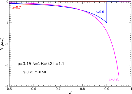
Figure 1: The kernel matrix element $V_{14}(\gamma,z;\gamma^{\prime},z^{\prime})$, eq. (19), for $z=0.7,0.9,0.95$ as a function of $z^{\prime}$ and fixed values of $\gamma,\gamma^{\prime}$. The discontinuity is finite at a fixed value of $z$ but diverges when $z\to 1$.

3 Regularized kernels

To deal with more regular kernels, the original BS equation (2) is first multiplied on both sides of by the factor

$$\eta(k,p)=\frac{(m^{2}-L^{2})}{\left[(\frac{p}{2}+k)^{2}-L^{2}+i\epsilon\right]}\frac{(m^{2}-L^{2})}{\left[(\frac{p}{2}-k)^{2}-L^{2}+i\epsilon\right]}$$ (23)

This factor has the form of a product of two scalar propagators with mass $L$. It plays the role of form factor suppressing the high off-mass shell values of the constituent four-momenta $k^{2}_{1,2}=(\frac{p}{2}\pm k)^{2}$ and tends to 1 when $L\to\infty$.

The light-front projection and Nakanishi transform are then applied to the equation

$$\eta(k,p)\;\phi_{i}(k,p)=$$

$$\frac{\eta(k,p)}{[(\frac{p}{2}+k)^{2}-m^{2}+i\epsilon][(\frac{p}{2}-k)^{2}-m^{2}+i\epsilon]}$$

$$\times \int\frac{\mbox{d}^{4}k^{\prime}}{(2\pi)^{4}}\frac{ig^{2}\,F^{2}(k-k^{\prime})}{(k-k^{\prime})^{2}-\mu^{2}+i\epsilon}\sum_{j=1}^{4}c_{ij}(k,k^{\prime},p)\phi_{j}(k^{\prime},p),$$

Since $\eta(k,p)\neq 0$, the equation thus obtained is strictly equivalent to (2). We will see however that, due to the presence of the $\eta$ factor, the light front projection modifies the resulting kernels which become less singular functions.

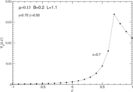
Figure 2: The left hand side kernel $V^{g}(\gamma=0.75,z=0.7,\gamma=0.5,z^{\prime})$, eq. (26), as a function of $z^{\prime}$ for L=1.1 m

The technical details of the light-front projection are similar to those given in ref. bs1 . The differences, due to the factor $\eta(k,p)$, are explained in Appendix B. The new set of equations has the following form:

$$\int_{0}^{\infty}\mbox{d}\gamma^{\prime}\int_{-1}^{1}\mbox{d}z^{\prime}\;V^{g}(\gamma,z;\gamma^{\prime},z^{\prime})\;g_{i}(\gamma^{\prime},z^{\prime})=$$

$$\sum_{j}\int_{0}^{\infty}\mbox{d}\gamma^{\prime}\int_{-1}^{1}\mbox{d}z^{\prime}\;V^{d}_{ij}(\gamma,z;\gamma^{\prime},z^{\prime})g_{j}(\gamma^{\prime},z^{\prime})$$ (25)

The kernels $V^{g}$ and $V^{d}_{ij}$ depend now on the parameter $L$. Closer is $L$ to $m$, smoother is the kernel and more stable are the numerical solutions. However the weight functions $g_{i}(\gamma,z)$ as well as binding energies provided by (3) are independent of $L$.

Notice that, in contrast to (17), the left hand side of eq. (3) is also a two-dimensional integral. The corresponding kernel $V^{g}$ is the same for all the components and has the form:

$$V^{g}(\gamma,z;\gamma^{\prime},z^{\prime})=\left\{\begin{array}[]{ll}W^{g}(\gamma,z;\gamma^{\prime},z^{\prime})&\;\;\mbox{if $z^{\prime}\leq z$}\\ W^{g}(\gamma,-z;\gamma^{\prime},-z^{\prime})&\;\;\mbox{if $z^{\prime}>z$}\end{array}\right.$$ (26)

with

$$W^{g}(\gamma,z;\gamma^{\prime},z^{\prime})=\frac{(L^{2}-m^{2})}{H^{3}}$$ (27)

and

$$H = \gamma\frac{(1-z^{\prime})}{(1-z)}+\gamma^{\prime}+(1-z^{\prime})(1+z)\kappa^{2}$$

$$+ \Bigl{(}z^{\prime}-z(1-z^{\prime})\Bigr{)}m^{2}+\frac{(z-z^{\prime})}{(1-z)}L^{2}$$

To avoid spurious singularities in (27) due to the $\eta$ factor (23), $L^{2}$ must be larger than $\frac{M^{2}}{2}-m^{2}$, what is fulfilled for $L>m$. In practical calculations we have taken $m=1$ and $L=1.1$.

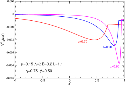
Figure 3: Regularized right hand side kernel $V^{d}_{14}(\gamma,z;\gamma^{\prime},z^{\prime})$, eq. (28), v.s. fixed values of $z=0.7,\;0.9,\;0.95$ and $L=1.1\,m$. Compare with fig. 1.

The kernel $V_{g}$ is finite and vanishes for $z=\pm 1$. For a fixed values of $\gamma,z$ and $\gamma^{\prime}$, $V_{g}$ is a continuous function of $z^{\prime}$ with a discontinuous derivative at $z^{\prime}=z$. It is represented in fig. 2 for $z=0.7$.

The right hand side kernel $V^{d}_{ij}$ is given by:

$$V^{d}_{ij}(\gamma,z;\gamma^{\prime},z^{\prime})=\left\{\begin{array}[]{ll}\phantom{\sigma_{ij}}W^{d}_{ij}(\gamma,z;\gamma^{\prime},z^{\prime})&\;\mbox{if $z^{\prime}<z$}\\ \sigma_{ij}W^{d}_{ij}(\gamma,-z;\gamma^{\prime},-z^{\prime})&\;\mbox{if $z^{\prime}>z$}\end{array}\right.$$ (28)

$W^{d}_{ij}$ is represented as a sum of two terms:

$$W^{d}_{ij}=W^{a}_{ij}+W^{b}_{ij}$$

which can be written in the same form than (21)

$$W^{\nu}_{ij}(\gamma,z,\gamma^{\prime},z^{\prime})={\alpha m^{2}\over 2\pi}\frac{(1-z)^{2}}{D_{0}}F^{\nu}_{L}(\gamma,z)$$ (29)

$$\times\int_{0}^{1}Z^{\nu}_{\Lambda}(\gamma,z,\gamma^{\prime},z^{\prime};v)\;C^{\nu}_{ij}(\gamma,z;v)\;{v^{2}\over D_{\nu}^{2}}\mbox{d}v$$ (30)

For the first term ($\nu=a$) one has

$$F^{a}_{L} = \frac{(1-z)\;[D_{0}+(L^{2}-m^{2})]}{2D_{0}+(1-z)(L^{2}-m^{2})}$$

$$Z^{a}_{\Lambda} = Z_{\Lambda}$$

$$C^{a}_{ij} = C_{ij}$$

$$D_{a} = D$$

where $Z_{\Lambda},C_{ij}$ and $D$ are the same than in eq. (21).

For the second term ($\nu=b$) one has

$$F^{b}_{L} = -\frac{D_{0}(1-z)}{2D_{0}+(1+z)(L^{2}-m^{2})}$$

$$Z^{b}_{\Lambda} = (1-v)^{2}(1-z)^{2}$$

$$\times \frac{\left[3D_{b}+(1-v)(1-z)(\Lambda^{2}-\mu^{2})\right](\Lambda^{2}-\mu^{2})^{2}}{[D_{b}+(1-v)(1-z)(\Lambda^{2}-\mu^{2})]^{3}}$$

$$D_{b} = D_{a}+v(1-v)(z-z^{\prime})(L^{2}-m^{2})$$

with the coefficients $C^{b}_{ij}$ given in Appendix C.

Notice that, like $Z_{\Lambda}$, $Z^{b}_{\Lambda}\to 1$ when $\Lambda\to\infty$. Notice also that $F^{a}_{L}\to 1$ and $F^{b}_{L}\to 0$ in the limit $L\to\infty$. One has consequently $W^{a}=W$, $W^{b}=0$ and $V^{d}=V$ given in (19). Furthermore the peak at $z^{\prime}=z$ in the left kernel $V^{g}$ displayed in fig. 2 tends to a delta function $\delta(z^{\prime}-z)$ with a coefficient which reproduces the left-hand side of eq. (17).

For a finite value of $L$, both systems of equations are also strictly equivalent to each other but the $z^{\prime}$-dependence of the regularized kernels is much more smooth and therefore better adapted for obtaining accurate numerical solutions. In fig. 3 we plotted the regularized kernel $V^{d}_{14}$ as a function of $z^{\prime}$ for the same arguments $\gamma,z,\gamma^{\prime}$ and parameters than in fig. 1, where it was calculated without the $\eta(k,p)$ factor. As one can see, the kernel is now a continuous function of $z^{\prime}$. A discontinuity of the first derivative however remains at $z^{\prime}=z$.

Some additional remarks concerning the regularization procedure presented in this section are in order:

(i) The most singular kernel is $V_{23}$. It is the only matrix element that after regularization by means of the $\eta(k,p)$ factor remains discontinuous at $z^{\prime}=z$ . The degree of the discontinuity in the limit $z\to\pm 1$ is however reduced and does no longer spoil the numerical accuracy.

(ii) This procedure can be improved by choosing for $\eta(k,p)$ a more strongly decreasing function of the arguments $\left(\frac{p}{2}\pm k\right)^{2}$. The simple replacement $\eta(L)\to\eta(L_{1})\eta(L_{2})$ would reduce the degree of singularity of the remaining singular matrix elements in the limit $z\to\pm 1$. We have not found any need for that in the present calculations.

(iii) We would like to emphasize again that despite the fact that the non-regularized and regularized kernels are very different from each other (compare e.g. the figs. 1 and 3) and that the regularized ones strongly depends on the value of $L$, they provide – up to numerical errors – the same binding energies and weight functions $g_{i}(\gamma,z)$. We construct in this way a family of equivalent kernels.

Table 1: Coupling constant $g^{2}$ as a function of binding energy $B$ for the $J=0$ state with scalar (S), pseudoscalar (PS) and massless vector (positronium) exchange kernels. The vertex form factor is $\Lambda=2$ and the parameter of the $\eta$ factor $L=1.1$.

	S		PS		positronium
$\mu$	0.15	0.50	0.15	0.50	0.0
$B$	$g^{2}$	$g^{2}$	$g^{2}$	$g^{2}$	$g^{2}$
0.01	7.813	25.23	224.8	422.3	3.265
0.02	10.05	29.49	232.9	430.1	4.910
0.03	11.95	33.01	238.5	435.8	6.263
0.04	13.69	36.19	243.1	440.4	7.457
0.05	15.35	39.19	247.0	444.3	8.548
0.10	23.12	52.82	262.1	459.9	13.15
0.20	38.32	78.25	282.9	480.7	20.43
0.30	54.20	103.8	298.6	497.4	26.50
0.40	71.07	130.7	311.8	515.2	31.84
0.50	86.95	157.4	323.1	525.9	36.62

4 Numerical results

The solutions of eq. (3) have been obtained using the same techniques than in ref bs1 , i. e. spline expansion of the Nakanishi weight functions

$$g_{i}(\gamma,z)=\sum_{\alpha\beta}g_{i,\alpha\beta}S_{\alpha}(\gamma)S_{\beta}(z)$$

on a compact domain $\Omega=[0,\gamma_{max}]\times[-1,+1]$ and validation of the equations in some well chosen points in the $N_{\gamma}\times N_{z}$ corresponding intervals. The unknown coefficients $g_{i,\alpha\beta}$ and the total mass $M$ are obtained by solving a generalized eigenvalue problem

$$\lambda N(M)g=A(M)g$$

As in the scalar case, the discretized left hand side kernel $N$ has very small eigenvalues which make difficult the solution using standard methods. This is avoided by adding a small constant term of the form

$$N=N+\epsilon_{R}I$$

where $I$ is the identity operator in the spline basis. The error in the eigenvalues thus induced is of the order of $\epsilon_{R}$ and we have taken $\epsilon_{R}=10^{-6}$.

We have computed the binding energies, defined as $B=2m-M$, and BS amplitudes, for the $J=0^{+}$ two fermion system interacting with massive scalar (S) and pseudoscalar (PS) exchange kernels and for the fermion-antifermion system interacting with massless vector exchange in Feynman gauge. In the limit of an infinite vertex form factor parameter $\Lambda\to\infty$, the later case would correspond to positronium with an arbitrary value of the coupling constant. All the results presented in this section are given in the constituent mass units ($m=1$) and with $L=1.1$.

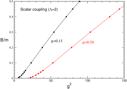
Figure 4: Binding energy for scalar exchange v.s. $g^{2}$ for $\Lambda=2$, $L=1.1$, $\mu=0.15$ and $\mu=0.5$.

The binding energies obtained with the form factor parameter $\Lambda=2$ are given in table 1. For the scalar and pseudoscalar cases, we present the results for $\mu=0.15$ and $\mu=0.50$ boson masses. They have been compared to those obtained in a previous calculation in Euclidean space dorkin ; Dorkin_PC using a slightly different form factor. Notice, that contrary to what is written in eq. (16) of dorkin – which coincides with our form factor (7) – the vertex form factor used in these calculations is Dorkin_PC

$$F(q^{2})={\Lambda^{2}\over\Lambda^{2}-q^{2}+i\epsilon}$$

Once taken into account this correction, our scalar results are in full agreement (four digits) with dorkin ; Dorkin_PC . The pseudoscalar ones show small discrepancies ($\approx 0.5\%$). We have also computed CK_Euc the binding energies by directly solving the fermion BS equation the Euclidean space using a method independent of the one used in dorkin . Our Euclidean results are in full agreement with those given in the table 1.

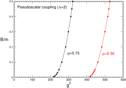
Figure 5: Binding energy for pseudoscalar exchange v.s. $g^{2}$ for $\Lambda=2$, $L=1.1$, $\mu=0.15$ and $\mu=0.5$.

The $B(g^{2})$ dependence for the scalar and pseudoscalar couplings is plotted in figs. 4 and 5. Notice the different $g^{2}$ scales of both dependences. The pseudoscalar binding energies are fast increasing functions of $g^{2}$ and thus more sensitive to the accuracy of numerical methods. This sharp behaviour was also exhibit when solving the corresponding Light-Front equation MCK_PRC68_2003 .

It is worth noticing that the stability properties of the BS $J^{\pi}=0^{+}$ solutions for the scalar coupling are very similar to the Light-Front ones. In the latter case, we have shown MCK_PRD64RC_2003 ; MCK_PRD64_2003 the existence of a critical coupling constant $g_{c}$ below which the system is stable without vertex form factor while for $g>g_{c}$, the system ”collapses”, i.e. the spectrum is unbounded from below. The numerical value was found to be $\alpha_{c}=3.72$ MCK_PRD64_2003 , which corresponds to $g_{c}=6.84$. Performing the same analysis than in our previous work – eq. (71) from MCK_PRD64_2003 – we found that for BS equation the critical coupling constant is $g_{c}=2\pi$, in agreement with dorkin . The $10\%$ difference between the numerical values of $g_{c}$ is apparently due to the different contents of the intermediate states in the two approaches. The ladder BS equation incorporates effectively the so-called stretch-boxes diagrams which are not taken into account in the ladder LF results.

The positronium case deserves some comments. First we would like to notice that in our formalism, the singularity of the Coulomb-like kernels in terms of the momentum transfer $1/(k-k^{\prime})^{2}$ is absent. This is a combined consequence of the Nakanishi transform (1) – which allows to integrate over $k^{\prime}$ analytically in the right hand side of the BS equation (2) – and of the consecutive light front projection integral. After this integration, the Coulomb singularity does not anymore manifest itself in the kernel. This can be explicitly seen in the kernel of the Wick-Cutkosky model obtained in eq. (22) of our previous work bs1 .

A second remark concerns the $\Lambda$ dependence of the positronium results. Using the methods developed in MCK_PRD64RC_2003 ; MCK_PRD64_2003 we found that in the BS approach with ladder kernel there also exists a critical value of the coupling constant $g_{c}=\pi$. Note that, as in the scalar coupling, the very existence and the value of this critical coupling constant is independent on the constituent ($m$) and exchange $\mu$ masses but depends on the quantum number of the state.

Table 2: Coupling constant $g^{2}$ as a function of binding energy $B$ for the positronium $J=0$ state in BS equation in the region of stability without vertex form factor ($\Lambda\to\infty$), i.e. $g<\pi$. They are compared to the non relativistic results.

$B$	$g^{2}_{NR}$	$g^{2}_{BS}$
0.01	2.51	3.18
0.02	3.55	4.65
0.03	4.35	5.75
0.04	5.03	6.64
0.05	5.62	7.38
0.06	7.95	8.02
0.07	11.24	8.57
0.08	13.77	9.06
0.09	15.90	9.49

The ground state positronium binding energies without vertex form factor are given in table 2 for values of the coupling below $g_{c}$, Nonrelativistic results

$$g^{2}_{NR}=8\pi\sqrt{B/m}$$

are included for comparison. One can see that the relativistic effects are repulsive.

These results are displayed in fig. 6 (black solid line), and compared to the binding energies obtained with two values of the form factor parameter $\Lambda=2$ (dashed) and $\Lambda=5$ (dot-dashed). The stability region is limited by a vertical dotted line at $g=g_{c}=\pi$. Beyond this value the binding energy without form factor becomes infinite and we have found $B(g\to g_{c})\approx 0.10$.

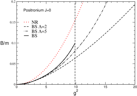
Figure 6: Binding energy for $J=0$ positronium state versus $g^{2}$ (black solid line) in the stability region $g<g_{c}=\pi$. Dashed and dotted-dashed curves correspond to the results for increasing values of the vertex form factor parameter $\Lambda=2$ and $\Lambda=5$ respectively. They are compared to the non relativistic results (dotted line).

The inclusion of the form form factor has a repulsive effect, i.e. for a fixed value of the coupling constant it provides a binding energy of the system which is smaller than in the $\Lambda\to\infty$ limit (no cut-off). This is also illustrated in fig. 7 where we have plotted the $\Lambda$ dependence of $g^{2}$ for two different energies. One can see that the value of the coupling constant to produce a bound state is a decreasing function of $\Lambda$. The size of the effect depends strongly on the binding energy but for both energies the asymptotics is reached at $\Lambda\approx 20$. This behaviour is understandable in terms of regularizing the short range singularity of $-1/r^{2}$ interactions.

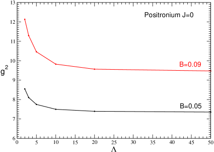
Figure 7: $\Lambda$-dependence of $g^{2}$ for $J=0$ positronium state for fixed values of binding energies $B=0.05$ and $B=0.09$.

Finally we present some examples of the Nakanishi weigh functions $g_{i}(\gamma,z)$. They correspond to a $B=0.1$ state with the scalar coupling and the same parameters $\Lambda=2$, $\mu=0.50$ than in table 1. They are displayed in fig. 8. In the upper figure is shown the $\gamma$-dependence for a fixed value of $z$ and in the lower figure the $z$-dependence for a fixed $\gamma$. Notice the regular behaviour of these functions as well as their well defined parity with respect to $z$ – $g_{1,2,4}$ are even and $g_{3}$ is odd – consequence of relations (11) . As in the scalar case the $\epsilon_{R}$-dependence of $g_{i}$ is more important than for the binding energy.

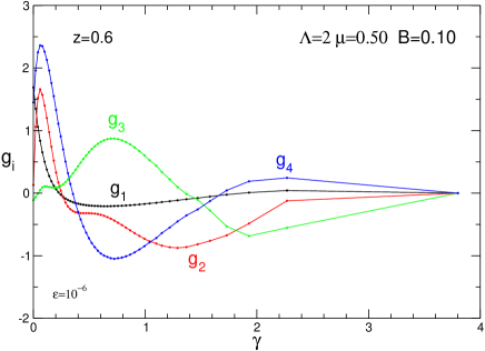
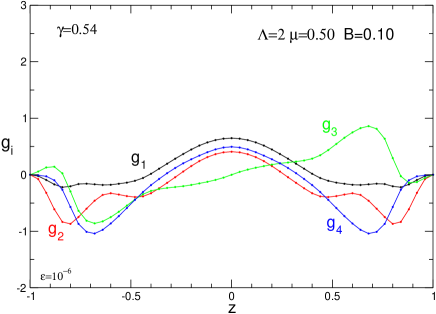
Figure 8: Nakanishi weight functions for scalar exchange for $\Lambda=2$, $B=0.10$, $\mu=0.50$ and $L=1.1$.

Corresponding BS amplitudes $\phi_{i}$ are displayed in fig. 9. Their computation by directly applying equation (2) is not very suitable due to the zeroes of the integrand denominator. We have preferred to compute $\phi_{i}$ by first factorizing the pole singularities in the right hand side of eq. (2)

$$\phi_{a}(k,p)=\frac{i^{2}\tilde{\Gamma}_{a}(k,p)}{{[(\frac{1}{2}p+k)^{2}-m^{2}+i\epsilon]}{[(\frac{1}{2}p-k)^{2}-m^{2}+i\epsilon]}}$$

and computing $\tilde{\Gamma}_{a}$ which is a regular function of $k$. By inserting the Nakanishi transform (2) in the expression for $\tilde{\Gamma}_{a}$, the integral over $k^{\prime}$ in (2) can be performed analytically and obtains the form

$${\tilde{\Gamma}_{a}}(k,p)=\sum_{a^{\prime}}\int_{0}^{\infty}\mbox{d}\gamma\int_{-1}^{+1}\mbox{d}z\;I_{aa^{\prime}}(k,p,\gamma,z)g_{a^{\prime}}(\gamma,z)$$

where $I_{aa^{\prime}}$ is a more appropriate function for computation purposes.

The upper figure 9 represents the $k_{0}$ dependence of $\phi_{i}$ for a fixed value of $\mid\vec{k}\mid=0.2$. They exhibit a singular behaviour which corresponds to the pole of free propagators $k_{0}=\epsilon_{k}-{M\over 2}$. The lower figure represents the $\mid\vec{k}\mid$ dependence of the amplitudes $\phi_{i}$ for a fixed value $k_{0}=0.04$. For this choice of arguments, the amplitudes are smooth functions of $\mid\vec{k}\mid$, though they will be also singular for $k_{0}>{B\over 2}=0.05$. Notice that all the infinities in the BS amplitudes $\phi_{i}$ come from the free propagator. However $\tilde{\Gamma}_{a}$, although being smooth, has its own non-analytical points. For instance it obtains an imaginary part for $({p\over 2}\pm k)^{2}>(m+\mu)^{2}$ .

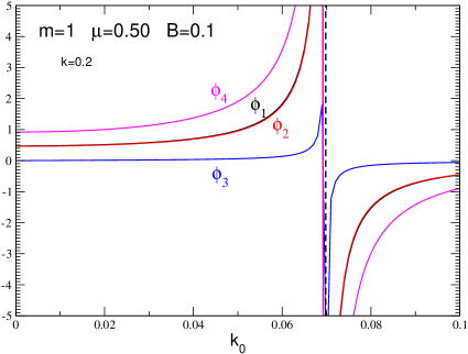
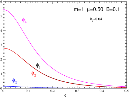
Figure 9: Bethe-Salpeter Minkowski amplitudes corresponding to fig. 8. Here $k=\mid\vec{k}\mid$. The amplitudes $\phi_{1}$ and $\phi_{2}$ are indistinguishable.

5 Conclusions

We present a new method for obtaining the solutions of the Bethe-Salpeter equation in Minkowski space for the two-fermion system. It is based on a Nakanishi integral representation of the amplitude and Light-Front projection and constitutes a natural extension our previous work for the scalar case bs1 .

A straightforward generalization of this approach, however results into a singular fermionic kernel. In order to smooth this singularities, a proper regularization of the kernels has been proposed. This generates a family of strictly equivalent equations depending on one parameter $L$. Their solution gives the same binding energies and Nakanishi weight functions $g_{i}(\gamma,z)$ .

The binding energies for the scalar and pseudoscalar exchange kernels and for massless vector exchange (positronium) are found. They coincide with the ones found via Euclidean space solution, thus providing a validity test of our method. The solutions for the scalar and positronium states without vertex form factor ($\Lambda\to\infty$) are found to be stable below some critical value $g_{c}$ of the coupling constant, respectively $g_{c}=2\pi$ (scalar) and $g_{c}=\pi$ (positronium).

The BS amplitudes are obtained in terms of the computed Nakanishi weight functions. The exhibit a singular behaviour due, on one hand, to the poles of the free propagators and, on the other hand, to non analytic branch cuts which are responsible for the appearance of an imaginary part.

An alternative approach to avoid the singularities of the Minkowski amplitude would be to solve the BS equation in the Euclidean space in terms of the Nakanishi weight functions. Once solved, we can again restore the Minkowski BS amplitude by the integral (1). These different methods should provide the same solutions although with different precision and stability. The results of this study will be published in a future paper CK_Euc .

Appendix A The coefficients $C_{ij}$

The spin-coupling matrix elements $C_{ij}(\gamma,z;v)$ in eq. (21) determining the kernel of the equation (17), and also the kernel (29) at $\nu=a$, for the $J=0$ state and scalar coupling are:

$$\begin{array}[]{lcl}C_{11}&=&\frac{1}{(1-z)}\;\frac{Q_{+}}{4m^{2}}\\ C_{12}&=&\frac{M}{4m}\\ C_{13}&=&0\\ C_{14}&=&-{(1-v)\over(1-z)^{2}}\;{K_{+}\;K_{-}\over 4m^{2}M^{2}}\\ C_{21}&=&C_{12}\\ C_{22}&=&-\frac{(\gamma+m^{2})^{2}}{(1-z)^{2}2m^{2}M^{2}}+\frac{\gamma z+(2-z)m^{2}}{4m^{2}(1-z)}+\frac{(1-z^{2})M^{2}}{32m^{2}}\\ C_{23}&=&-\frac{1-v}{(1-z)^{3}}\;{K_{+}\;K_{-}\;Q_{-}\over 2m^{2}M^{4}}\\ C_{24}&=&-{1-v\over(1-z)^{2}}\;{K_{+}\;K_{-}\over 2mM^{3}}\\ C_{31}&=&0\\ C_{32}&=&{1\over(1-z)}\;\frac{Q_{-}}{2m^{2}}\\ C_{33}&=&{1-v\over(1-z)^{2}}\;{Q_{-}\;Q_{+}\over 2m^{2}M^{2}}\\ C_{34}&=&{1-v\over 1-z}\;\frac{Q_{-}}{2mM}\\ C_{41}&=&\frac{M^{2}}{4m^{2}}\\ C_{42}&=&2\;C_{12}\\ C_{43}&=&C_{34}\\ C_{44}&=&-{1-v\over 1-z}\frac{4\gamma-4(1-2z)m^{2}+(1-z)^{2}M^{2}}{16m^{2}}\end{array}$$

with

$$K_{\pm} = \gamma+\left(m\pm{M\over 2}(1-z)\right)^{2}$$

$$Q_{\pm} = \gamma+m^{2}\pm{M^{2}\over 4}(1-z)^{2}$$

The coefficients for the pseudoscalar and massless vector exchange are given by the relations (14) and (15) respectively.

Appendix B Derivation of the equation (3)

In order to derive the equation (3), we substitute in eq. (3) the amplitudes $\phi_{i}(k,p)$ in the form (1), shift the variable $k\to k+\frac{\omega}{\omega\makebox[2.27626pt]{$\cdot$}p}\beta$ and integrate over $\beta$ in the infinite limits.

The integrand depends on the scalar variables $k^{2},\;p\makebox[2.27626pt]{$\cdot$}k$ and $\frac{\omega\makebox[2.27626pt]{$\cdot$}k}{\omega\makebox[2.27626pt]{$\cdot$}p}$ which are not independent but are related to each other by a constrain. Following appendix A from bs1 , we parametrize them in terms of two independent variables $\gamma,z$ as:

$$k^{2} = -\frac{(\gamma+z^{2}m^{2})}{1-z^{2}}$$

$$\frac{\omega\makebox[2.27626pt]{$\cdot$}k}{\omega\makebox[2.27626pt]{$\cdot$}p} = -\frac{1}{2}z$$

$$p\makebox[2.27626pt]{$\cdot$}k = \frac{z[\gamma+z^{2}m^{2}+(1-z^{2})\kappa^{2}]}{1-z^{2}},$$

where $\kappa^{2}=m^{2}-\frac{1}{4}M^{2}$. In the spinless case bs1 , when we applied integration over $\beta$ to the equation without the factor $\eta(k,p)$, we found that its left-hand side obtained the form:

$$l.h.s.=\int_{-1}^{1}\mbox{d}z^{\prime}\int_{0}^{\infty}\mbox{d}\gamma^{\prime}\int_{-\infty}^{\infty}d\beta$$ (31)

$$\times\frac{g(\gamma^{\prime},z^{\prime})}{\left[\beta(z-z^{\prime})+\gamma^{\prime}+(1-zz^{\prime})\left(\kappa^{2}+\frac{\gamma+m^{2}z^{2}}{1-z^{2}}\right)-i\epsilon\right]^{3}}$$

As a function of $\beta$, it contains one pole at

$$\beta^{\prime}_{0}=\frac{+i\epsilon}{z-z^{\prime}}.$$ (32)

Taking the residue, we found that the result of integration is proportional to $\delta(z^{\prime}-z)$ and consequently the left-hand side obtained the form of a one-dimensional integral:

$$l.h.s.=\int_{0}^{\infty}\frac{i\pi\,g(\gamma^{\prime},z)\mbox{d}\gamma^{\prime}}{\Bigl{[}\gamma^{\prime}+\gamma+z^{2}m^{2}+(1-z^{2})\kappa^{2}\Bigr{]}^{2}}$$

The factor $\eta(k,p)$ itself consists of two factors. Therefore, after replacement $k\to k+\frac{\omega}{\omega\makebox[2.27626pt]{$\cdot$}p}\,\beta$, the factor $\eta(k+\frac{\omega}{\omega\makebox[2.27626pt]{$\cdot$}p}\beta,p)$ v.s. $\beta$ obtains two poles:

$$\beta_{1}=\frac{-i\epsilon}{1-z}+\ldots,\quad\beta_{2}=\frac{+i\epsilon}{1+z}+\ldots,$$

Integrating then the left-hand side of (3) (with shifted argument $k+\frac{\omega}{\omega\makebox[2.27626pt]{$\cdot$}p}\beta$) over $\beta$, we can take into account one of these poles, which is in the opposite half-plane than the pole (32). The position of the pole (32) depends on the sign of the difference $z-z^{\prime}$. The integration, after cancellation of both sides of equation by a common factor, results into the left-hand side of eq. (3). Now the delta-function $\delta(z^{\prime}-z)$ does not appear and the integral is two-dimensional one.

Concerning the calculation of the right-hand side, the difference relative to what was explained in bs1 for the spinless particles is minimal. In the spinless case, the right-hand side already had two propagators, like in eq. (2). Their poles v.s. $\beta$ (as well as the pole of the kernel) were taken into account. The factor $\eta(k,p)$ adds two new poles in other points, which differ from the scalar case by the replacement $m\to L$ and which can be taken into account in a similar way. After shifting the variable $k\to k+\frac{\omega}{\omega\makebox[2.27626pt]{$\cdot$}p}\,\beta$ the coefficients $c_{ij}$ in right-hand side of (2) become depend on $\beta$, but they have no poles.

In this way, multiplying both parts of eq. (2) by $\eta(k,p)$, integrating analytically over $k^{\prime}$), shifting the four-vector $k\to k+\frac{\omega}{\omega\makebox[2.27626pt]{$\cdot$}p}\,\beta$ and integrating over $\beta$, we find the system of equations (3).

Appendix C The coefficients $C^{b}_{ij}$

The spin-coupling matrix $C^{b}_{ij}(\gamma,z;v)$ in the kernel (29) at $\nu=b$ for the $J=0$ state and scalar coupling are:

$$\begin{array}[]{lclcl}C^{b}_{11}&=&C^{a}_{11}&+&{z(L^{2}-m^{2})\over 4m^{2}(1-z)}\\ C^{b}_{12}&=&C^{a}_{12}&&\\ C^{b}_{13}&=&0&&\\ C^{b}_{14}&=&&-&{1-v\over(1-z)^{2}}\;{K^{b}_{+}K^{b}_{-}\over 4m^{2}M^{2}}\\ C^{b}_{21}&=&C^{a}_{21}&&\\ C^{b}_{22}&=&C^{a}_{22}&-&\frac{(L^{2}-m^{2})\;[4\gamma+2m^{2}+2L^{2}-(1-z)M^{2}]}{4(1-z)^{2}m^{2}M^{2}}\\ C^{b}_{23}&=&&-&\frac{1-v}{(1-z)^{3}}\;{K^{b}_{+}K^{b}_{-}Q^{b}_{-}\over 2m^{2}M^{4}}\\ C^{b}_{24}&=&&-&{1-v\over(1-z)^{2}}\;{K^{b}_{+}\;K^{b}_{-}\over 2mM^{3}}\\ C^{b}_{31}&=&0&&\\ C^{b}_{32}&=&&&{1\over(1-z)}\;\frac{Q^{b}_{-}}{2m^{2}}\\ C^{b}_{33}&=&C^{a}_{33}&+&{1-v\over(1-z)^{2}}\frac{(L^{2}-m^{2})\;[4\gamma+2m^{2}+2L^{2}-(1-z)M^{2}]}{4m^{2}M^{2}}\\ C^{b}_{34}&=&&&{1-v\over 1-z}\;\frac{Q^{b}_{-}}{2mM}\\ C^{b}_{41}&=&C^{a}_{41}&&\\ C^{b}_{42}&=&2C^{b}_{12}&=&C^{a}_{42}\\ C^{b}_{43}&=&C^{b}_{34}\\ C^{b}_{44}&=&C^{a}_{44}&-&{(1-v)z(L^{2}-m^{2})\over 4m^{2}(1-z)}\end{array}$$

with

$$K^{b}_{\pm} = \gamma+\left(L\pm{M\over 2}(1-z)\right)^{2}$$

$$Q^{b}_{-} = \gamma+L^{2}-{M^{2}\over 4}(1-z^{2})$$

and $C^{a}_{ij}=C_{ij}$ given in Appendix A.

The relations with the pseudoscalar and massless vector exchange are also given by (14) and (15) respectively.

References

- (1) V.A. Karmanov and J. Carbonell, Eur. Phys. J. A 27, 1 (2006); hep-th/0505261.
- (2) E.E. Salpeter and H.A. Bethe, Phys. Rev. 84, 1232 (1951).
- (3) P. Maris and P. C. Tandy, Nucl. Phys. B (Proc. Suppl.) 161 136 (2006); [arXiv:nucl-th/0511017].
- (4) M. S. Bhagwat and P. Maris, Phys. Rev. C 77 025203 (2008); [arXiv:nucl-th/0612069].
- (5) J. Carbonell, V.A. Karmanov, M. Mangin-Brinet, Eur. Phys. J. A 39, 53 (2009); arXiv:0809.3678 (hep-th).
- (6) K. Kusaka, A.G. Williams, Phys. Rev. D 51, 7026 (1995).
- (7) K. Kusaka, K. Simpson, A.G. Williams, Phys. Rev. D 56, 5071 (1997).
- (8) V. Sauli, J Adam, Jr., Phys. Rev. D 67, 085007 (2003).
- (9) V. Sauli, J. Phys. G 35, 035005 (2008); arXiv:0802.2955 [hep-ph].
- (10) S.G. Bondarenko, V.V. Burov, A.M. Molochkov, G.I. Smirnov and H. Toki, Prog. in Part. and Nucl. Phys., 48, 449 (2002).
- (11) S.G. Bondarenko, V.V. Burov, W.-Y. Pauchy Hwang, E.P. Rogochaya, Nucl. Phys. A 832, 233 (2010); arXiv:0810.4470 (nucl-th); arXiv:1002.0487 (nucl-th).
- (12) N. Nakanishi, Phys. Rev. 130, 1230 (1963); Prog. Theor. Phys. Suppl. 43, 1 (1969).
- (13) N. Nakanishi, Graph Theory and Feynman Integrals, Gordon and Breach, New York, 1971.
- (14) J. Carbonell and V.A. Karmanov, Eur. Phys. J. A27, 11 (2006); hep-th/0505262.
- (15) S.M. Dorkin, M. Beyer, S.S. Semykh and L.P. Kaptari, Few-Body Syst. 42, 1 (2008); arXiv:0708.2146 (nucl-th).
- (16) S.M. Dorkin and L.P. Kaptari, private communication.
- (17) J. Carbonell and V.A. Karmanov, to be published.
- (18) M. Mangin-Brinet, J. Carbonell, V. Karmanov, Phys. Rev. C 68, 055203 (2003).
- (19) M. Mangin-Brinet, J. Carbonell, V. Karmanov, Phys. Rev. D 64, 027701 (2001).
- (20) M. Mangin-Brinet, J. Carbonell, V. Karmanov, Phys. Rev. D 64, 125005 (2001).