Renormalized dynamics in charge qubit measurements by a single electron transistor

Abstract

We investigate charge qubit measurements using a single electron transistor, with focus on the backaction-induced renormalization of qubit parameters. It is revealed the renormalized dynamics leads to a number of intriguing features in the detector’s noise spectra, and therefore needs to be accounted for to properly understand the measurement result. Noticeably, the level renormalization gives rise to a strongly enhanced signal–to–noise ratio, which can even exceed the universal upper bound imposed quantum mechanically on linear-response detectors.

I Introduction

The issue of measurement lies at the heart of the interpretation of quantum mechanics. The recent upsurge in the interest to the quantum computation has attracted renewed attention to the problem of quantum measurement.Loss and DiVincenzo (1998); Kane (1998) Various schemes have been proposed for fast readout of a two–level quantum state (qubit). Among them, especially interesting are electrometers whose conductance depends on the charge states of a nearby qubit, such as quantum point contacts (QPC)Aleiner et al. (1997); Gurvitz (1997); Buks et al. (1998); Goan et al. (2001); Averin and Sukhorukov (2005); Pilgram and Büttiker (2002); Clerk et al. (2003); Li et al. (2005a); Luo et al. (2009) and single electron transistors (SET).Shnirman and Schön (1998); Makhlin et al. (2001); Clerk et al. (2002); Jiao et al. (2007); Gilad and Gurvitz (2006); Gurvitz and Berman (2005); Jiao et al. (2009); Oxtoby et al. (2006); Ye et al. (2010) It has been shown that the SET detector is better than QPC in many respects,Devroret and Schoelkopf (2000) and has already been used for quantum measurements.Schoelkopf et al. (1998)

So far, theoretical description of the SET detector has been mainly focused on the backaction–induced dephasing and relaxation, which, from the perspective of information, are consequences of information acquisition by measurement.Gilad and Gurvitz (2006); Gurvitz and Berman (2005); Jiao et al. (2009) Actually, there is another important backaction which renormalizes the internal structure of the qubit,Luo et al. (2009) and is often disregarded in the literature. However, this renormalization effect is of essential importance, since it can crucially influence the dynamical process of quantum measurement. It is, therefore, required to have this feature being properly accounted for in order to correctly understand and analyze the measurement results.

In this context, we examine the renormalized dynamics of qubit measurements using an SET detector. The intriguing dynamics arising from the renormalization is manifested unambiguously in the noise spectral of the detector output. It is demonstrated that in the low bias regime, the noise peak reflecting qubit oscillations shifts markedly with the measurement voltages. Furthermore, a peak at zero–frequency arises, as the level renormalization results in a so–called quantum Zeno effect. The output noise spectral allows us to evaluate the “signal–to–noise” ratio, which provides the measurement of detector effectiveness. Noticeably, it is revealed that for the SET detector, the level renormalization leads to a considerably enhanced effectiveness, which can even exceed the upper bound imposed on any linear–response detectors.Korotkov and Averin (2001)

The Letter is structured as follows. The measurement setup and model Hamiltonian are introduced in the next Section. We sketch the quantum master equation approach in Section III. The results and discussions are presented in Section IV, which is then followed by the summary in Section V.

II Model Description

Figure 1: Schematic setup for a solid–state charge qubit measurements by an SET detector. Possible electron configurations of the measured qubit and SET dot are shown in (a)–(d), respectively.

The setup for the measurement of a charge qubit (an electron in a pair of coupled quantum dots) by a single electron transistor is schematically shown in Fig. 1. The entire system Hamiltonian reads $H=H_{\rm S}+H_{\rm B}+H^{\prime}$. The first component

$$H_{\rm S}=\frac{1}{2}\epsilon\,\sigma_{z}+\Omega\,\sigma_{x}+(E+\tilde{E}|\alpha\rangle\langle\alpha|)d^{\dagger}d$$ (1)

models the qubit, SET dot, and their coupling, with pseudo–spin operators $\sigma_{z}\equiv|\alpha\rangle\langle\alpha|-|\beta\rangle\langle\beta|$ and $\sigma_{x}\equiv|\alpha\rangle\langle\beta|+|\beta\rangle\langle\alpha|$. For the qubit, it is assumed that each dot has only one bound state, i.e., the logic states $|\alpha\rangle$ and $|\beta\rangle$, with level detuning $\epsilon$ and interdot coupling $\Omega$. The SET works in the strong Coulomb blockade regime, and only one level is involved in the transport. Here, $d$ ($d^{\dagger}$) is the annihilation (creation) operator for an electron in the SET dot. The single level (or equivalently, the transport current) depends explicitly on the qubit state, as shown in Fig. 1. It is right this mechanism that makes it possible to acquire the qubit–state information from the SET output.

The second component $H_{\rm B}=\sum_{\ell={\rm L},{\rm R}}\sum_{k}\varepsilon_{\ell k}c^{\dagger}_{\ell k}c_{\ell k}$ depicts the left and right SET electrodes. Here $c_{\ell k}$ ($c^{\dagger}_{\ell k}$) denotes the annihilation (creation) operator for an electron in the electrode $\ell\in\{{\rm L},{\rm R}\}$. The electron reservoirs are characterized by the Fermi distribution $f_{{\rm L}/{\rm R}}(\omega)$. We set $\mu^{\rm eq}_{\rm L}=\mu^{\rm eq}_{\rm R}=0$ for the equilibrium chemical potentials. An applied measurement voltage $V$ is modeled by different chemical potentials in the left and right electrodes $\mu_{{\rm L}/{\rm R}}=\pm V/2$.

Electrons tunneling between SET dot and electrodes is described by the last component $H^{\prime}=\sum_{\ell k}(t_{\ell k}c^{\dagger}_{\ell k}d+{\rm h.c.})\equiv\sum_{\ell}(F_{\ell}^{\dagger}d+{\rm h.c})$, where $F_{\ell}$ and $F_{\ell}^{\dagger}$ are defined implicitly. The tunnel coupling strength between lead $\ell$ and the SET dot is characterized by $\Gamma_{\ell}(\omega)=2\pi\sum_{k}|t_{\ell k}|^{2}\delta(\omega-\varepsilon_{\ell k})$. In what follows, we assume wide bands in the electrodes, which yields energy independent couplings $\Gamma_{{\rm L}/{\rm R}}$. Throughout this work, we set $\hbar=e=1$ for the Planck constant and electron charge, unless stated otherwise.

III Formalism

III.1 Conditional master equation

To achieve a description of the output from the SET detector, we employ the transport particle–number–resolved reduced density matrices $\rho^{(n_{\rm L},n_{\rm R})}$, where $n_{\rm L(R)}$ denotes the number of electrons tunneled through the left (right) junction. The corresponding conditional quantum master equation reads Luo et al. (2009); Li et al. (2005b); Luo et al. (2007, 2008); Li et al. (2009)

$$\dot{\rho}^{({n_{\rm L}},{n_{\rm R}})} \!\!\!=\!\!\! -\,{\rm i}\,{\cal L}\,\rho^{\,({n_{\rm L}},{n_{\rm R}})}-\frac{1}{2}\,\{\,[\,d^{\dagger}\,A^{(-)}\,\rho^{\,({n_{\rm L}},{n_{\rm R}})}$$ (2)

$$+\,\rho^{({n_{\rm L}},{n_{\rm R}})}A^{(+)}d^{\dagger}]\!-\![A^{(\!-\!)}_{\rm L}\rho^{({n_{\rm L}}-1,{n_{\rm R}})}d^{\dagger}$$

$$+\,d^{\dagger}\!\rho^{({n_{\rm L}}+1,{n_{\rm R}})}\!A^{(+)}_{\rm L}\!\!+\!A^{(-)}_{\rm R}\!\rho^{({n_{\rm L}},{n_{\rm R}}-1)}d^{\dagger}$$

$$+\,d^{\dagger}\rho^{({n_{\rm L}},{n_{\rm R}}+1)}A^{(+)}_{\rm R}]+{\rm h.c.}\},$$

where $\cal L$ is defined as ${\cal L}(\cdots)\equiv[H_{\rm S},(\cdots)]$, and $A^{(\pm)}=\sum_{\ell}A^{(\pm)}_{\ell}$, with $A^{(\pm)}_{\ell}\equiv[C^{(\pm)}_{\ell}(\pm{\cal L})+{\rm i}D^{(\pm)}_{\ell}(\pm{\cal L})]d$. Here $C^{(\pm)}_{\ell}(\pm{\cal L})=\int_{-\infty}^{\infty}dt\,C^{(\pm)}_{\ell}(t)e^{\pm{\rm i}{\cal L}t}$ are spectral functions. The involving bath correlation functions are respectively $C_{\ell}^{(+)}(t)=\langle F_{\ell}^{\dagger}(t)F_{\ell}\rangle_{\rm B}$, and $C_{\ell}^{(-)}(t)=\langle F_{\ell}(t)F^{\dagger}_{\ell}\rangle_{\rm B}$, with $\langle\cdots\rangle_{\rm B}\equiv{\rm Tr}_{\rm B}[(\cdots)\rho_{\rm B}]$, and $\rho_{\rm B}$ the local thermal equilibrium state of the SET leads. The involved dispersion functions $D_{\ell}^{(\pm)}(\pm{\cal L})$ can be evaluated via the Kramers–Kronig relation

$$D_{\ell}^{(\pm)}(\pm{\cal L})=-\frac{1}{\pi}{\cal P}\int_{-\infty}^{\infty}d\omega\frac{C_{\ell}^{(\pm)}(\pm\omega)}{{\cal L}-\omega},$$ (3)

where ${\cal P}$ denotes the principal value. Physically, the dispersion is responsible for the renormalization.Luo et al. (2009); Xu and Yan (2002); Yan and Xu (2005); Caldeira and Leggett (1983); Weiss (2008)

III.2 Output current

With the knowledge of the above conditional state, the joint probability function for ${n_{\rm L}}$ electrons passed through left junction and ${n_{\rm R}}$ electrons passed through right junction is determined as $P({n_{\rm L}},{n_{\rm R}})={\rm Tr}\rho^{({n_{\rm L}},{n_{\rm R}})}$, where ${\rm Tr}(\cdots)$ denotes the trace over the system degrees of freedom. The current through junction $\ell\in${L,R} then reads $I_{\ell}=\frac{d}{dt}\sum_{{n_{\rm L}},{n_{\rm R}}}n_{\ell}P({n_{\rm L}},{n_{\rm R}})={\rm Tr}\dot{N}_{\ell}$, where $N_{\ell}\equiv\sum_{{n_{\rm L}},{n_{\rm R}}}n_{\ell}P({n_{\rm L}},{n_{\rm R}})$ can be calculated via its equation of motion

$$\frac{d}{dt}N_{\ell}=-{\rm i}{\cal L}N_{\ell}-{\cal R}N_{\ell}+{\cal T}^{(-)}_{\ell}\rho,$$ (4a)

with

$${\cal R}(\cdots)=-\frac{1}{2}[d^{\dagger},A^{(-)}(\cdots)-(\cdots)A^{(+)}]+{\rm h.c.},$$ (4b)

$${\cal T}_{\ell}^{(\pm)}(\cdots)=\frac{1}{2}[A^{(-)}_{\ell}(\cdots)d^{\dagger}\pm d^{\dagger}(\cdots)A^{(+)}_{\ell}]+{\rm h.c.}.$$ (4c)

Straightforwardly, the transport current through junction $\ell$ is $I_{\ell}(t)={\rm Tr}[{\cal T}_{\ell}^{(-)}\rho(t)]$. Here $\rho(t)$ is the unconditional density matrix, which simply satisfies

$$\dot{\rho}=-{\rm i}{\cal L}\rho-{\cal R}\rho.$$ (5)

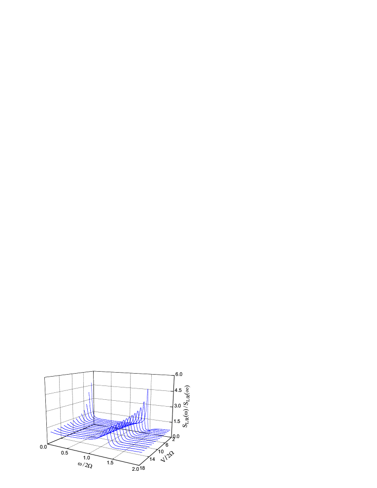
Figure 2: Noise spectral of junction currents scaled by its own pedestal at different measurement voltages for an asymmetrical SET detector with $\Gamma_{\rm R}/\Gamma_{\rm L}=10$ and $\tilde{E}/2\Omega=10$.

III.3 Current noise spectrum

In continuous weak measurement of qubit oscillations, the most important output is the spectral density of the current. The circuit current of the SET detector, according to the Ramo-Shockley theorem,Blanter and Büttiker (2000) is $I(t)=\eta_{\rm L}I_{\rm L}+\eta_{\rm R}I_{\rm R}$, where the coefficients $\eta_{\rm L}$ and $\eta_{\rm R}$ depend on junction capacitances and satisfy $\eta_{\rm L}+\eta_{\rm R}=1$. Together with the charge conservation law $I_{\rm L}=I_{\rm R}+\dot{Q}$, where $Q$ represents the electron charge in the SET dot, one readily obtains $I(t)I(0)=\eta_{\rm L}I_{\rm L}(t)I_{\rm L}(0)+\eta_{\rm R}I_{\rm R}(t)I_{\rm R}(0)-\eta_{\rm L}\eta_{\rm R}\dot{Q}(t)\dot{Q}(0)$. Accordingly, the circuit noise spectral is a sum of three partsJiao et al. (2009); Luo et al. (2007); Gurvitz et al. (2005); Aguado and Brandes (2004)

$$S(\omega)=\eta_{\rm L}S_{\rm L}(\omega)+\eta_{\rm R}S_{\rm R}(\omega)-\eta_{\rm L}\eta_{\rm R}S_{\rm ch}(\omega),$$ (6)

with $S_{\rm L(R)}(\omega)$ the noise spectral of the left (right) junction current, and $S_{\rm ch}(\omega)$ the charge fluctuations in the SET dot. The noise spectral of tunneling current $S_{\rm L/R}$ can be evaluated via the MacDonald’s formulaMacDonald (1962); Flindt et al. (2005); Elattari and Gurvitz (2002)

$$S_{\ell}(\omega)=2\omega\int_{0}^{\infty}\!\!dt\sin(\omega t)\frac{d}{dt}[\langle n_{\ell}^{2}(t)\rangle-(\bar{I}t)^{2}],$$ (7)

where $\bar{I}\equiv I(t\rightarrow\infty)$ is the stationary current, and $\langle n_{\ell}^{2}(t)\rangle\equiv\sum_{{n_{\rm L}},{n_{\rm R}}}n_{\ell}^{2}P({n_{\rm L}},{n_{\rm R}})$. With the help of the conditional master equation (2), it can be shown that

$$\frac{d}{dt}\langle n_{\ell}^{2}(t)\rangle={\rm Tr}[2{\cal T}^{(-)}_{\ell}N_{\ell}(t)+{\cal T}_{\ell}^{(+)}\rho_{\rm st}].$$ (8)

Here $N_{\ell}(t)$ can be found from Eq. (4a), and $\rho_{\rm st}$ is the stationary solution of the unconditional master equation (5).

The symmetrized spectrum for the charge fluctuation in the SET dot readsLuo et al. (2007)

$$S_{\rm ch}(\omega)=\omega^{2}\int_{-\infty}^{\infty}\!d\tau\langle N(\tau)N+NN(\tau)\rangle e^{{\rm i}\omega\tau},$$ (9)

where $\langle N(\tau)N\rangle\equiv{\rm Tr}{\rm Tr}_{\rm B}[U^{\dagger}(\tau)NU(\tau)N\rho_{\rm st}\rho_{\rm B}]$ with $U(\tau)$ the evolution operator of the entire system and $N$ the electron–number operator of the SET dot. It can be reexpressed as $\langle N(\tau)N\rangle={\rm Tr}[N\varrho(\tau)]$, where the alternative reduced density matrix $\varrho(\tau)\equiv{\rm Tr}_{\rm B}[U(\tau)N\rho_{\rm st}\rho_{\rm B}U^{\dagger}(\tau)]$, under the standard Born approximation, satisfies the same equation as $\rho(t)$, but with initial condition $\varrho(0)=N\rho_{\rm st}$. Finally, the spectral of charge fluctuations is obtained asLuo et al. (2007)

$$S_{\rm ch}(\omega)=2\omega^{2}{\rm Re}\,{\rm Tr}\{N[\tilde{\varrho}(\omega)+\tilde{\varrho}(-\omega)]\},$$ (10)

where $\tilde{\varrho}(\omega)$ is the Fourier transform of $\varrho(t)$, and satisfies

$$-{\rm i}\omega\tilde{\varrho}(\omega)=-{\rm i}{\cal L}\tilde{\varrho}(\omega)-{\cal R}\tilde{\varrho}(\omega)+N\rho_{\rm st}.$$ (11)

IV Results and discussions

In this section, we will focus our analysis on the spectral density of the current. Different from the QPC detectors, the circuit current noise spectral of an SET detector is an appropriate combination of three components, as shown in Eq. (6). Hereafter, we first investigate the spectral of junction current and charge fluctuations, respectively, and then analyze the measurement effectiveness based on the circuit noise spectral.

IV.1 Spectral of junction current

In what follows, we assume a symmetric qubit ($\epsilon=0$), and $E=0$ for simplicity. In continuous weak measurement of qubit oscillation, the signal is manifested in the spectral density of the detector output as a peak at qubit oscillation frequency $2\Omega$. The spectral of junction current at different bias voltages is plotted in Fig. 2 for an asymmetric SET detector with $\Gamma_{\rm R}\gg\Gamma_{\rm L}$. It is of interest to note that the peak reflecting the qubit oscillations shifts with the measurement voltages. In the high voltage regime, the oscillation peak is located approximately at $\omega\approx 2\Omega$. As the measurement voltage decreases, the position of the oscillation peak is strongly deviated. Actually, this unique noise feature originates from the SET detection–induced backaction: renormalization of the qubit parameters. The details are explained below.

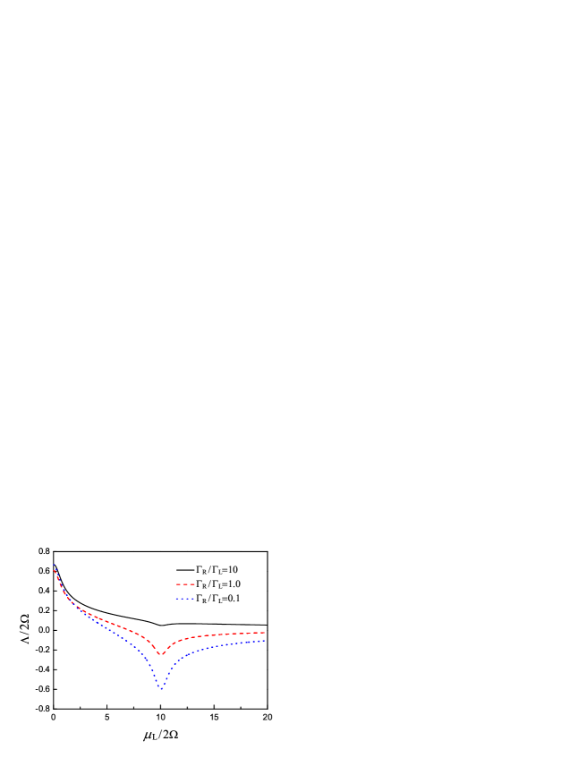
Figure 3: Qubit level renormalization versus measurement voltage at temperature $k_{\rm B}T/2\Omega=0.25$.

The states involved are depicted in Fig. 1. There are totally four eigenstates for the reduced system. The eigen–energies are $\lambda_{+}\pm\Omega$, and $\lambda_{-}\pm\Omega$, respectively, with $\lambda_{\pm}=\frac{1}{2}(\tilde{E}\pm\sqrt{\tilde{E}^{2}+\Omega^{2}})$. Here, we limit our discussions to the strong SET–qubit coupling regime ($\tilde{E}\gg\Omega$). Then the eigen–energies can be markedly reduced, with $\lambda_{+}\pm\Omega\approx\lambda_{+}$ and $\lambda_{-}\pm\Omega\approx\lambda_{-}$. In the bias regime $\lambda_{+}>\mu_{\rm L}>\lambda_{-}>\mu_{\rm R}$, the quantum master equation describing the reduced dynamics can be greatly simplified. Let us denote the density matrix elements by $\rho_{jj^{\prime}}$, with $j,j^{\prime}=${a,b,c,d}. The diagonal terms of the density matrix $\rho_{jj}$ are the probabilities of finding the system in one of the electron configurations (states) as shown in Fig. 1. The off–diagonal matrix elements (“coherencies”), describe the linear superposition of these states. The quantum master equation in this representation simply reads

$$\dot{\rho}_{\rm aa} = \Gamma_{\rm R}\rho_{\rm cc}-\Gamma_{\rm L}\rho_{\rm aa}+{\rm i}\Omega(\rho_{\rm ab}-\rho_{\rm ba}),$$ (12a)

$$\dot{\rho}_{\rm bb} = (\Gamma_{\rm L}+\Gamma_{\rm R})\rho_{\rm dd}-{\rm i}\Omega(\rho_{\rm ab}-\rho_{\rm ba}),$$ (12b)

$$\dot{\rho}_{\rm cc} = \Gamma_{\rm L}\rho_{\rm aa}-\Gamma_{\rm R}\rho_{\rm cc}+{\rm i}\Omega(\rho_{\rm cd}-\rho_{\rm dc}),$$ (12c)

$$\dot{\rho}_{\rm dd} = -(\Gamma_{\rm L}+\Gamma_{\rm R})\rho_{\rm dd}-{\rm i}\Omega(\rho_{\rm cd}-\rho_{\rm dc}),$$ (12d)

$$\dot{\rho}_{\rm ab} = {\rm i}\Omega(\rho_{\rm aa}-\rho_{\rm bb})+{\rm i}\Lambda(\rho_{\rm ab}-\rho_{\rm cd})$$ (12e)

$$+\left(\frac{1}{2}\Gamma_{\rm L}+\Gamma_{\rm R}\right)\rho_{\rm cd}-\frac{1}{2}\Gamma_{\rm L}\rho_{\rm ab},$$

$$\dot{\rho}_{\rm cd} = {\rm i}\Omega(\rho_{\rm cc}-\rho_{\rm dd})+{\rm i}\tilde{E}\rho_{\rm cd}-{\rm i}\Lambda(\rho_{\rm ab}-\rho_{\rm cd})$$ (12f)

$$-\left(\frac{1}{2}\Gamma_{\rm L}+\Gamma_{\rm R}\right)\rho_{\rm cd}+\frac{1}{2}\Gamma_{\rm L}\rho_{\rm ab},$$

where the involving Fermi functions in the tunneling rates are approximated by either one or zero. By observing the equations of motion of the off–diagonal matrix elements [Eqs. (12e) and (12f)], one finds that the qubit level detuning are renormalized, i.e., $\epsilon\rightarrow\epsilon+\Lambda$ with $\Lambda=\sum_{\ell={\rm L,R}}\{\phi_{\ell}(\lambda_{+})-\phi_{\ell}(\lambda_{-})\}$, and

$$\phi_{\ell}(\omega)=\frac{\Gamma_{\ell}}{2\pi}\,{\rm Re}\!\left[\Psi\left(\frac{1}{2}+{\rm i}\frac{\omega-\mu_{\ell}}{2\pi k_{{\rm B}}T}\right)\right].$$ (13)

Here $\Psi$ is the digamma function, $\mu_{\ell}$ is the chemical potential of the SET electrode $\ell\in${L,R}, $k_{\rm B}$ the Boltzmann constant, and $T$ the temperature.

In Fig. 3, the backaction–induced renormalization is plotted against the measurement voltage. The energy shift is closely related to the tunnel–coupling asymmetry and depends on the level positions of the reduced system relative to the Fermi energy. It is found that $\Lambda$ reaches a local extremum, each time when the Fermi energy of the left lead becomes resonant with the eigen–energies, $\mu_{\rm L}=\lambda_{-}$ or $\mu_{\rm L}=\lambda_{+}$. Furthermore, the local minimum at $\lambda_{+}$ is markedly affected by the tunnel–tunneling asymmetry, i.e., the dip is more pronounced as the ratio $\Gamma_{\rm R}/\Gamma_{\rm L}$ decreases.

It is right the shift of qubit level that results in a renormalized Rabi frequency given by $\omega_{\rm R}=\sqrt{\Lambda^{2}+(2\Omega)^{2}}$. It grows with decreasing measurement voltages, as implied in Fig. 3. Eventually, the spectral of junction current $S_{\rm L/R}(\omega)$ exhibits the unique feature that the peak reflecting qubit oscillation shifts with measurement voltages, as shown in Fig. 2.

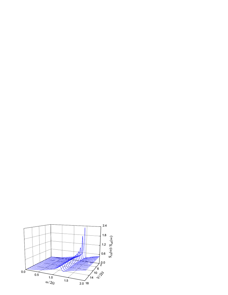
Figure 4: Spectral of charge fluctuations scaled by its own pedestal for different measurement voltages. The plotting parameters are the same as in Fig. 2.

Nevertheless, the bias–dependent peak is not the sole interesting behavior due to the backaction–induced energy shift. Another noticeable feature arising from the level renormalization is the appearance of the noise peak at zero frequency. It is known, that the peak at zero frequency is a signature of the quantum Zeno effect, which indicates the inhibition of transitions between quantum states due to continuous measurement.Korotkov and Averin (2001); Shnirman et al. (2002); Gurvitz et al. (2003) The basic picture is that, due to a strong renormalized level shift, the detector is more readily to localize the electron in one of the levels for a longer time, leading thus to incoherent jumps between the two levels. Yet, the qubit coherence is not strongly destroyed. Eventually, the zero–frequency peak and the coherent peak coexist in the low bias regime, as shown in Fig. 2. This intriguing feature is different from that in the previous work,Gurvitz and Berman (2005); Jiao et al. (2009) where the zero–frequency peak is not observed.

IV.2 Measurement effectiveness

In continuous weak measurement of quantum coherent oscillations of a qubit, an interesting feature of the output noise spectral is that the peak–to–pedestal (“signal–to–noise”) ratio provides the measure of detector “ideality”, i.e., shows how close the detector can be quantum limited. For a perfectly efficient linear detector the maximum peak height can reach 4 times than the noise pedestal, which is universal and known as Korotkov–Averin bound.Jiao et al. (2009); Korotkov and Averin (2001); Korotkov (2001a); Goan and Milburn (2001); Korotkov (2001b) Physically, this limit arises from the tendency of quantum measurement to localize the system in one of the measured eigenstates. So far, many schemes such as quantum nondemolition measurement,Averin (2002); Jordan and Büttiker (2005a) quantum feedback control,Wang et al. (2007) and measurement by using two detectorsJordan and Büttiker (2005b) have been proposed to overcome this bound.

Different from that of a QPC detector, the circuit noise spectral of an SET detector, however, consists of three parts as shown in Eq. (6). It is therefore of vital importance to investigate the charge fluctuations in the SET dot, which uniquely characterizes the current fluctuations in SET dot, and is intimately associated with the qubit dynamics. The numerical result of the charge fluctuations at different measurement voltages is displayed in Fig. 4. At low frequencies the charge fluctuations are strongly suppressed. The most prominent signal is the qubit oscillation peak which is located at the renormalized Rabi frequency $\omega_{\rm R}$, and varies with measurement voltages. It is important to note that the charge fluctuations has an essential role to play in the signal–to–noise ratio, which will be revealed later.

With the knowledge of the junction current noise and the spectral of charge fluctuations, the circuit noise can be readily obtained. It allows us to evaluate the signal–to–noise ratio

$${\rm SNR}=\frac{S(\omega_{\rm R})-S_{0}}{S_{0}},$$ (14)

where $S_{0}\equiv S(\omega\rightarrow\infty)$ is the pedestal of circuit noise. The numerical result of SNR versus tunnel–coupling asymmetry $\Gamma_{\rm R}/\Gamma_{\rm L}$ is plotted in Fig. 5, where we have assumed symmetric capacitive–coupling ($\eta_{\rm L}=\eta_{\rm R}=\frac{1}{2}$). In this case, the influence of charge fluctuations on the circuit noise is maximized.

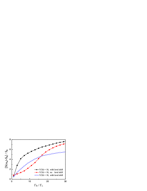
Figure 5: ”Signal–to–noise” ratio versus the degree of tunnel–coupling asymmetry $\Gamma_{\rm R}/\Gamma_{\rm L}$ for different measurement voltages. Other plotting parameters are the same as in Fig. 2.

A remarkable feature observed is that the SNR can exceed “4”, i.e., the upper bound for any linear–response detectors.Korotkov and Averin (2001) This seems to be at variance with Ref. Gurvitz and Berman, 2005, which predict that the effectiveness of an asymmetric SET detector can not reach that of an ideal detector. Here the large spectral of charge fluctuations is responsible for the violation of the Korotkov-Averin bound, as its pedestal can markedly reduces that of the circuit noise [cf. Eq. (6)]. The SNR is thereby enhanced, and finally exceeds the upper bound “4”. Recently, a measurement scheme of a charge qubit with two quantum point contacts was proposed by Jordan and Büttiker.Jordan and Büttiker (2005b) They also observed the violation of the Korotkov–Averin bound, which is ascribed to the negligible small spectral of junction cross–correlations.Jiao et al. (2009); Jordan and Büttiker (2005b) By heuristically viewing the left and right SET electrodes as separate detectors, their analysis qualitatively support our results.

To clearly demonstrate the effect of level renormalization, in Fig. 5 we have also displayed the result in the absence of energy shift. It is found that the renormalization can strongly enhance the SNR. Particularly, in the regime of low $\Gamma_{\rm R}/\Gamma_{\rm L}$ ratio, the effectiveness exceeds the Korotkov–Averin bound purely due to the energy renormalization. It suggests that an ideal SET detector can be achieved even though the tunnel–coupling is not strongly asymmetric. This finding is different from that in Ref. Jiao et al., 2009, where a very large tunnel–coupling asymmetry is required to overcome the Korotkov–Averin bound.

Finally, let us accentuate the influence of the measurement voltage on the signal–to–noise ratio. At a relative large voltage (e.g. $V/2\Omega=18$), the state (d) shown in Fig. 1 becomes partially available at finite temperature. The dynamics of the system is described by the corresponding master equation, which is similar to Eq. (12), but with the crucial difference of an increased decoherence rate. Yet, such an increasing of the decoherence rate is associated with the detector shot noise, rather than the information flow.Clerk et al. (2003); Gurvitz and Berman (2005); Korotkov (2001a, b) Eventually, as shown in Fig. 5, the signal–to–noise ratio is reduced in comparison with that in the lower voltage situation.

V Summary

In summary, the problem of qubit measurements by a single electron transistor detector is investigated, with special attention being paid to the renormalization effect. Our analysis reveals that the dynamical renormalization, which was neglected in previous studies, can strikingly influence the spectral of the detector output. It is therefore of essential importance to take this effect into consideration for correct analyzing and understanding the measurement results. Under proper tunnel–coupling asymmetry, the effectiveness of the single electron transistor detector can be considerably increased. Remarkably, it is observed that the signal–to–noise ratio can exceed the universal Korotkov–Averin bound due purely to the dynamical renormalization.

Acknowledgements

Support from the National Natural Science Foundation of China (Grants Nos. 10904128 and 11004124) is gratefully acknowledged.

References

- Loss and DiVincenzo (1998) D. Loss and D. P. DiVincenzo, Phys. Rev. A 57, 120 (1998).
- Kane (1998) B. E. Kane, Nature 393, 133 (1998).
- Aleiner et al. (1997) I. L. Aleiner, N. S. Wingreen, and Y. Meir, Phys. Rev. Lett. 79, 3740 (1997).
- Gurvitz (1997) S. A. Gurvitz, Phys. Rev. B 56, 15215 (1997).
- Buks et al. (1998) E. Buks, R. Schuster, M. Heiblum, D. Mahalu, and V. Umansky, Nature 391, 871 (1998).
- Goan et al. (2001) H. S. Goan, G. J. Milburn, H. M. Wiseman, and H. B. Sun, Phys. Rev. B 63, 125326 (2001).
- Averin and Sukhorukov (2005) D. V. Averin and E. V. Sukhorukov, Phys. Rev. Lett. 95, 126803 (2005).
- Pilgram and Büttiker (2002) S. Pilgram and M. Büttiker, Phys. Rev. Lett. 89, 200401 (2002).
- Clerk et al. (2003) A. A. Clerk, S. M. Girvin, and A. D. Stone, Phys. Rev. B 67, 165324 (2003).
- Li et al. (2005a) X.-Q. Li, P. Cui, and Y. J. Yan, Phys. Rev. Lett. 94, 066803 (2005a).
- Luo et al. (2009) J. Y. Luo, H. J. Jiao, F. Li, X.-Q. Li, and Y. J. Yan, J. Phys.: Cond. Matt. 21, 385801 (2009).
- Shnirman and Schön (1998) A. Shnirman and G. Schön, Phys. Rev. B 57, 15400 (1998).
- Makhlin et al. (2001) Y. Makhlin, G. Schön, and A. Shnirman, Rev. Mod. Phys. 73, 357 (2001).
- Clerk et al. (2002) A. A. Clerk, S. M. Girvin, A. K. Nguyen, and A. D. Stone, Phys. Rev. Lett. 89, 176804 (2002).
- Jiao et al. (2007) H. Jiao, X.-Q. Li, and J. Y. Luo, Phys. Rev. B 75, 155333 (2007).
- Gilad and Gurvitz (2006) T. Gilad and S. A. Gurvitz, Phys. Rev. Lett. 97, 116806 (2006).
- Gurvitz and Berman (2005) S. A. Gurvitz and G. P. Berman, Phys. Rev. B 72, 073303 (2005).
- Jiao et al. (2009) H. Jiao, F. Li, S.-K. Wang, and X.-Q. Li, Phys. Rev. B 79, 075320 (2009).
- Oxtoby et al. (2006) N. P. Oxtoby, H. M. Wiseman, and H.-B. Sun, Phys. Rev. B 74, 045328 (2006).
- Ye et al. (2010) Y. Ye, J. Ping, H. Jiao, S.-S. Li, and X.-Q. Li, LANL e-print arXiv:10050726 (2010).
- Devroret and Schoelkopf (2000) M. H. Devroret and R. J. Schoelkopf, Nature 406, 1039 (2000).
- Schoelkopf et al. (1998) R. J. Schoelkopf, P. Wahlgren, A. A. Kozhevnikov, P. Delsing, and D. E. Prober, Science 280, 1238 (1998).
- Korotkov and Averin (2001) A. N. Korotkov and D. V. Averin, Phys. Rev. B 64, 165310 (2001).
- Li et al. (2005b) X.-Q. Li, J. Y. Luo, Y. G. Yang, P. Cui, and Y. J. Yan, Phys. Rev. B 71, 205304 (2005b).
- Luo et al. (2007) J. Y. Luo, X.-Q. Li, and Y. J. Yan, Phys. Rev. B 76, 085325 (2007).
- Luo et al. (2008) J. Y. Luo, X.-Q. Li, and Y. J. Yan, J. Phys.: Cond. Matt. 20, 345215 (2008).
- Li et al. (2009) F. Li, H. J. Jiao, J. Y. Luo, X.-Q. Li, and S. A. Gurvitz, Physica E 41, 1707 (2009).
- Xu and Yan (2002) R. X. Xu and Y. J. Yan, J. Chem. Phys. 116, 9196 (2002).
- Yan and Xu (2005) Y. J. Yan and R. X. Xu, Annu. Rev. Phys. Chem. 56, 187 (2005).
- Caldeira and Leggett (1983) A. O. Caldeira and A. J. Leggett, Physica A 121, 587 (1983).
- Weiss (2008) U. Weiss, Quantum Dissipative Systems (World Scientific, Singapore, 2008), 3rd ed.
- Blanter and Büttiker (2000) Y. M. Blanter and M. Büttiker, Phys. Rep. 336, 1 (2000).
- Gurvitz et al. (2005) S. A. Gurvitz, D. Mozyrsky, and G. P. Berman, Phys. Rev. B 72, 205341 (2005).
- Aguado and Brandes (2004) R. Aguado and T. Brandes, Phys. Rev. Lett. 92, 206601 (2004).
- MacDonald (1962) D. K. C. MacDonald, Noise and Fluctuations: An Introduction (Wiley, New York, 1962), ch. 2.2.1.
- Flindt et al. (2005) C. Flindt, T. Novotný, and A.-P. Jauho, Physica E 29, 411 (2005).
- Elattari and Gurvitz (2002) B. Elattari and S. A. Gurvitz, Phys. Lett. A 292, 289 (2002).
- Shnirman et al. (2002) A. Shnirman, D. Mozyrsky, and I. Martin, LANL e-print cond-mat/0211618 (2002).
- Gurvitz et al. (2003) S. A. Gurvitz, L. Fedichkin, D. Mozyrsky, and G. P. Berman, Phys. Rev. Lett. 91, 066801 (2003).
- Korotkov (2001a) A. N. Korotkov, Phys. Rev. B 63, 085312 (2001a).
- Goan and Milburn (2001) H. S. Goan and G. J. Milburn, Phys. Rev. B 64, 235307 (2001).
- Korotkov (2001b) A. N. Korotkov, Phys. Rev. B 63, 115403 (2001b).
- Averin (2002) D. V. Averin, Phys. Rev. Lett. 88, 207901 (2002).
- Jordan and Büttiker (2005a) A. N. Jordan and M. Büttiker, Phys. Rev. B 71, 125333 (2005a).
- Wang et al. (2007) S.-K. Wang, J. S. Jin, and X.-Q. Li, Phys. Rev. B 75, 155304 (2007).
- Jordan and Büttiker (2005b) A. N. Jordan and M. Büttiker, Phys. Rev. Lett. 95, 220401 (2005b).