Determining pseudoscalar meson photo-production amplitudes from complete experiments
Abstract
A new generation of complete experiments is focused on a high precision extraction of pseudoscalar meson photo-production amplitudes. Here, we review the development of the most general analytic form of the cross section, dependent upon the three polarization vectors of the beam, target and recoil baryon, including all single, double and triple-polarization terms involving 16 spin-dependent observables. We examine the different conventions that have been used by different authors, and we present expressions that allow the direct numerical calculation of any pseudoscalar meson photo-production observables with arbitrary spin projections from the Chew-Goldberger-Low-Nambu (CGLN) amplitudes. We use this numerical tool to clarify apparent sign differences that exist in the literature, in particular with the definitions of six double-polarization observables. We also present analytic expressions that determine the recoil baryon polarization, together with examples of their potential use with quasi- detectors to deduce observables. As an illustration of the use of the consistent machinery presented in this review, we carry out a multipole analysis of the reaction and examine the impact of recently published polarization measurements. When combining data from different experiments, we utilize the Fierz identities to fit a consistent set of scales. In fitting multipoles, we use a combined Monte Carlo sampling of the amplitude space, with gradient minimization, and find a shallow valley pitted with a very large number of local minima. This results in broad bands of multipole solutions that are experimentally indistinguishable. While these bands have been noticeably narrowed by the inclusion of new polarization measurements, many of the multipoles remain very poorly determined, even in sign, despite the inclusion of data on 8 different observables. We have compared multipoles from recent PWA codes with our model-independent solution bands, and found that such comparisons provide useful consistency tests which clarify model interpretations. The potential accuracy of amplitudes that could be extracted from measurements of all 16 polarization observables has been studied with mock data using the statistical variations that are expected from ongoing experiments. We conclude that, while a mathematical solution to the problem of determining an amplitude free of ambiguities may require 8 observables, as has been pointed out in the literature, experiments with realistically achievable uncertainties will require a significantly larger number.
pacs:
13.60.Le, 13.75.Gx, 13.75.Jz1 Introduction
As a consequence of dynamic chiral symmetry breaking, the Goldstone bosons dress the nucleon and alter its spectrum. Not surprisingly, pseudoscalar meson production has been a powerful tool in studying the spectrum of excited nucleon states. However, such states are short lived and broad so that above the energy of the first resonance, the (1232), the excitation spectrum is a complicated overlap of many resonances. Isolating any one and separating it from backgrounds has been a long-standing problem in the literature.
The spin degrees of freedom in meson photoproduction provide signatures of interfering partial wave strength that are often dramatic and have been useful for differentiating between models of meson production amplitudes. Models that must account for interfering resonance amplitudes and non-resonant contributions are often severely challenged by new polarization data. Ideally, one would like to partition the problem by first determining the amplitudes from experiment, at least to within a phase, and then relying upon a model to separate resonances from non-resonant processes. Single-pseudoscalar photoproduction is described by 4 complex amplitudes (two for the spin states of the photon, two for the nucleon target and two for the baryon recoil, which parity considerations reduce to a total of 4). They are most commonly expressed in terms of the Chew-Goldberger-Low-Nambu (CGLN) [1] amplitudes. To avoid ambiguities, it has been shown [2] that angular distribution measurements of at least 8 carefully chosen observables at each energy for both proton and neutron targets must be performed. While such experimental information has not yet been available, even after 50 years of photoproduction experiments, a sequence of complete experiments are now underway at Jefferson Lab [3, 4], as well as complementary experiments from the GRAAL backscattering source in Grenoble [5, 6] and the electron facilities in Bonn and Mainz, with the goal of obtaining a direct determination of the amplitude to within a phase, for at least a few production channels, notably and possibly .
The four CGLN amplitudes can be expressed in Cartesian (), Spherical or Helicity (), or Transversity () representations. While the latter two choices afford some theoretical simplifications when predicting asymmetries from models [7], when working in the reverse direction, fitting asymmetries to extract amplitudes, such simplifications are largely moot. The four amplitudes in each of these representations are angle dependent. Extracting them directly from experiment would require separate fits at each angle, which greatly limits the data that can be used and requires some model-dependent scheme to constrain an arbitrary phase that could be angle-dependent. The solution to this intractable situation is a Wigner-Eckhart style factorization into reduced matrix elements, multipoles, and simple angle-dependent coefficients from angular momentum algebra. One can then fit the multipoles directly, which both facilitates the search for resonance behavior and allows the use of full angular distribution data at a fixed energy to constrain angle-independent quantities. The price is a significant increase in the number of fitting parameters, but since the excited states of the nucleon are associated with discrete values for their angular momentum, this expansion of variables is inevitable. Here we restrict our considerations to the CGLN representation, which has the simplest decomposition into multipoles [1], equations (15)-(18) below.
In single-pseudoscalar meson photoproduction there are 16 possible observables, the unpolarized differential cross section (), three asymmetries which to leading order enter the general cross section scaled by a single polarization of either beam, target or recoil (, , ), and three sets of four asymmetries whose leading polarization dependence in the general cross section involves two polarizations of either beam-target (BT), beam-recoil (BR), or target-recoil (TR), as in [7]. Expressions for at least some of these observables in terms of the CGLN appear already in earlier papers [8, 9, 11, 12, 13]. In all cases we have found in the literature, the magnitudes of the expressions relating the CGLN to experimental observables are identical, but the signs of some appear to differ. This is only now becoming a significant issue since the sign differences occur in double-polarization observables for which little data have been available until very recently. There is also a set of Fierz identities interrelating the 16 polarization observables, the most complete list being given in [2]. We have found many of the signs in the expressions of this list appear to be incompatible with several of these papers. As we will see below, much of this confusion has its origin in the same symbol, or observable name, being used by different authors to represent different experimental quantities.
Our purpose here is two fold. First we assemble a complete set of relations, defining observables in terms of specific pairs of measurable quantities and providing the most general form of the cross sections in terms of all observables. We then give a consistent set of relations between these experimental observables and the CGLN amplitudes and electromagnetic multipoles [1]. Next, as an illustration of the use of these relations along the path to determining an amplitude, we use recently published results on 8 different observables to carry out a multipole analysis of the reaction, free of model assumptions, and examine the uniqueness of the resulting solutions. Finally, we use mock data to study the potential uniqueness of amplitudes that could be extracted from complete sets of all 16 observables.
There are several coordinate systems in use in the literature and in section 2 we define ours, which is the same as used in the seminal paper by Barker, Donnachie and Storrow (BDS) [7]. In section 3 we present explicit and complete formulae that allow the direct calculation of matrix elements with arbitrary spin projections from CGLN amplitudes or multipoles. In section 4 we present the most general analytic form of the cross section, dependent on the three polarization vectors of the beam, the target and the recoil baryon. The derivation of this cross section expression is summarized in A, and the experimental definitions of the observables in terms of cross sections with explicit polarization orientations is tabulated in B. Using these definitions, we give in section 5 a summary of the variations in similar formulae that appear in literature. While the beam and target polarizations can be controlled in an experiment, the recoil polarization is on a very different footing, in that it arises as a consequence of the angular momentum of the entrance channel and the reaction physics, neither of which is under experimental control. Expressions that determine the recoil baryon polarization are developed in section 6. To evaluate the analytic relations between observables and amplitudes we next use numerical calculations of the expressions in section 3 to fix signs and present the complete set of equations in section 7 that determine the 16 observables from the CGLN amplitudes. The 37 Fierz identities that interrelate the observables are discussed in section 8 and presented with consistent signs in C. In section 9 we utilize the machinery we have assembled to carry out a multipole analysis of the reaction. (Born terms for this process are summarized in D.) In so doing we test the nature of the valley, discuss the role of the arbitrary phase and examine the impact of recently published polarization data and the uniqueness of the multipole solutions from resent data. The accuracy of the data needed for a precise model independent extraction of amplitudes is then investigated in section 10 from a study with mock data on all possible 16 observables with varying levels of statistical precision. Section 11 concludes with a brief summary.
2 Kinematics and coordinate definitions

The kinematic variables of meson photoproduction used in our derivations are specified in figure 1. Some useful relations are :
-
•
The total center of mass (c.m.) energy:
(1) -
•
The laboratory (Lab) energy needed to excite the hadronic system with total c.m. energy :
(2) -
•
The energy of the photon in the c.m. frame:
(3) -
•
The magnitude of the 3-momentum of the meson in the c.m. frame:
(4) -
•
The density of state factor:
(5)
The definitions of polarization angles used in our derivation are shown in figure 2, using the case of K production as an example. The plane is the reaction plane in the center of mass. The figure illustrates the case of linear polarization, with the alignment direction (parallel to the oscillating electric field of the photon) in the plane at an angle , rotating from towards . The target nucleon polarization is specified by polar angle measured from , and azimuthal angle in the plane, rotating from towards . The recoil baryon is in the plane; its polarization is at polar , measured from , and azimuthal in the plane, rotating from to . Following BDS [7], observables involving recoil polarization are specified in the rotated coordinate system with , along the meson c.m. momentum and opposite to the recoil momentum, , and in the scattering plane at a polar angle of relative to .
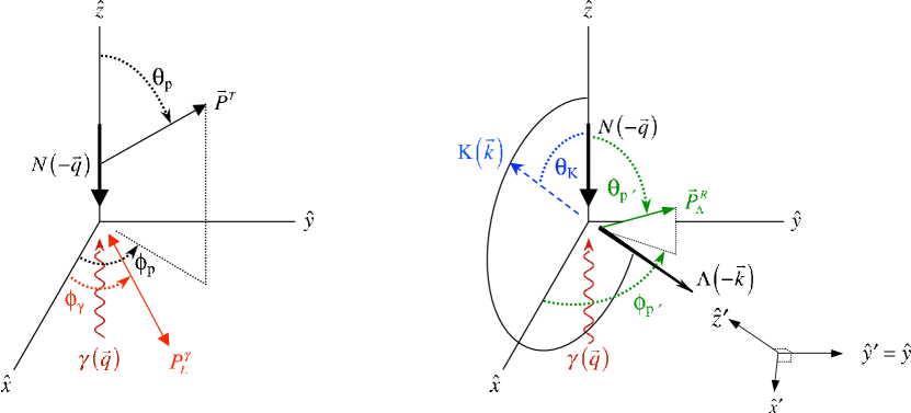
The case of circular photon polarization can potentially lead to some confusion. Most particle physics literature designates circular states as , for right circular (or , for left circular), referring to the fact that with polarization the electric vector of the photon appears to rotate clockwise when the photon is traveling away from the observer. However, when the same photon is viewed by an observer facing the incoming photon the electric vector appears to rotate counter-clockwise. For this reason optics literature traditionally designates this same state as circularly polarized. Nonetheless, both conventions agree on the value of the photon helicity [14] and so we use only the helicity designations here, when 100% of the photon spins are parallel (anti-parallel) to the photon momentum vector.
3 Calculation of polarization observables
As discussed in section 1, all publications give similar formulae for polarization observables, but conflicting signs occur in some terms with very lengthy expressions. It is very difficult, if not impossible, to resolve this problem by repeating the same algebraic procedures used in previous works. To resolve these sign problems, it is necessary to develop completely different and yet simple formulae which can be used to calculate numerically all spin observables of pseudoscalar meson photoproduction. This numerical tool will then allow us to check unambiguously the analytic expressions for spin observables in all previous publications. In this section, we present the derivation of such formulae using the case of photoproduction as an example.
Let us first consider the case when all beam, target, and recoil polarizations are 100% polarized in certain directions. With variables specified as in figure 2, the differential cross section for in the center of mass frame can be written as
| (6) |
where ; with is the photon polarization vector; and are the spin substate quantum numbers of the and the nucleon along the -direction, respectively; is normalized to the usual invariant amplitude calculated from a Lagrangian in the convention of Bjorken and Drell [15]. For example, for a simplified Lagrangian density , the -channel contribution to is . By averaging over all initial state polarizations and summing over final state polarizations in (6), we can obtain the unpolarized cross section:
| (7) |
where the symbol implies taking summation over two photon polarization states, with polarization vectors perpendicular to each other for linearly polarized photons and with helicity states for circularly polarized photons.
The CGLN amplitude [1] is defined by
| (8) |
where is the usual eigenstate of the Pauli operator , and
| (9) |
with
| (10) | |||||
| (11) | |||||
| (12) | |||||
| (13) |
Here we have defined and . We then obtain
| (14) |
The formulae for calculating CGLN amplitudes from multipoles are well known [1] and are given below:
| (15) | |||
| (16) | |||
| (17) | |||
| (18) |
where , is the orbital angular momentum of the system, and and are the derivatives of the Legendre function , with the understanding that . In practice, the sum runs to a limiting value of which depends on the energy.
In order to calculate the 16 polarization observables in an arbitrary experimental geometry, we develop a form for the cross section with arbitrary spin projections for initial and final baryon states, , as specified in figure 2, where () is the unit vector specifying the direction of the target (recoil) spin polarization. Here linear photon polarization must be in the plane and circular photon polarization must be aligned with , while and can be in any directions. The corresponding cross section is obtained by simply replacing in (14) with :
| (19) |
where () is a state of the initial (final) spin- baryon with the spin pointing in the () direction. We note that if () is in the direction of the momentum of the initial (final) baryon, then () is the usual helicity state as defined, for example, by Jacob and Wick [16]. We need to consider more general spin orientations for all possible experimental geometries. The spin state quantized in the direction of an arbitrary vector is defined by
| (20) |
where is the spin operator. For the considered spin-1/2 baryons, is expressed with the Pauli matrix: .
We next derive explicit formulae for calculating the matrix element in terms of the CGLN amplitudes in (15)-(18). We note that the spin state is related to the usual eigenstate of -axis quantization by rotations:
| (21) |
where is defined as , and
| (22) |
We use the phase convention of Brink and Satchler [17] where,
| (23) |
Equation (21) can be easily verified by explicit calculations using the definition (20) and the properties (22) and (23) for the special cases where , , , together with the usual definition of the Pauli matrices, [ and (row), (column) ],
| (24) |
From figure 2, the momenta and linear photon polarization are expressed as
| (25) | |||||
| (26) | |||||
| (27) |
Circular photon polarizations of helicity are expressed as
| (28) |
For the initial and final baryon polarizations, we use the spherical variables, as in figure 2:
| (29) | |||||
| (30) |
By using (25)-(27), we can rewrite in (10)-(13) as
| (31) |
where , , , . The explicit form of is given in table 1.
By using (21) and (9) and (31), the photoproduction matrix element can then be calculated as
| (32) |
with
| (33) |
and
| (34) |
where are the elements of the Pauli matrices of (24).
We may now start with any set of multipoles and use (15)-(18) to calculate the CGLN amplitudes, which are then used to calculate the matrix element with the help of (32)-(34). Equation (19) then allows us to calculate all possible polarization observables, for the case of unit polarization vectors with arbitrary orientation.
With non-unit polarization vectors, the general cross section can be expressed in terms of (19) as, (see also A),
| (35) |
Here the vector specifies the degree and direction of the polarization of particle . For the target (T) and recoil (R) baryons, this is just , where () is the probability of observing with its polarization vector pointing in the direction. For the photons (), however, the non-unit polarization vector can be expressed as . Here, () and are orthogonal polarization directions, apart for linear polarization, and opposite helicity states for circular polarization. Then () is a probability observing photons with its polarization vector pointing in the () direction. To clarify (35), consider the case that all beam, target, and recoil particles are unpolarized as an example. In this case the probabilities of finding spin projection in each of two possible directions are equal and hence , which leads to . Then we have
| (36) | |||||
where is the unpolarized cross section defined in (7). The factor in the last equation appears because the polarization of the final recoil particles is also averaged in (36).
4 General cross section
While the formulae presented in the previous section can be used numerically to calculate any observable of pseudoscalar meson photoproduction, it is more convenient to analyze the data using an analytic expression for the general cross section of equation (35). In terms of the polarization vectors of figure 2, and with signs verified numerically using (35) of section 3, the most general form of the cross section can be written as,
| (37) | |||||
The derivation of this analytic expression is summarized in A, where we follow the formalism of Fasano, Tabakin and Saghai (FTS) [11], expanding their treatment to include the complete set of triple polarization cases. In this expression we have designated the product of an asymmetry and with a caret, so that . These products are referred to as profile functions in [2, 11]. One can of course pull a common factor of out in front of the above expression, in which case all the profile functions are replaced by their corresponding asymmetries. However, we keep the above form since it is the profile functions that are most simply determined by the CGLN amplitudes. (The definition of each of these profile functions in terms of measurable quantities is given by B.) The second, third and fourth terms (, , ) are commonly referred to as single-polarization observables, since their leading coefficients contain only a single polarization vector. The subsequent 12 terms are grouped into 3 sets, each containing four terms, referred to as {BT, BR, TR} according to the combination of polarization vectors appearing in their leading coefficients. Two of the leading terms have negative coefficients. The first arises because we have taken for the numerator of the beam asymmetry () the somewhat more common definition of (), rather than its negative. [Here corresponds to () in the left panel of figure 2.] In the second leading term with a negative coefficient, we have taken the numerator of the asymmetry as the difference of cross sections with anti-parallel and parallel photon and target spin alignments (). This follows a convention first introduced by Worden [18] and propagated through many (though not all) subsequent papers, and has been used in recent experimental evaluations of the GDH sum rules [19]. The specific measurements needed to construct each of these observables are tabulated in B.
Recoil observables are generally specified in the rotated coordinate system with . Occasionally, a particular recoil observable will have a more transparent interpretation in the unprimed coordinate system of figure 2 [20]. Since a baryon polarization transforms as a standard three vector, the unprimed and primed observables are simply related:
| (38) |
and
| (39) |
where represents any one of the BR or TR observables.
It is convenient to arrange the observables entering the general cross section in tabular form, as in table 2. The four rows correspond to different states of beam polarization, either ignoring the incident polarization entirely (labeled unpolarized in table 2), or in one of three standard Stokes vector components that characterize an ensemble of photons with polarization , linear at to the reaction plane (which enters the cross section with a dependence), linear either in or perpendicular to the reaction plane (which enters the cross section with a dependence), or circular. The columns of the table give the polarization of the target, recoil, or target + recoil combination. One can readily construct from this table the terms that enter the general cross section for any given combination of polarization conditions. These consist of the terms involving all applicable polarization vectors, as well as those that survive when initial states are averaged and/or final states are summed. We consider two examples as an illustration. First, for a circularly polarized beam on an unpolarized target with an analysis of the three components of recoil polarization, the general cross section contains terms from the average of initial states (first row of table 2) and from the polarized initial state (forth row). Contributing terms come from only those columns that do not require knowing the target polarization state. Thus the cross section for this condition becomes . Alternatively, with linear beam polarization in or perpendicular to the reaction plane, a longitudinally polarized target (along ) and an analysis of recoil polarization along the meson (kaon) momentum (), the general cross section is given by the terms in the first (unpolarized) and third rows that are either independent of target and recoil polarization (,) or in columns associated with polarization along and/or , namely .
-
Beam () Target () Recoil () Target () + Recoil () unpolarized circular
5 Variations within the existing literature
The form of the general cross section expression in equation (37) has been derived analytically in A and checked numerically with the tools of section 3. At this point, it is instructive to summarize the variations in similar formulae in the literature which have already caused some confusions in analyzing recent data and must be resolved for future development. The most frequently quoted works that discuss the relation between observables and CGLN amplitudes are the following four: Barker-Donnachie-Storrow (BDS) [7], Adelseck-Saghai (AS) [10], Fasano-Tabakin-Saghai (FTS) [11], and Knöchlein-Drechsel-Tiator (KDT) [13]. A few of the differences between them are summarized in the following subsections.
5.1 BDS
The coordinate system of the BDS paper is the same as ours in figure 2 above. The photon beam momentum is along ; is the reaction plane containing the meson momentum emerging at a center of mass angle measured from rotating towards ; and . The recoil baryon polarization is specified in a rotated primed-coordinate system, with along the meson momentum, ; and lies in the plane, rotated down from by . It has since become common to indicate the use of this rotated system by including a prime in the symbol of observables that involve recoil, e.g., , , etc., although the prime is not used in the BDS paper. The BDS paper is certainly a seminal work on this subject but, in its published form, it contains an unfortunate piece of typesetting that has lead to some confusion. Page 348 of that journal article ends with the sentence, “The precise relation between observables and the experiments we consider is as follows.” The next page 349 contains table I with several columns, the “Usual symbol” for the observables, their decomposition into “Helicity” and “Transversity” amplitudes, and in the fourth column the “Experiment required” to measure each observable. This forth column utilizes a notation that is somewhat condensed, but at least appears clear for linear polarization at to the reaction plane. For example the experiment required to determine the asymmetry is listed as , which would imply the following ratio of cross sections with polarized beam, target and recoil,
where unobserved final recoil polarization states are summed. However, equation (2) in BDS [7] at the top of the following page 350 gives the -dependence of the cross section as,
| (40) |
and using this to evaluate the above ratio results in . The sense of rotation for the angle is not defined, but we assume it is measured from the axis rotating toward the axis. [The opposite sense would introduce another negative sign in terms proportional to .] We regard the equation for the cross section as the most definitive. Thus, one should take the “Helicity” and “Transversity” expansions of the observables in the second and third columns of table I in BDS [7] literally, but the required experiment in column four as schematic only, leaving the sign of the specific combination of measurements to be determined from their equations (2)-(4). While rather convoluted, we believe this represents the correct reading of the BDS paper. Finally, we note that equations (3) and (4) in BDS [7], which give their cross sections for polarized beam and recoil, and for polarized target and recoil, respectively, are both missing a factor of . This is easily seen by averaging over initial states and summing over final states, which for the equations as written results in twice the unpolarized cross section, .
5.2 AS
While the BDS coordinates were focused on the meson, the coordinate system of the AS paper is focused on the final state baryon. The photon beam momentum is along . In the reaction plane the recoil baryon emerges at a center of mass angle measured from rotating towards ; is still defined with the meson momentum as , but now . The sense of rotation for the linear photon polarization angle is defined from the axis rotating toward . Relative to , a linear polarization orientation of in AS coordinates corresponds to in BDS and the present work. The primed-coordinate system is taken with along the baryon momentum; and lies in the plane, rotated up from by . The observables involving components of the recoil polarization refer to the primed coordinates, although primes are not included in their notation. The AS paper includes a general expression for the cross section in terms of beam, target and recoil polarizations. However, as discussed in section 6 below, their expression has at least one misprint in its last line, with two terms involving and but none with and . As evident in our equation (37), each of these observables appears in the general cross section with two coefficients, one dependent upon and the other upon .
5.3 FTS
The coordinate system of FTS is the same as that of BDS and of the present work. Circular polarization states are designated as and . Although the Stokes vector for the photon beam is taken from optics (which associates circular polarization with helicity ), their table I associates beam polarization with helicity . The sense of rotation for the linear photon polarization angle is defined from the axis rotating toward . The observables involving components of the recoil polarization are designated with primed symbols. FTS does not give an explicit expression for the cross section in terms of observables and polarizations, but the paper does list explicit definitions of observables in terms of measurable quantities. The FTS paper also gives explicit equations relating the observables to the CGLN amplitudes.
5.4 KDT
The coordinate system of KDT is the same as that of BDS and of the present work.
Circular photon polarization () is referred to as right handed;
although helicity is not discussed, we have assumed (in Table 3 below)
that their right-handed state corresponds to .
The direction of rotation for the angle is not defined;
in the evaluation below we have assumed their azimuthal polarization angle rotates
from toward .
Cross section equations are given for the cases of beam+target polarization,
beam+recoil polarization and target+recoil polarization.
As in BDS, the latter two are missing a factor of , as is easily verified
by averaging over initial states and summing over final states.
KDT provides explicit equations to relate each observable to the CGLN amplitudes.
To completely define an observable in terms of measurable quantities one needs a specification of the coordinate system and either the equation for the cross section in terms of polarizations and observables, or an explicit definition of the observables in terms of measurable cross sections. As an example of some of the variations that have resulted from different conventions, consider the beam+target asymmetries. We can define these as coordinate-independent ratios with directions specified by only photon () and meson () momenta.
| (41) | |||||
| (42) | |||||
| (43) | |||||
| (44) | |||||
with
The variable names of these ratios as used by different authors are listed in table I. As evident there, the same symbol has been used in different papers to refer to different quantities, with common magnitudes but varying signs. This creates the potential for spiraling confusion when a third party combines equations from different papers.
The present work has avoided the confusions associated with variations in formulae from different papers by developing a consistent and self-contained set of expressions that (a) define each observable in terms of measurable cross sections (B), (b) provide the most general expression for the cross section in terms of the 16 observables and the beam, target and recoil polarization states, both derived analytically (A) and checked numerically (sections 3 and 4), and (c) provide the defining relations between the 16 spin observables and the CGLN amplitudes (section 7 below).
6 Recoil polarization
As a first application of the consistent expression of the general cross section presented in section 4, we analyze the potential of experiments measuring recoil polarization. The general expression in (37) displays a level of symmetry in the three polarization vectors, , and . However, while the first two are parameters that are under experimental control, the recoil polarization is not. Rather, is a consequence of the angular momentum brought into the entrance channel through and , and the reaction physics. The relations determining are readily derived. We start by regrouping terms in the general cross section expression to display the explicit dependence on and recast (37) as,
| (45) |
where
The recoil polarization can be resolved as the vector sum of three component vectors, , , . Considering first , this is the degree of polarization along and is given by
| (46) |
where is the probability for observing the recoil with spin along . Using (45), we evaluate this as the ratio of cross sections,
| (47) |
The and recoil components are evaluated in a similar manner. Thus, the components of the recoil polarization are determined from (45), in terms of combinations of the profile functions and initial polarizations, as
| (48) |
These recoil components determine the orientation of the recoil vector, , and its magnitude,
| (49) |
It is worth clarifying the relationship between (37) or (45) and (48). Equations (37) and (45) display the general dependence of the cross section upon the three polarization vectors, each of which is in a superposition of two spin states. If any one polarization is not observed, either by not experimentally preparing it ( or ) or by not detecting it (), then the terms proportional to that polarization average or sum to zero and drop out of the cross section. The action of preparing or detecting a polarization forces the corresponding magnetic substate population into a particular distribution, which in the case of the recoil polarization is given by (48). A particular consequence of this is that one may not substitute (48) back into (45) to obtain a cross section that appears to be independent of recoil polarization.
An expression similar in spirit to (45) but different in form is given by Adelseck and Saghai in [10]. However, the coordinate system is very different and there is at least one obvious misprint, with two terms involving and but none with and , as discussed in section 5.2.
In practice, the recoil polarization is measured either following a secondary scattering or, in the case of hyperon channels, through the angular distribution of their weak decays. production provides a particularly efficient channel for recoil measurements. In the rest frame of the decaying , the angular distribution of the decay proton follows , where is the angle between the proton momentum and the lambda polarization direction [21]. Since the analyzing power in this decay is quite high, [22], recoil measurements in modern quasi- detectors can be carried out without significant penalty in statistics. As a result, such measurements provide information on combinations of observables through (48). It is instructive to consider a few examples.
-
1.
Unpolarized beam and target, : In this case, , , and , so that
(50) Thus, even when the initial state is completely unpolarized, a measured recoil polarization will be perpendicular to the reaction plane.
-
2.
Unpolarized beam and longitudinally polarized target, and : In this case, , , , and , so that
(51) Thus a measurement of the components of the recoil polarization determine the , and asymmetries.
-
3.
Circularly polarized beam () and unpolarized target (): In this case, , , , and , so that
(52) This is the form assumed in the analysis of the CLAS-g1c data in [20].
-
4.
Linearly polarized beam () and unpolarized target (): In this case, , , , and , so that
which is the form assumed in the analysis of the GRAAL data in [6], although the coordinate system is different.
-
5.
Circularly polarized beam () and longitudinally polarized target []: In this case, , , , and , so that
(54) Here, measurements with complete knowledge of all spins involved provide the greatest flexibility. An initial beam-target analysis summing over final states (i.e., ignoring the recoil) results in the cross section , which determines the asymmetry and hence the denominator in (54). In an analysis averaging over initial target polarizations , measurements of the recoil polarization vector then determine the , and asymmetries. Another pass through the data, averaging instead over initial beam polarization states, , and with an analysis of the and recoil components, gives the and asymmetries. Finally, by keeping track of both beam and target polarization states, a measurement of the recoil component gives the asymmetry. Although the uncertainty in this determination of will include the propagation of errors from and , this is expected to be held to a reasonable level in the modern set of experiments that are now under way. The significance of this determination is that it does not require the use of a transversely polarized target, as would otherwise be required by the leading polarization dependence of in (37). In general, the latter would require a completely separate experiment with different systematics.
-
6.
Linearly polarized beam () and longitudinally polarized target []: In this case, , , , and , so that
(55) With such data a beam-target analysis summing over final states (i.e., ignoring the recoil) determines the cross section , and hence the and asymmetries from a Fourier analysis of the dependence. This fixes the denominators in (55). With another analysis pass, averaging over initial target polarizations, measurements of the recoil polarization vector provide a determination of the , and , and asymmetries. Another pass through the same data, integrating over , gives the , and asymmetries from measurements of the recoil polarization vector. Finally, a Fourier analysis of beam polarization states, using the difference between opposing target orientations, , together with a measurement of recoil polarization allows the separation of and , (which would otherwise require a transversely polarized target), and and .
Thus, by judicious use of recoil polarization and a polarized beam, all 16 observables can be determined with a longitudinally polarized target (often in several ways) and in doing so, with largely common systematics.
A corresponding set of expressions can be developed for a transversely polarized target, although they are inherently more complicated since, for fixed target polarization perpendicular to , any reaction plane will generally involve both transverse target components and .
-
7.
Unpolarized beam () with a transversely polarized target and []: In this case, , , , and , so that
(56) Here an analysis summing over final states (i.e., ignoring the recoil) results in the cross section , and a fit varying as the reaction plane tilts relative to the direction of the target polarization determines the asymmetry. A subsequent analysis of the recoil polarization components then determines , , , and .
-
8.
Circularly polarized beam () and transverse target polarization []: In this case, , , , and , so that
(57) In this case, a beam-target analysis summing over final states (i.e., ignoring the recoil) results in the cross section containing the terms in the and asymmetries, and these can be separated by first averaging over initial photon states, which removes . A subsequent analysis, reconstructing the recoil polarization while averaging over initial circular photon states allows one to deduce and from and . Alternatively, with fixed beam polarization and recoil analysis, a fit varying and as the reaction plane tilts in azimuth relative to the direction of the transversely polarized target determines all of the asymmetries in the numerators of (57).
We leave it to the reader to write out the final combination of linearly polarized beam and transverse target polarization. There the recoil polarization components involve ratios of 4 to 5 terms each. It remains to be seen if sequential analyses of such data are of practical use, given limitations on statistics.
7 Relating observables to CGLN amplitudes
To extract nucleon resonances, one needs to extract amplitudes from observables. Because of the apparent variations in the available literature, as summarized in section 5, there exists sign differences in formula relating observables to CGLN amplitudes. With the formula presented in sections 3 and 4, we are now in a position to clarify this issue. This is done by using any set of multipole amplitudes to calculate the four CGLN amplitudes from (15)-(18) and then with these, evaluate (a) the polarization observables by using the formulae described in section 3 and the spin orientations specified in the tables of B, and (b) the same observables calculated from the analytic expressions, as found in [8, 9, 11, 12, 13]. As expected, the absolute magnitudes from the two methods are the same, but some of their signs are different. In doing so, we are able to fix the signs of the analytic expressions for the experimental conditions specified in figure 2 and B. Our results are:
| (58a) | |||
| (58b) | |||
| (58c) | |||
| (58d) | |||
| (58e) | |||
| (58f) | |||
| (58g) | |||
| (58h) | |||
| (58i) | |||
| (58j) | |||
| (58k) | |||
| (58l) | |||
| (58m) | |||
| (58n) | |||
| (58o) | |||
| (58p) | |||
A comparable set of expressions are given by Fasano, Tabakin and Saghai (FTS) in [11]. With the conventions discussed in section 5.3, and allowing for their different definition of the beam-target asymmetry (as in table 3), the above expressions are consistent with those of [11].
Comparing the above relations to those given by Knöchlein, Drechsel and Tiator (KDT) (Appendix B and C of [13]), six of these equations have different signs, the BT observable , the TR observable and all four of the BR observables , , and . The KDT paper [13] is listed in the MAID on-line meson production analysis [23, 24, 25] as the defining reference for their connection between CGLN amplitudes and polarization observables. To check if these differences persist in the MAID code we have downloaded MAID multipoles, used the relations in (15)-(18) to construct from these the four CGLN amplitudes, and then used our equations (58a)-(58p) above to construct observables. Comparing the results to direct predictions of observables from the MAID code, we find the same six sign differences. However, KDT give a form of the general cross section with leading polarization terms in [13] and there, the equations for these six observables appear with a negative coefficient, as opposed to our form of the cross section in (37). This is equivalent to interchanging the and measurements of B that are needed to construct these six quantities. (Such differences were already discussed in section 5 above, with the asymmetry as an example.) Thus, KDT use the same six observable names as the present work to refer measurable quantities of the same magnitude but opposite sign.
We have conducted a similar test with the GWU/VPI SAID on-line analysis code [26, 27], downloading SAID multipoles, using the relations in (15)-(18) to construct from these the four CGLN amplitudes, and then using our equations (58a)-(58p) above to construct observables. When the results are compared to direct predictions of observables from the SAID code, again the same 6 observables differ in sign. For the definition of observables, SAID refers to the Barker, Donnachie and Storrow paper [7]. As discussed in section 5, the BDS definitions of asymmetries should be deduced from their equations (2)-(4) and these have signs consistent with KDT. Thus SAID also uses the same six observable names as the present work to refer to quantities of the same magnitude but opposite sign.
We have repeated this same test with the Bonn-Gatchina (BoGa) on-line PWA [28], downloading BoGa multipoles, using the relations of (15)-(18) to construct the four CGLN amplitudes, and then using our (58a)-(58p) to construct observables. Comparing these to direct predictions of observables from the BoGa code, the results are identical, except for the asymmetry which is of opposite sign. However, for the definition of observables the BoGa on-line site refers to FTS of [11], whose definitions are the same as in our B except for a sign change in the asymmetry, as in table 3. Thus, we conclude that the relations between observables and amplitudes used in the BoGa analysis is completely consistent with the present work.
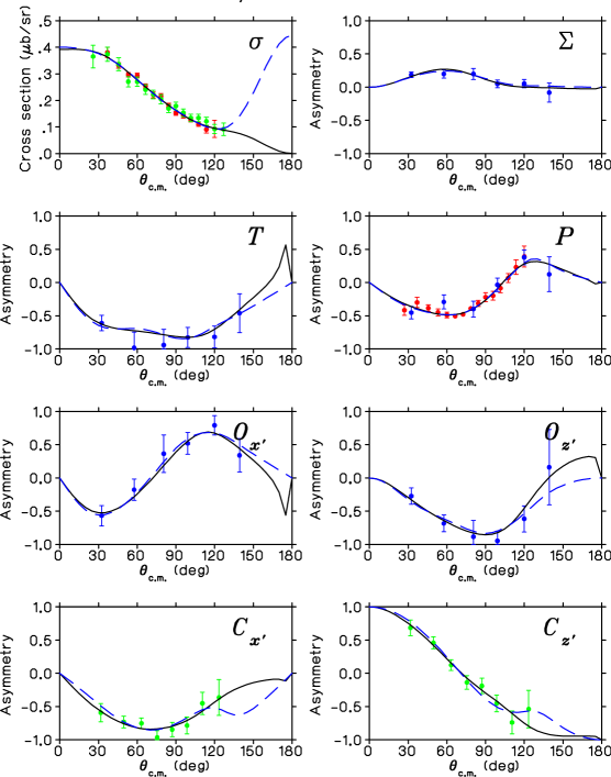
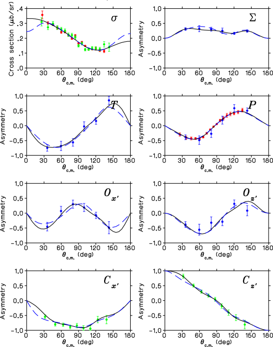
New data are emerging from the current generation of polarization experiments which make these sign differences an important issue. In [20], recent results for the and asymmetries have been compared with the direct predictions of the Kaon-MAID code, with predictions from an earlier version of the BoGa multipoles and with predictions from Juliá-Díaz, Saghai, Lee and Tabakin (JLST) [29]. As an illustration, in figure 3 we have replotted figures 8 and 9 from [20] for two energies, transformed to the primed kaon axes using equation (39), and added the predictions from SAID. The MAID (black dashed) and SAID (black, dotted) curves for approach at , while the BoGa (blue, dot-dashed) and JSLT (blue, solid) curves approach , along with the data (green circles) from [20].
The behavior of at is a simple reflection of angular momentum conservation. Using the definition from B, . When the incident photon spin is oriented along , only those target nucleons with anti-parallel spin can contribute to the production of spin zero mesons at , and the projection of the total angular momentum along is . Thus, the recoil baryon must have its spin oriented along at , so that must vanish. The recent measurements on production [20] clearly show this asymmetry approaching at .
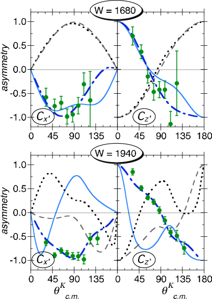
The MAID and SAID predictions appear to have the wrong limits for at 0 and 180 degrees. Also shown are predictions using the multipoles of Juliá-Díaz, Saghai, Lee and Tabakin (JSLT) from [29], used with our expressions to construct observables (solid blue curves). The MAID and SAID sign differences are also evident in , particularly at low energies where only a few partial waves are contributing - top panels of figure 3. There it is clear that the predictions of the different partial wave solutions are essentially very similar, differing only in sign. The comparisons of [20], repeated here in figure 3, illustrate the confusion that arises from the use of the same symbol to mean different experimental quantities by different authors (section 5).
8 Relations between observables
Since photo-production is characterized by 4 complex amplitudes, equation (9), the 16 observables of equations (58a)-(58p) are not independent. There are in fact many relations between them. The profile functions of (58a)-(58p) are bilinear products of the CGLN amplitudes, and one of the more extensive sets of equalities interrelating them has been derived by Chiang and Tabakin from the Fierz identities that relate bilinear products of currents [2]. Such relations are particularly useful, since they allow the comparison of data on one observable with an evaluation in terms of products of other observables. Any determination of the amplitude will invariably require combining data on different polarization observables which in general come from different experiments, each having different systematic scale uncertainties. The Fierz identities provide a means of enforcing consistency provided, of course, that they are consistent with the expressions of general cross sections given in section 4.
The Fierz identities as derived by Chiang and Tabakin (CT) are given in terms of 16 quantities, in [2], and the first column of table I in that paper gives the relation between these quantities and the conventional single, BT, BR and TR observable names. CT quote FTS for the definition of these observables. We have numerically checked the 37 Fierz identities of Appendix D in [2]. Assuming the definitions of observables as given in our B, or in FTS, a large number (more than half of them) require revisions in signs. If the signs of are reversed, as in BDS and KDT, still many of the equations of [2] require revision. A set of identities that are consistent with our definitions of observables in terms of measurable quantities, B, and with the form of our general cross section in equation (37), is given below in the first three sections of C. As a practical example, in the next section we use two of the identities in a multipole analysis to fix the scales of different data sets in a fit weighted by their systematic errors.
Another set of relations has been given by Artru, Richard and Soffer (ARS) [30, 31]. These are different in form but can be derived from our Fierz identities, although with some differences in signs. A consistent set is listed in C.4.
In addition to identities, there are a number of inequalities, such as , which are often referred to as positivity constraints [30]. These involve the sums of the squares of asymmetries, and as such are immune to sign issues. They can be particularly useful when extracting sets of asymmetries from fits to experimental data [32], as in the examples discussed in section 6. But since our focus here is amplitude reduction from cross sections and asymmetries, we refer the reader to a recent review of such inequalities [31].
9 Multipole analyses
The ultimate goal of the new generation of experiments now under way is a complete experimental determination of the multipole decomposition of the full amplitude in pseudoscalar meson production. In this section, we apply the formula presented in previous sections to develop this analysis process as model independently as possible. While the data published to date are still insufficient to satisfy the Chiang and Tabakin requirements for removing discrete ambiguities [2], it is instructive to examine the impact of recently published polarization measurements. We focus here on the channel, which so far has provided the largest number of different observables, as summarized in table 4.
To avoid bias, the first stage in any multipole decomposition is a single-energy analysis, one beam/ energy at a time without any assumptions on energy-dependent behavior. The range of recent published measurements is summarized in table 4. [Cross section data from the SAPHIR detector at Bonn [33] have an appreciable (20%) angle- and energy-dependent difference from the CLAS experiments. This level of incompatibility makes it impossible to include them in the present analyses.] While some of the data sets span the full nucleon resonance region in extremely fine steps, single-energy analyses are limited by the observables with the coarsest granularity, which in this case are the , measurements (data group 3 [20]). The only published , and data are from GRAAL (data groups 5 and 8 [6]). The combination of these data sets allows us to combine groups 1-8 at 5 different beam energies, with roughly 100 MeV steps in beam energy, for which 8 different observables are now available.
| Data | Experiment | Observables | range (MeV) | / | Systematic |
|---|---|---|---|---|---|
| group | range (MeV) | binning | scale error | ||
| 1 | CLAS-g11a [34] | 938-3814 | % | ||
| 1625-2835 | 10 | ( dep.) | |||
| 2 | CLAS-g11a [34] | 938-3814 | |||
| 1625-2835 | 10 | ||||
| 3 | CLAS-g1c [20] | , | 1032-2741 | 101 | |
| 1679-2454 | |||||
| 4 | CLAS-g1c [35] | 944-2950 | 25 | % | |
| 1628-2533 | ( dep.) | ||||
| 5 | GRAAL [6] | , | 980-1466 | 50 | % |
| 1649-1906 | |||||
| 6 | GRAAL [5] | 980-1466 | 50 | % | |
| 1649-1906 | |||||
| 7 | GRAAL [5] | 980-1466 | 50 | % | |
| 1649-1906 | |||||
| 8 | GRAAL [6] | 980-1466 | 50 | % | |
| 1649-1906 | |||||
| 9 | LEPS [36] | 1550-2350 | 100 | % | |
| 1947-2300 |
9.1 Coordinate transformations
There are several different choices for coordinate systems in use and before data from the different experiments can be combined in a common analysis we transformed them to the system defined in figure 2. The beam-recoil data of group 3 [20] were reported in unprimed c.m. coordinates relative to the beam direction. These are related to the primed system of figure 2 by the relations in equation (39). The GRAAL papers use the coordinates of Adelseck and Saghai [10]. Relative to , their and axes are reversed from those of figure 2, so that, although , and are unchanged in transferring to our coordinates, become the negative of what GRAAL refer to as . Thus,
| (58bg) |
9.2 Constraining systematic scale uncertainties
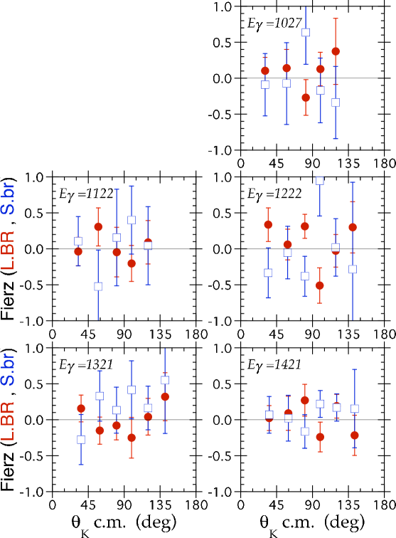
Each experiment has reported systematic errors that reflect an uncertainty in the scale of the entire data set. We use a procedure of imposing self-consistence within a collection of data sets by including their measurement scales as parameters in a fit minimizing [37]. To fix first the scales of the polarization observables, data groups (2,3,5,6,7,8) of table 4, we use the Fierz identities (L.BR) and (S.br) of C to construct the quantities,
| (58bh) |
both of which have the expectation value of 0 at each angle and energy. Our fitting procedure then minimizes the function,
| (58bi) | |||||
where the index runs through each of the data groups of asymmetries () needed to construct the Fierz relations of (58bh). All data from a set having a systematic scale error () are multiplied by a common factor () while adding to the . This last term weights the penalty for choosing a normalization scale different from unity by the reported systematic uncertainty of the experiment.
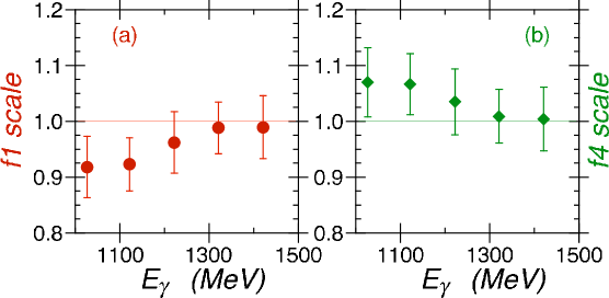
In this procedure polynomial fits are used, where needed, to interpolate the data of table 4 to a common angle and energy. There are two measurements of the recoil polarization asymmetry (), from groups 2 and 6 in table 4, and a weighted mean of these data, including their scale factors, is used in evaluating (58bi). The scale factors resulting from this fit are listed in table 5. All are close to unity. The resulting evaluations of the Fierz relation, using the scaled data, are shown in figure 4.
-
Data group Experiment Observables Fitted scale () Scale error () 2 CLAS-g11a 1.000 0.049 3 CLAS-g1c , 0.984 0.025 5 GRAAL , 0.997 0.035 6 GRAAL 1.001 0.030 7 GRAAL 1.001 0.020 8 GRAAL 0.992 0.040
While the results in figure 4 scatter around zero as expected, the fluctuations are sometimes appreciable. These cannot readily be removed with an energy- and angle-independent scale factor. It is likely this results from combining data from different detectors. While global uncertainties such as flux normalization and target thickness can be readily estimated and easily fitted away in this type of procedure, angle-dependent variations in detector efficiencies tend to be the most problematic to control and quantify.
9.3 Multipole fitting procedure
The observables of table 4 are determined by the CGLN amplitudes through (58a)-(58p), and these are in turn determined by the multipoles through (15)-(18). Since the multipoles are reduced matrix elements and independent of angle, fitting them directly allows the use of complete angular distributions for each observable. We fix the scales () of the polarization observables to their fitted values in table 5, and now vary the multipoles, as well as the scales and for the unpolarized cross section () measurements (groups 1 and 4 in table 4) to minimize the function,
| (58bj) |
where is the number of independent data sets, each having points. and are the -th experimental datum from the -th data set and its associated measurement error, respectively, is the value predicted from the multipole set being fit, and is the global scale parameter associated with the -th data set. As before, the last term weights the penalty for choosing a cross section scale different from unity by the reported systematic uncertainties for data groups 1 and 4 [37].
Thus our fitting procedure is a two-step process, first minimizing (58bi) by varying the scale factors of the polarization data, and then minimizing (58bj) in a second step by varying the multipoles and the cross section scales. These two cannot be combined into a single step in which Fierz relations such as (58bh) are minimized by varying multipoles, since all properly constructed multipoles will automatically satisfy the Fierz identities.
While the cross section experiments report the global systematic uncertainties listed in table 4, comparisons given in [34] show a clear energy dependence to the scale difference between them, which is most pronounced at low energies. Accordingly, we have fitted separate cross section scales at each energy and the results are plotted in figure 5.
Cross sections for any reaction generally fall with increasing angular momentum, which guarantees the ultimate convergence of a multipole expansion. However, in practice such expansions must be truncated to limit the maximum angular momentum to a value that is essentially determined by the statistical precision and breadth of kinematic coverage of the data sets. The ultimate goal of such work will be the identification of the excited states of the nucleon, and this will require, as a minimum, accurate multipole information up to at least to be useful. As has been shown by Bowcock and Burkhardt [38], the highest multipole fitted in any analysis always tends to accumulate the systematic errors stemming from truncation and is essentially guaranteed to be the most uncertain. Thus, when focusing on multipoles up to we must vary up to and fix the multipoles for to their (real) Born values. (Details of the Born amplitudes are given in D.)
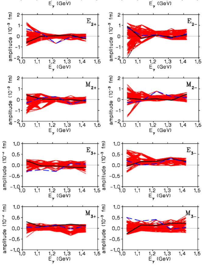
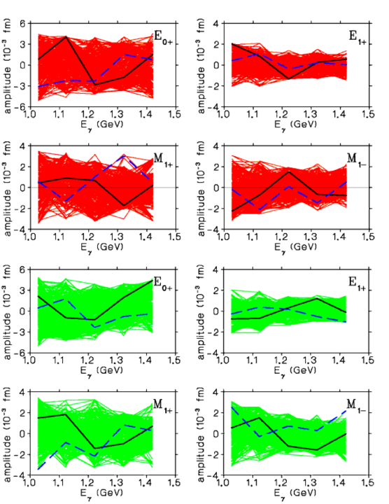
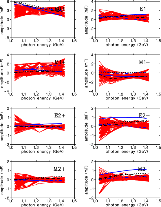
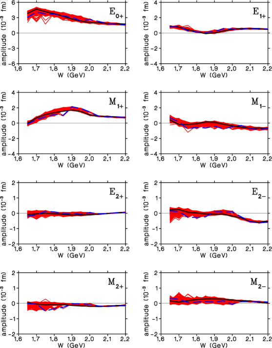
To search for a global minimum while allowing for the presence of local minima, we use a Monte Carlo sampling of the multipole parameter space. Values for the real and imaginary parts of the multipoles are chosen randomly and their comparison to the data of table 4, scaled by the fitted constants in table 5 and figure 5, are calculated. Whenever the resulting is within times the current best value, a gradient minimization is carried out. We have repeated this procedure for a wide range of Monte Carlo samples, up to per energy, and have found a band of solutions with tightly clustered that cannot be distinguished by the existing data. In figures 6 and 7 we plot the real and imaginary parts of 300 multipole solutions for which the gradient search has converged to a minimum. The /point of each solution within these bands is always within 0.2 of the best, and is even more tightly clustered at low energies.
The best and largest values of the /point for these bands are listed in table 6. (The corresponding multipole solutions are shown as the solid black and blue dashed curves in figures 6 and 7, respectively.) The fact that most of the /point values are substantially less than one is a sign that fitting multipoles up to provides more freedom than the present collection of data warrant, even though the desired physics demands it.
The bands in figures 6 and 7 reflect a relatively shallow valley in the space. To understand if this valley is smooth, indicating a simple broad minimum, or is pitted with many local minima, we have tracked solutions across . This can be done by forming a hybrid amplitude from two solutions and :
| (58bk) |
Here is an effective distance in amplitude-space. For , is just while for , becomes . At each value of between 0 and 100 the hybrid set of multipoles is used to predict observables and the relative to the data is calculated. If the valley between and is smooth and featureless the resulting map will be similarly featureless. We have carried out this exercise for many pairs of solutions and always found pronounced peaks in for any choice of and . As an example, the /point that results from forming a hybrid amplitude out of the best and largest (worst) solutions of figures 6 and 7 is shown in figure 8 for two of the energy bins of table 6. (Similar results are obtained at other energies.) At MeV ( MeV), in the bottom panel of figure 8, the peak in between the two is huge. At MeV ( MeV) the intermediate peak is still present, though not so tall, probably due to the presence of another local minimum that is nearby but off the direct trajectory between the two solutions.
Evidently the bands in figures 6 and 7 are created by clusters of local minima in which, for the present collection of data, are completely degenerate and experimentally indistinguishable. The 8 observables in table 4 do not yet satisfy the Chiang and Tabakin (CT) criteria as a minimal set that would determine the photoproduction amplitude free of ambiguities [2]. Nonetheless, from studies with mock data, as will be described in section 10, we have found that the presence of multiple local minima is essentially universal, even when the CT criteria are satisfied. But, as more observables are added with increasing statistical accuracy the degeneracy is broken and a global minimum emerges. The difficulty then becomes finding it among the pitted landscape in .
-
/ (MeV) Best /point Largest /point 1027 / 1676 0.49 0.54 1122 / 1728 0.59 0.62 1222 / 1781 0.52 0.62 1321 / 1833 0.74 0.92 1421 / 1883 0.97 1.15

9.4 Constraining the arbitrary phase
In determining an amplitude there is one overall phase that can never be constrained, and so in fitting the solutions of figures 6 and 7 we have chosen to fix the phase of the multipole to zero (which sets its imaginary part to zero). The consequence of not fixing a phase is illustrated in figure 9, where we plot as an example the and wave multipoles from fits with an unconstrained phase angle. Again, the solutions within these bands have values for the /point that differ by less than 0.2 from that of the best solution. While these bands appear to be substantially broader, they are in fact just the bands of figures 6 and 7, expanded by rotating with a random phase angle. The behavior of the () and () waves show a similar broadening.
In practice, the utility of determining a set of multipoles is not diminished by fixing one phase. Ultimately, such experimentally determined multipoles will be compared to model predictions. For this, one only has to rotate the model phase to the same reference point, e.g., a real in the analysis of figures 6 and 7. (The result of such an exercise is shown in figures 12 and 13.)
The choice of which multipole phase to fix at zero is somewhat arbitrary. From studies with mock data, we have found that it is sufficient to fix the phase of any one of the larger multipoles () when the data to be fit have modest statistical accuracy. Ultimately, if the data precision is very high, just fixing the higher multipoles at their real Born values is enough to recover the amplitude.
9.5 Constraints from observables
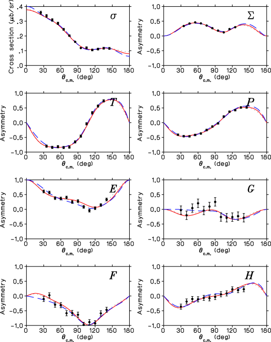
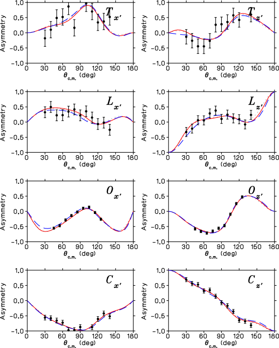
Predictions of the fitted multipole solutions are compared to the data of table 4 in figures 10 and 11 for two beam energies, 1122 and 1421 MeV. The best and worst solutions from the bands of figures 6 and 7, in terms of the /point values of table 6, are shown as the solid (black) and dashed (blue) curves, respectively. The behavior at other energies is very similar. Based on such comparisons with existing published data, the multipole solutions within the bands of figures 6 and 7 are completely indistinguishable. Clearly, despite the presence of 8 polarization observables, the multipoles are still very poorly constrained. For many of the higher multipoles not even the sign is known.
In figures 12 and 13 we compare the , and wave multipoles from existing PWA results (BoGa [28], MAID [23], SAID [26] and JSLT [29]) with the bands of figures 6 and 7, respectively. Here we have rotated all multipoles to our common reference point of a real . (Each set of multipoles has been multiplied by , where is the phase of the multipole of the PWA set.) For the most part, these PWA lie within our experimental solution bands. However, there are a few exceptions at the higher energies, in particular the multipole from Kaon-MAID (black dashed curve in figure 13) and the and multipoles from JSLT (blue solid curves in figure 12). The upper end of our analysis range is near a potentially new . The Kaon-MAID [25] and JSLT groups [29] have associated an enhancement in the cross section near 1.9 GeV with the partial wave, which should resonate in either the or multipoles. However, our model-independent analysis excludes such conclusions, since their solutions lie outside the experimental bands in these partial waves. On the other hand, the BoGa analysis [39] has recently modeled the as a resonance, which should manifest itself in either the or multipoles. The BoGa solution is within the experimental solution bands of figures 12 and 13. (It is also the only PWA analysis that included the CLAS-g1c and GRAAL data sets in fitting their model parameters.) We can conclude that their assignment is consistent with the experimental solution bands, but cannot yet confirm it due to the significant width of these bands.
We have investigated a number of possible ways in which additional data may lead to narrower multipole bands and improved amplitude determination. For the most part, existing data does not extend to extreme angles (near and ), which in general tend to be more sensitive to interfering multipoles of opposite parities. In fact, the best and worst solutions at MeV ( MeV) exhibit a dramatic difference in the predicted unpolarized cross section at – compare the solid (black) and dashed (blue) curves in figure 10. (The extreme angles of the asymmetries are constrained by symmetry to either 0 or , and so contain little additional information.) As a test, we have created mock cross section data at and , centered on the best solutions of table 6 with a statistical error of . When the fits are repeated with these mock points added to the CLAS and GRAAL data sets, variations such as seen in figure 10 disappear, but few of the resulting bands of multipole solutions are improved. While the , and are slightly narrowed at low energies, generally, there is little improvement over the trends seen in figures 6 and 7.
The data in table 4 span a significant range in statistical precision. From preliminary analyses of data from an ongoing generation of new CLAS experiments we can anticipate result on the , , and asymmetries that will have at least an order of magnitude improvement over the GRAAL data set. To simulate the effect of such an improvement, we have arbitrarily reduced the statistical errors on the GRAAL , , and asymmetries by a factor of 3 and repeated the fits. Apart from an increase in , due to undulations in the angular distributions that are now artificially beyond the level of statistical fluctuations, there are no significant changes in any of the multipole bands of figures 6 and 7.
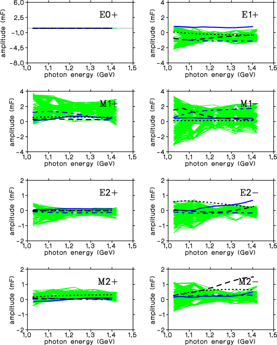
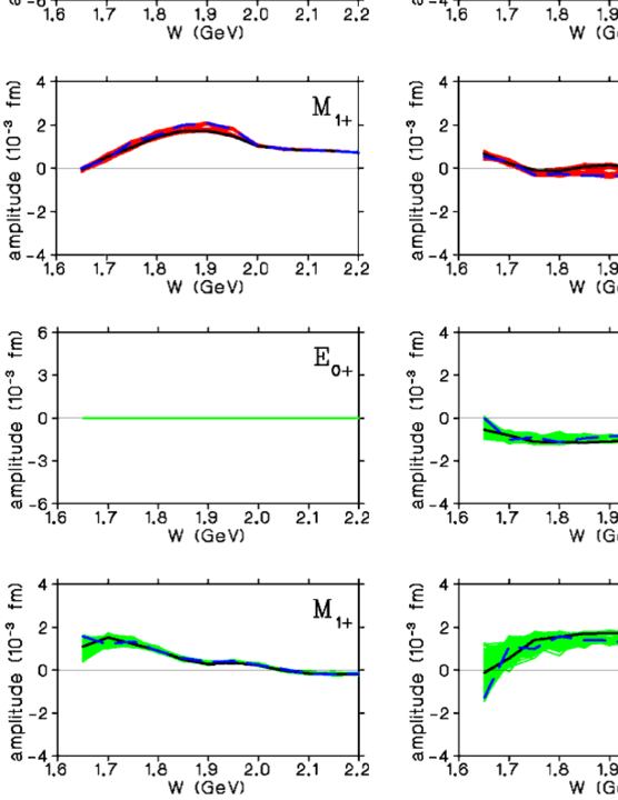
Ongoing analyses of new experiments are expected to yield data on all 16 observables. The potential impact of such an extensive set is simulated in the next section; here we can already study the expected trends by examining the impact that the GRAAL measurements of have made so far. In figure 14 we show the and wave multipoles obtained if the GRAAL data are removed from the fitting procedure. Comparing these results to figures 6 and 7, it is clear that the band has dramatically narrowed with the inclusion of the GRAAL polarization results. Lesser but still significant gains occur in the determination of most of the multipoles. The range of values for the /point within these bands are similar to those of table 6. In figure 15 we show the predictions of the band at 1421 MeV beam energy ( MeV), as represented by the solutions with the minimum and the maximum . Not surprisingly, predictions for the observables where data have been removed from the fit are now wildly varied.

There are several conclusions that can be drawn from this analysis, along with reasons for genuine hope. When the /point is near or even better than 1, solutions differing in the /point by something like 0.2 are not experimentally distinguishable. The existence of bands of multipole solutions, each with small /point, indicates a shallow surface, pitted with many local minima. Certainly the width of the bands evident in figures 6 and 7 precludes using the existing data to hunt for resonances. However, a comparison of figure 14 with figures 6 and 7 indicates the gains resulting from the GRAAL polarization observables are significant, even though the GRAAL errors are substantially larger than most of the CLAS data. CLAS data on all 16 photoproduction observables are now under analysis. The fact that such data have all been accumulated within a single detector is likely to minimize the problems evident in figure 4. Furthermore, with a large number of different observables will come a large number of the Fierz identities, which can be used to constrain and essentially eliminate the effects of systematic scale uncertainties.
10 The potential of complete experiments – studies with mock data
To further investigate the potential impact of measuring a complete set of all 16 observables on the determination of multipole amplitudes, we have created mock data using predictions of the BoGa multipoles, Gaussian-smeared to reflect different levels of uncertainty. Fitting such mock data with the same procedure described in the previous section, i.e., Monte Carlo sampling combined with gradient minimization and a real multipole, leads to the following conclusions.
-
•
With data points at every 10 degrees and with 0.1% errors on each point for every observable, a level of accuracy that will never be achieved at any facility, two minima are always found, one with a /point near 1 and the other substantially larger – e.g., greater than 50. Thus, a unique solution is easily identifiable.
-
•
When the uncertainties on the mock data are increased to 1% on each point every 10 degrees, a few minima appear. Nonetheless, with the exception of the lowest energies, these are still widely spaced in so that in general the true solution can still be identified.
-
•
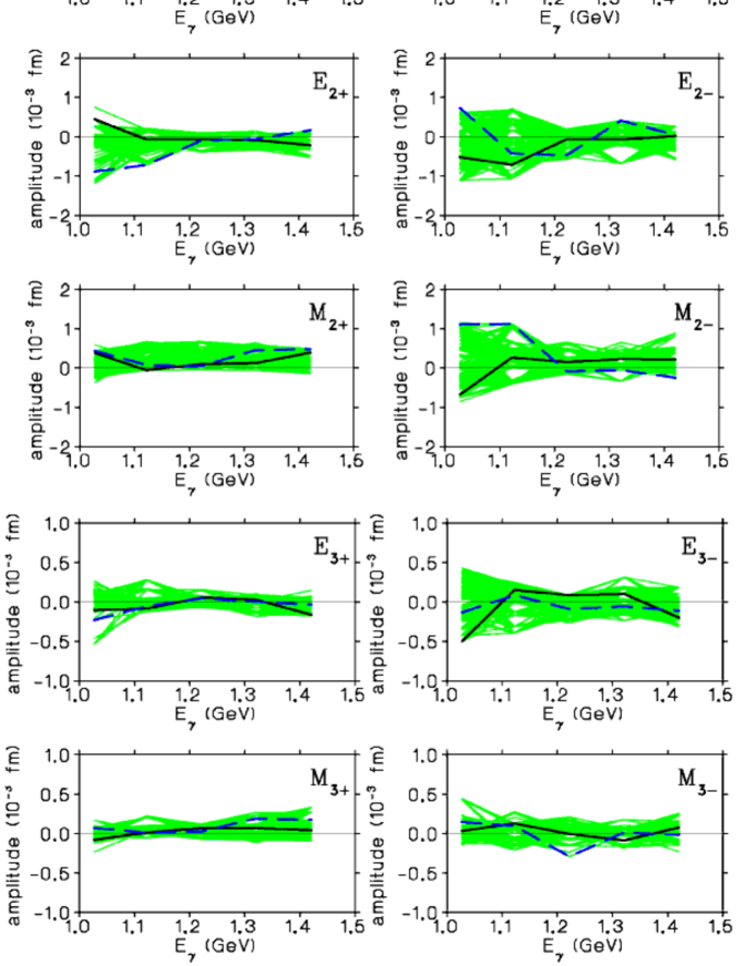
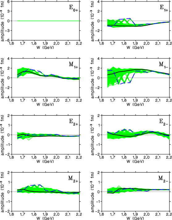
When the uncertainties on the mock data are increased to 5%, bands of indistinguishable solutions from multiple minima begin to appear, although the bands are considerably narrowed from those of figures 6 and 7. As an example, the resulting real and imaginary parts of the to multipoles are shown in figure 16 for the c.m. energy range from 1650 to 2200 MeV. With small errors and bands as narrow as in figure 16, there are typically a few local minima for each energy. However, the positions of such minima depend on the particular statistical distribution of the mock data, due to the complicated structure of the space. To remove this dependence we have repeated the exercise of creating Gaussian smeared mock 5% data and searching for local minima 300 times, with a different random seed to distribute the mock data each time. This is the result plotted in figure 16. It should be noted that a real experiment will not have the luxury of being repeated so many times, if at all, and so fits to the particular statistical distribution of data that is accumulated will have a narrower band width, which will not represent the true uncertainty. Nonetheless, the full uncertainty can readily be determined by simulation.
-
•
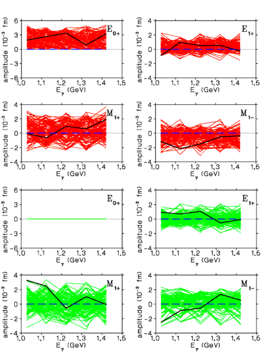
While actual data sets may attain 5% uncertainties on some observables, others will be considerably larger, notably those involving polarized targets which are always significantly shorter than liquid targets. To consider a more realistic collection of data, we have created Gaussian-smeared mock data with a kinematic coverage typical of the CLAS detector at Jefferson Lab, using uncertainties on liquid target measurements taken from the CLAS g1c [20], g8 [32] and g11a [34] data sets, and with polarized target data errors estimated for the g9-FROST running period. As an example, the resulting mock data with expected CLAS uncertainties at MeV are shown in figures 17 and 18. The multipole bands resulting from fits to these mock data are plotted in figures 19 and 20. As with the 5% error study, the Gaussian smearing followed by Monte Carlo and minimization to search for local minima has been repeated 300 times to avoid the dependence on the starting distribution of the data. This had a smaller effect in the resulting multipole bands of figures 19 and 20, since the errors are somewhat larger than the 5% case of figure 16. Compared to figures 6 and 7, the multipole bands of figures 19 and 20 are dramatically narrower. Almost all multipoles are well determined. Some, like the imaginary part of the , remain broad at low energies. But all are well defined above above 1.9 GeV where unobserved states are predicted in various calculations. From extensive studies we attribute this mainly to the larger number of observables rather than to increased statistics on any specific asymmetry. These studies give us confidence in the expectation of a well determined amplitude from complete experiments, such as those from CLAS. This will be a truly significant milestone after over fifty years of photo-production experiments.
11 Summary
It is anticipated that data will soon be available on all 16 pseudoscalar meson photoproduction observables from a new generation of ongoing experiments, certainly for final states and possibly for channels as well. This will significantly reduce the model dependence in the study of excited baryon structure by providing a total amplitude that is experimentally determined to within a phase. Such an experimental amplitude can be utilized at two levels, first as a test to validate total amplitudes associated with different models and second as a starting point that can be analytically continued into the complex plane to search for poles. Here we have laid the ground work for this by assembling a complete and consistent set of equations needed for amplitude reduction from experiment and have demonstrated the first stage of interaction with theoretical models.
In summary, we have used direct numerical evaluations, (32)-(35), to verify the most general analytic form of the cross section, dependent on the three polarization vectors of the beam, target and recoil baryon, including all single, double and triple-polarization terms involving the 16 possible spin-dependent observables (37). (Copies of the associated computer code are available upon request [40].) We have explicitly listed the experimental measurements needed to construct each observable in pseudoscalar meson photoproduction (B) and provided a consistent set of equations relating these quantities to the CGLN amplitudes (58a)-(58p), and from these to electromagnetic multipoles (15)-(18). From a review of some of the more frequently quoted works in this field, we have found that the same symbol for a polarization asymmetry has been used by different authors to refer to different experimental quantities; the magnitudes remain the same across published works, but their signs vary (section 5). For example, the definitions of the six observables , , , , and in the MAID and SAID on-line PWA codes is the negative of that used by BoGa and the present work. This has already lead to confusion in the analysis of recent double-polarization data (figure 3).
We have used the assembled machinery to carry out a multipole analysis of the reaction, free of model assumptions, and examined the impact of recently published measurements on 8 different observables. We have used a combined Monte Carlo sampling of the amplitude space, with gradient minimization, and have found a shallow valley pitted with a very large number of local minima. This results in broad bands of multipole solutions, which are experimentally indistinguishable (figures 6 and 7). Comparing to models that have recently reported a new , we can exclude PWA that incorporate a new since their amplitudes lie outside the model-independent solution bands in the associated multipoles. (These PWA were carried out before most of the data used in our analysis were available.) Recent BoGa analyses have modeled the as a resonance. While their solution lies within our experimental multipole bands, we cannot yet validate it due to the significant width of the bands.
From our studies with published measurements, as well as simulations with mock data, we have seen that clusters of local minima in are often present. With the current collection of results on 8 observables, these minima are completely degenerate and experimentally indistinguishable. In studies with mock data we have seen that this degeneracy can be removed with high precision data on a large number of observables (section 10). As determined in the present analysis, a greater number of different observables tend to be more effective in creating a global minimum than higher precision. We conclude that, while a general solution to the problem of determining an amplitude free of ambiguities may require 8 observables, as has been discussed by CT [2], such requirements assume data of arbitrarily high precision. Experiments with realistically achievable uncertainties will require a significantly larger number. Simulations using mock data with statistics comparable to what is anticipated from the new generation of CLAS experiments reconstruct narrow bands that are quite well defined for almost all multipoles (figures 19 and 20). We expect such results to create a watershed in our understanding of the nucleon spectrum.
Appendix A General expression for the differential cross section with fixed polarizations
We summarize here the derivation of an analytic expression for the differential cross section in pseudoscalar meson photoproduction with general values of the beam, target and recoil polarization. Following the formalism of the spin density matrices described by FTS [11], one can write the general cross section (35) as,
| (58bl) |
(Throughout this appendix the same indices in equations imply taking summation.) Here ; , in which the spin states of the initial and final baryons are quantized in the -direction and the (unit) photon polarization vector is taken to be circularly polarized with the helicity .
The spin density matrix for is given by
| (58bm) | |||||
| (58bn) | |||||
| (58bo) |
where is the Pauli spin vector, as in (24), and is the so-called Stokes vector for the photon polarizations [11]. Note that in the -- coordinate (see figure 2), .
Substituting (58bm)-(58bo) into (58bl), we have
| (58bp) | |||||
Noting that where , we can further expand the above equation as
| (58bq) | |||||
In the last step we have introduced
| (58br) | |||||
| (58bs) | |||||
| (58bt) | |||||
| (58bu) | |||||
| (58bv) | |||||
| (58bw) | |||||
| (58bx) |
In (58bq)-(58bx) the Pauli matrices that are combined in products with beam and target polarizations are defined in reference to the unprimed coordinates of figure 2 with the beam along , so that
However, the Pauli matrices appearing in products with the recoil polarization vector are defined in reference to the primed coordinates of figure 2 with the meson momentum along , so that
[If the unprimed coordinates were also used to expand , then one would obtain a corresponding set of unprimed observables that are related via equation (38).]
We note that , , , , , and are exactly the same as those defined in [11]. The term was not included in [11], which did not consider the triple polarization case. Each component in (58br)-(58bx) can be related with 16 observables defined in tables 7-10 of B:
| (58by) |
| (58bz) |
| (58ca) |
| (58cb) |
| (58cc) |
Here, all other components not explicitly shown are identically zero, due to symmetry constraints.
Finally, we also note that the spin density matrices (58bm)-(58bo) can be expressed as
| (58cd) | |||||
| (58ce) | |||||
| (58cf) |
Here is the probability of observing particle polarized in the direction; is the Stokes vector specified by the unit photon polarization vector ; is a unit photon polarization vector perpendicular to for linearly polarized photons, while and express two different helicity states for circularly polarized photons. The non-unit polarization vectors can be expressed with the unit polarization vectors as , , and . Substituting (58cd)-(58cf) into (58bl), one obtain the relation between the general cross sections with unit and non-unit polarization vectors (35).
Appendix B Constructing observables from measurements
We tabulate here the pairs of measurements needed to construct each of the 16 transverse photoproduction observables in terms of the polarization orientation angles of figure 2. The photon beam is characterized either by its helicity, for circular polarization, or by for linear polarization. Assuming 100% polarizations, each observable is determined by a pair of measurements, each denoted as ; “unp” indicates the need to average over the initial spin states of the target and/or beam, and to sum over the final spin states of the recoil baryon. For observables involving only beam and/or target polarizations, and . For observables involving the final state recoil polarization, and .
-
, , , Beam Target Recoil Observable unp unp unp unp unp unp - unp unp unp unp - 0 unp unp unp unp unp unp unp unp unp unp unp unp unp unp unp unp unp unp unp unp
-
- Beam Target Recoil Observable - 0 unp unp - 0 0 unp unp - 0 unp unp - 0 unp unp - 0 0 unp unp - 0 unp unp - 0 0 unp unp - 0 0 unp unp - 0 unp unp - 0 unp unp - 0 unp unp - unp unp - 0 unp unp - 0 unp unp - 0 unp unp - unp unp
-
- Beam Target Recoil Observable - unp unp 0 - unp unp 0 - unp unp 0 - unp unp 0 - unp unp 0 - unp unp 0 - unp unp 0 - unp unp 0 - unp unp 0 - unp unp 0 - unp unp 0 - unp unp 0 - unp unp 0 - unp unp 0 - unp unp 0 - unp unp 0
-
- Beam Target Recoil Observable unp unp 0 0 0 unp unp 0 0 unp unp 0 0 0 unp unp 0 0 0 unp unp 0 0 0 unp unp 0 0 unp unp 0 0 0 unp unp 0 0 0 unp unp 0 0 unp unp 0 unp unp 0 0 unp unp 0 0 unp unp 0 0 unp unp 0 unp unp 0 0 unp unp 0 0
Appendix C The Fierz identities
We list here the Fierz identities relating asymmetries, with signs consistent with the definition of observables in B and with the form of the general cross sections in equation (37). The equation numbering sequence in C.1-C.3 is that of Chiang and Tabakin [2]. Compared to the results given in [2], our equation (L.0) differs by a factor and the remaining expressions have different signs in all but (L.1), (L.4)-(L.6), (Q.r), (Q.bt.3), (Q.tr.1), (Q.tr.2); needless to say, the six Squared relations are the same. Sign changes in eight of the equations can be attributed to the different definition for the asymmetry used by Fasano, Tabakin and Saghai [11], to which Chiang and Tabakin refer.
C.1 Linear-quadratic relations
| (L.0) | |||||
| (L.TR) |
| (L.BR) |
| (L.BT) |
| (L.1) |
| (L.2) |
| (L.3) |
| (L.4) |
| (L.5) |
| (L.6) |
| (L.7) |
| (L.8) |
| (L.9) |
| (L.10) |
| (L.11) |
| (L.12) |
C.2 Quadratic relations
| (Q.b) |
| (Q.t) |
| (Q.r) |
| (Q.bt.1) |
| (Q.bt.2) |
| (Q.bt.3) |
| (Q.bt.4) |
| (Q.br.1) |
| (Q.br.2) |
| (Q.br.3) |
| (Q.br.4) |
| (Q.tr.1) |
| (Q.tr.2) |
| (Q.tr.3) |
| (Q.tr.4) |
C.3 Squared relations
| (S.bt) |
| (S.br) |
| (S.tr) |
| (S.b) |
| (S.t) |
| (S.r) |
C.4 ARS-squared relations
Here we include a set of squared relations discussed in Artru, Richard and Soffer (ARS) [31]. These can be derived from combinations of relations in the preceding sections. For example, the first, (ARS.S.bt), can be obtained by combining (S.bt) and (L.BT). Our relations differ in sign from ARS in those terms involving , and , and as a result there are sign differences in (ARS.S.bt), (ARS.S.br) and (ARS.btr1).
| (ARS.S.bt) |
| (ARS.S.br) |
| (ARS.S.tr) |
| (ARS.btr1) |
| (ARS.btr2) |
Appendix D Born amplitudes for
In this Appendix, we summarize the Born amplitudes for in the center of mass energy (, ), which are used to fix high partial waves () in the multipole analyses presented in section 9. We consider the following Born terms for [see the paragraph including (6) for the description of ]:
| (D.1) |
where
| (D.2) | |||||
| (D.3) | |||||
| (D.4) | |||||
| (D.5) | |||||
| (D.6) | |||||
| (D.7) | |||||
with and
| (D.8) | |||||
| (D.9) | |||||
| (D.10) |
Also, we have introduced the dipole form factors for the hadronic vertex defined as
| (D.11) |
References
References
- [1] Chew G R, Goldberger M L, Low F E and Nambu Y 1957 Phys. Rev. 105 1345
- [2] Chiang W T and Tabakin F 1997 Phys. Rev. C 55 2054
- [3] The g9-FROST series of experiments, URL http://clasweb.jlab.org/shift/g9/ .
- [4] The g14-HDice experiment, URL http://www.jlab.org/exp_prog/proposals/06/PR-06-101.pdf
- [5] Lleres A et al. 2007 Eur. Phys. J. A 31 79
- [6] Lleres A et al. (GRAAL Collaboration) 2009 Eur. Phys. J. A 39 149
- [7] Barker I S, Donnachie A and Storrow J K 1975 Nucl. Phys. B95 347
- [8] Donnachie A and Shaw G 1966 Appl. Phys. 37 333
- [9] Donnachie A (edited by Bishop E H S) 1972 Pure and Applied Physics vol 25-V (Academic Press, New York) p 1
- [10] Adelseck R A and Saghai B 1990 Phys. Rev. C 42 108
- [11] Fasano C G, Tabakin F and Saghai B 1992 Phys. Rev. C 46 2430
- [12] Drechsel D and Tiator L 1992 J. Phys. G 18 449
- [13] Knöchlein G, Drechsel D and Tiator L 1995 Z. Phys. A 352 327
- [14] Jackson J D 1975 Classical Electrodynamics (John Wiley & Sons, New York)
- [15] Bjorken J D and Drell S D 1964 Relativistic Quantum Mechanics (McGraw-Hill, New York)
- [16] Jacob M and Wick G C 1959 Ann. Phys. 7 404; Jacob M and Wick G C 2000 Ann. Phys. 281 774
- [17] Brink D M and Satchler G R 1968 Angular Momentum (Oxford University Press, Oxford)
- [18] Worden R 1972 Nucl. Phys. B37 253
- [19] Hoblit S et al. (LEGS-Spin Collaboration) 2009 Phys. Rev. Lett. 102 172002, and references therein.
- [20] Bradford R K et al. (CLAS Collaboration) 2007 Phys. Rev. C 75 035205
- [21] Lee T D and Yang C N 1957 Phys. Rev. 108 1645
- [22] K. Nakamura et al. (Particle Data Group) 2010 J. Phys. G 37 075021
- [23] MAID and Kaon-MAID isobar models of meson production, URL http://wwwkph.kph.uni-mainz.de/MAID/.
- [24] Drechsel D, Kamalov S S and Tiator L 2007 Eur. Phys. J. A 34 69
- [25] Mart T and Bennhold C 1999 Phys. Rev. C 61 012201
- [26] SAID partial wave analysis facility, URL http://gwdac.phys.gwu.edu/.
- [27] Arndt R A, Briscoe W J, Strakovsky I I and Workman R L 2002 Phys. Rev. C 66 055213
- [28] Anisovich A V, Klempt E, Nikonov V A, Matveev M A, Sarantsev A V and Thoma U 2010 Eur. Phys. J. A 44 203; Bonn-Gatchina Partial Wave Analysis, URL http://pwa.hiskp.uni-bonn.de/
- [29] Juliá-Díaz B, Saghai B, Lee T S H and Tabakin F 2006 Phys. Rev. C 73 055204
- [30] Artru X, Richard J M and Soffer J 2007 Phys. Rev. C 75 024002
- [31] Artru X, Elchikh M, Richard J M, Soffer J and Teryaev O V 2009 Phys. Rep. 470 1
- [32] Ireland D (private communication)
- [33] Glander K K et al. (SAPHIR Collaboration) 2004 Eur. Phys. J. A 19 2
- [34] McCracken M E et al. (CLAS Collaboration) 2010 Phys. Rev. C 81 025201
- [35] Bradford R K et al. (CLAS Collaboration) 2006 Phys. Rev. C 73 035202
- [36] Zegers R G T et al. (LEPS Collaboration) 2003 Phys. Rev. Lett. 91 92001
- [37] Blanpied G et al. (LEGS Collaboration) 2001 Phys. Rev. C 64 25203
- [38] Bowcock J E and Burkhardt H 1975 Rep. Prog. Phys. 38 1099
- [39] Anisovich A V, Kleber V, Klempt E, Nikonov V A, Sarantsev A V, and Thoma U 2007 Eur. Phys. J. A 34 243
- [40] H. Kamano, hkamano@jlab.org
- [41] Juliá-Díaz B, Lee T S H, Matsuyama A and Sato T 2007 Phys. Rev. C 76 065201
- [42] Oh Y, Nakayama K and Lee T S H 2006 Phys. Rep. 423 49