On the Foundations of Adversarial Single-Class Classification

Abstract

Motivated by authentication, intrusion and spam detection applications we consider single-class classification (SCC) as a two-person game between the learner and an adversary. In this game the learner has a sample from a target distribution and the goal is to construct a classifier capable of distinguishing observations from the target distribution from observations emitted from an unknown other distribution. The ideal SCC classifier must guarantee a given tolerance for the false-positive error (false alarm rate) while minimizing the false negative error (intruder pass rate). Viewing SCC as a two-person zero-sum game we identify both deterministic and randomized optimal classification strategies for different game variants. We demonstrate that randomized classification can provide a significant advantage. In the deterministic setting we show how to reduce SCC to two-class classification where in the two-class problem the other class is a synthetically generated distribution. We provide an efficient and practical algorithm for constructing and solving the two class problem. The algorithm distinguishes low density regions of the target distribution and is shown to be consistent.

1 Introduction

In Single-Class Classification (SCC) the learner observes a training set of sampled instances from one target distribution. The goal is to create a classifier that can distinguish instances emitted from distributions other than the target distribution and unknown to the learner during training. This SCC problem can model many applications such as intrusion, fault and novelty detection. For example, in an instance of an intrusion detection problem <see e.g.,¿NisensonYEM03, the goal is to create a classifier that can distinguish ‘legal’ users from intruders based on behaviometric or biometric patterns. This classifier can then be used to guard against illegal attempts to gain access into protected systems or regions.

Single-class classification (also termed one-class classification) has been receiving considerable research attention in the machine learning and pattern recognition communities. For example, only the survey papers Markou  Singh (20031, 20032); Hodge  Austin (2004) cite, altogether, over 100 SCC papers. Most SCC works implicitly assume that a good solution can be achieved by identifying low density regions of the target distribution and then, the objective is to reject sub-domains of low density. Thus, the main consideration in previous SCC studies has been statistical: how can a prescribed false positive rate be guaranteed given a finite sample from the target distribution.

The proposed approaches are typically generative or discriminative. Generative solutions range from full density estimation Bishop (1994), to partial density estimation such as quantile estimation G. Lanckriet . (2002), level set estimation Ben-David  Lindenbaum (1995); Steinwart . (2005) or local density estimation Breunig . (2000). In discriminative methods one attempts to generate a decision boundary appropriately enclosing the high density regions of the training set Yu (2005). In addition to such constructions, there are many empirical studies of the proposed solutions. Nevertheless, it appears that the area suffers from a lack of theoretical contributions and principled (empirical) comparative studies of the proposed solutions.

Motivated mainly by intrusion detection applications, in this paper we examine the SCC problem from an adversarial viewpoint where an adversary selects the attacking distribution. We begin by abstracting away the statistical estimation component of the problem by considering a setting where the learner has a very large sample from the target distribution. This setting is modeled by assuming that the learning algorithm has precise knowledge of the target distribution. While this assumption would render almost the entire body of SCC literature superfluous, it turns out that a significant and non-trivial decision-theoretic component of the adversarial SCC problem remains – one that has so far been overlooked. For a discrete version of the SCC problem we provide an in depth analysis of adversarial SCC and identify optimal strategies for variants of the problem depending on whether or not the learner can play a randomized strategy and on various constraints on the adversary. As a consequence of this analysis, it can be demonstrated that a randomized learner strategy can be superior on average to standard deterministic classification. For an infinitely continuous version of this game we provide a simple and consistent SCC algorithm that implements the standard low-density rejection by reducing the SCC problem to two-class soft classification.

The body of this paper contains the principal results that are simpler to present. The appendices contain some of the more technical proofs. to the presented results. An earlier version of this work containing a subset of the results was presented at NIPS El-Yaniv  Nisenson (2006). Extensions to this work can be found in the thesis of Nisenson (2010).

2 Problem Formulation

We define the adversarial single-class classification (SCC) problem as a two-person zero-sum game between the learner and an adversary. The learner receives a training sample of examples from a target distribution $P$ defined over some space $\Omega$. On the basis of this training sample, the learner should select a rejection function $r:\Omega\to[0,1]$, where for each $\omega\in\Omega$, $r(\omega)$ is the probability with which the learner will reject $\omega$. On the basis of any knowledge of $P$ and/or $r(\cdot)$, the adversary selects an attacking distribution $Q$, defined over $\Omega$. Then, a new example is drawn from $\gamma P+(1-\gamma)Q$, where $0<\gamma<1$, is a switching probability unknown to the learner.

The rejection rate of the learner, using a rejection function $r$, with respect to any distribution $D$ (over $\Omega$), is $\rho(r,D){\stackrel{{\scriptstyle\vartriangle}}{{=}}}{\mathbf{E}}_{D}\{r(\omega)\}$. The two main quantities of interest here are the false positive rate (type I error) $\rho(r,P)$, and the false negative rate (type II error) $1-\rho(r,Q)$. Before the start of the game, the learner receives a tolerance parameter $0<\delta<1$, giving the maximally allowed false positive rate. A rejection function $r(\cdot)$ is valid if its false positive rate satisfies the constraint $\rho(r,P)\leq\delta$. A valid rejection function (strategy) is optimal if it guarantees the smallest false negative rate amongst all valid strategies.

This setting conveniently models various SCC applications and in particular, intrusion detection problems. For example, considering biometric authentication, the false alarm rate $\rho(r,P)$ is the rejection (failed authentication) rate of the legal users and $\rho(r,Q)$ is the rejection rate of intruders, which should be maximized.

Remark 1.

Clearly, a dual SCC problem can be formulated where a sufficiently high intruder rejection rate must be guaranteed and the false alarm rate should be minimized. We briefly discuss this dual problem and its relation to the “primal” in Section 8. Other types of SCC problems can be considered where the loss is a function of the type I and type II errors. For example, one may be interested in minimizing a convex combination of these errors. Any such loss function can be handled using our definition and searching for the $\delta$ for which the SCC solution optimizes the desired loss function.

Our analysis begins by focusing on the Bayes decision theoretic version of the SCC problem in which the learner knows the target distribution $P$ precisely. The problem is thus viewed as a two-person zero sum game where the payoff to the learner is $\rho(r,Q)$. The set ${\mathcal{R}}_{\delta}(P){\stackrel{{\scriptstyle\vartriangle}}{{=}}}\{r:\rho(r,P)\leq\delta\}$ of valid rejection functions is the learner’s strategy space. We denote by ${\mathcal{Q}}$ be the strategy space of the adversary, consisting of all allowable distributions $Q$ that can be selected by the adversary.

We are concerned with optimal learner strategies for game variants distinguished by the adversary’s knowledge of the learner’s strategy, $P$ and/or of $\delta$ and by other limitations on ${\mathcal{Q}}$. We also distinguish a special type of this game, which we call the hard setting in which the learner is constrained to employ only deterministic reject functions; that is, $r:\Omega\to\{0,1\}$, and such rejection functions are termed “hard.” The more general game defined above (with “soft” functions) is called the soft setting. As far as we know, only the hard setting has been considered in the SCC literature thus far. The reason for considering soft rejection functions is that they can achieve significant advantage in terms of type II error reduction. Later on in Section 6.2.1 we numerically demonstrate such error reductions.

For any rejection function, the learner can reduce the type II error by rejecting more (i.e., by increasing $r(\cdot)$). Therefore, in the soft setting for an optimal $r(\cdot)$ we must have $\rho(r,P)=\delta$ (rather than $\rho(r,P)\leq\delta$). It follows that the switching parameter $\gamma$ is immaterial to the selection of an optimal strategy.

Given an adversary strategy space, ${\mathcal{Q}}$, we define the set ${{\mathcal{R}}_{\delta}^{*}}(P)$ of optimal valid rejection functions as ${{\mathcal{R}}_{\delta}^{*}}{\stackrel{{\scriptstyle\vartriangle}}{{=}}}\{r\in{\mathcal{R}}_{\delta}(P)\ :\min_{Q\in{\mathcal{Q}}}\rho(r,Q)=\max_{r^{\prime}\in{\mathcal{R}}_{\delta}(P)}\min_{Q^{\prime}\in{\mathcal{Q}}}\rho(r^{\prime},Q^{\prime})\}$. We note that ${{\mathcal{R}}_{\delta}^{*}}$ is never empty in the cases we consider.

3 Related Work

One-Class Classification is often given different names, depending on the desired use. For example, other common names include outlier detection, fault detection and novelty detection. Historically, one of the earliest works is due to Grubbs69 who considered in-sample outlier detection. Grubbs calculates a cut-off statistic for determining outliers in the 1-dimensional Gaussian case at the 5%, 2.5% and 1% significance levels within samples of various sizes. Minter75 appears to be the first to use the term “single-class classification”. Minter starts from a fairly standard two-class approach, assuming that there is a class of interest (class 1) and a class of “others” (class $\emptyset$). Given the switching parameter $\gamma$ (which is the a priori probability of class 1), Minter gives the rule to accept a point $x$ iff $\gamma\Pr\{x|1\}\geq(1-\gamma)\Pr\{x|\emptyset\}$, which is equivalent to $\gamma\Pr\{x|1\}\geq\frac{1}{2}\Pr\{x\}$. It is assumed that both $\gamma$ and $\Pr\{x\}$ are known or can be estimated from historical data, leaving the problem of estimating $\Pr\{x|1\}$ from the given sample. While, technically, only a sample from the class of interest is given, the additional assumptions make this a modified form of a two-class problem. These are the earliest explicit works we have found. Note that statisticians have long been considering the two-sample problem, which is similar but perhaps simpler. One can view the SCC problem as an extremely unbalanced instance of the two-sample problem that prevents using the standard statistical hypothesis testing techniques.

Since virtually all prior works on SCC that we have encountered deal with how to approximate a low-density rejection strategy given a set, $\{x_{1},\ldots,x_{n}\}$, of training points, sampled from the class of interest, we will focus our review here on such methods.

We begin with discussing support, quantile and level-set estimation. Support estimation aims to estimate the support of a density $p$. In terms of outlier detection, the goal is clear: a point falling outside the estimated support is taken to be an outlier. One of the simpler methods, analyzed by DevroyeWise80, is to estimate the support as $\hat{S}_{n}=\bigcup_{i=1}^{n}B(x_{i},\epsilon_{n})$, where $B(x,a)$ is a closed ball centered at $x$ with radius $a$ (i.e. $||x^{\prime}-x||\leq a$, for some norm $||\cdot||$), and $\epsilon_{n}$ is a (vanishing) sequence of smoothing parameters. In quantile estimation, the goal is to find a set $U(\beta)$ such that $\lambda(U(\beta))=\inf_{S}\{\lambda(S):P(S)>\beta\}$, where $\lambda$ is a real valued function. For our purposes, we take $\lambda$ as the Lebesgue measure, in which case the problem is also called minimum volume estimation. When $\beta=0$ this becomes support estimation, and when $\beta=1-\delta$ this problem is the same as low-density rejection. In level-set estimation, the goal is to approximate the set ${\mathcal{L}}(t)=\{x:p(x)>t\}$ (or alternatively as $\{x:p(x)\geq t\}$). Of course, level-set estimation can be used for support estimation by taking $t=0$ or by taking $t=t_{n}$ as a sequence which approaches zero <see¿Cuevas97. Clearly, level-set estimation approximates the low-density rejection strategy when $P({\mathcal{L}}(t))=1-\delta$. A significant amount of prior SCC works have focused on minimum volume and level-set estimation. We distinguish between explicit and implicit methods, where explicit methods try to directly solve one of the problems, and implicit methods which use a heuristic which may or may not give the desired result. We note that whether the method is explicit or implicit is not necessarily an indicator of whether the underlying model is generative or discriminative, although there is a clear tendency for explicit methods to be generative. Transformations from the one-class setting to the two-class setting tend to be implicit and discriminative. We will consider minimum volume estimation approaches first and then look at various level-set estimation results. Finally we will examine other results, including transformations to the two-class setting.

Minimum volume estimation has been a favored approach at solving the SCC problem in the literature. This perhaps is due to two works which reused the popular Support Vector Machine <SVM, see¿Vap98 from two-class classification problems. The earlier work D. Tax  Duin (1999) sought to fit the sample data inside a sphere of minimal radius, a solution they called the Support-Vector Data Description (SVDD). Specifically, given a sphere with center $a$ and radius $R$, the error function to be minimized is $R^{2}+C\sum_{i}\xi_{i}$, under the constraints $(x_{i}-a)^{T}(x_{i}-a)\leq R^{2}+\xi_{i}$, where $C$ is a regularization term which relates to the type I error. Outliers in the sample data would lie on, or outside the sphere (and have $\xi_{i}>0$). The kernel trick was then employed to allow for solving the problem in a higher dimensional feature space. They note that polynomial kernels do not result in small volumes in the input space, as points distant from the origin tend to have high error values. They found that Gaussian kernels worked well. The type I error can be estimated from the number of support vectors divided by the sample size, $n$, where the support vectors are the points lying on the sphere (i.e. they define the sphere’s boundary). Changing the regularization parameter $C$, or the bandwidth parameter of the Gaussian kernel, can be used to control the trade-off between the volume of the sphere and the number of support vectors. In a follow up work, TaxD01 show how samples from a uniform distribution can be used to optimize for both parameters simultaneously. The second work Schölkopf . (2001) introduced what is commonly called the One-Class Support Vector Machine (OC-SVM). The technique used is that of a standard two-class SVM where the second class is the origin (in feature space). In other words, a hyper-plane is sought which maximizes the soft-margin between the origin and the sample points. Points lying on the “wrong” side of the hyper-plane are outliers. The kernel trick can also be employed for OC-SVM. Schölkopf et. al show that for kernels $k(x,y)$ that depend only on $x-y$, such as the Gaussian kernel, the solutions found by OC-SVM and SVDD are identical. They further showed that the value $\nu=\frac{1}{nC}$, where $C$ is the regularization parameter in the SVM equation, is an upper bound on the number of outliers, a lower bound on the number of support vectors, and that for probability measures $P$ without discrete components, asymptotically the number of outliers and support vectors are equal, in probability. Vert06 correctly point out that while OC-SVM can guarantee the type I error, no guarantees are made regarding consistency of the result (i.e., whether the result converges to a region of minimum volume). This same point is valid for SVDD as well. Indeed, the poor performance of SVDD using polynomial kernels is sufficient proof that the minimum volume set (in the original feature space) is not found. Thus, both of these approaches are implicit, as they do not explicitly solve for the minimum volume set. Similar results for the Minimax Probability Machine (where the type I error is bounded but the resulting set does not necessarily have the minimum volume) are provided by Lanckriet et. al GRG. Lanckriet . (2002); G. Lanckriet . (2002). ScottNowak06 overcome these limitations where they use Empirical Risk Minimization to prove consistency (in a distribution free manner) and convergence rates of $\left(\frac{\log n}{n}\right)^{\frac{1}{d}}$ using Structural Risk Minimization for trees (these results aren’t distribution free; specifically there is a requirement which can be satisfied if $p$ has no plateaus). Scott07 expands on this analysis, which served as the basis for the 2-class SVM approach used in Davenport . (2006), where the second class is the uniform distribution. The results significantly outperformed those of OC-SVM (i.e. a significantly smaller volume was found for approximately the same type I error).

We now turn our attention to level-set estimation. Let ${\mathcal{L}}_{n}(t)$ be the estimation of ${\mathcal{L}}(t)$ given the $n$ sample points. One of the most common error measures is $\lambda({\mathcal{L}}(t)\mathop{\Delta}{\mathcal{L}}_{n}(t))$, where $\lambda$ is the Lebesgue measure and $\mathop{\Delta}$ is the symmetric difference (i.e. $A\mathop{\Delta}B=(A\setminus B)\bigcup(B\setminus A)$). Another common measure is $H_{P}({\mathcal{L}}(t),t)-H_{P}({\mathcal{L}}_{n}(t),t)$, where $H_{P}(S,t)=P(S)-t\lambda(S)$ is the excess mass of $S$. Both of these measures are non-negative and equal to zero at the optimal solution. Much of the prior work which explicitly solves the level-set estimation problem shows consistency by proving that as $n$ goes to infinity, one of these two measures goes to zero. Most recent work focuses on calculating convergence rates under various conditions on the density $p$. One of the most common techniques for level-set estimation is the plug-in estimate where ${\mathcal{L}}_{n}(t)=\{x:\hat{p}_{n}(x)>t\}$, for a density estimate $\hat{p}_{n}$ of $p$. The kernel density estimate Parzen (1962) is most often used. For a thorough analysis of the plug-in estimate (in terms of consistency and convergence rates) see Cuevas97,Cadre97,Rigollet08. Interestingly, the SCC community appears to have been inclined to pursue alternate and novel approaches over the straight-forward use of the kernel density estimate as part of the plug-in estimator. It must be stressed that these approaches have largely been implicit, in the sense that they are based on either a heuristic or some other approximation, and consistency is not proven. For example, BreunigKNS00 develop a measure they call the Local Outlier Factor (LOF). LOF is calculated based on a smoothed k-nearest-neighbor distance, where the LOF is calculated as an average ratio of these distances between the neighbors of a point and the point itself. In other words, the LOF is calculated so that objects “deep within a cluster” will have a LOF of approximately 1, while objects near edges of clusters or far from other points will have large values. This seems to be a heuristic way of estimating $f(p)$ where $f$ is hoped to be a monotonically decreasing function. Hempstalk2008 use the plug-in estimate approach where they use a rather different way of establishing $\hat{p}_{n}$. Using Minter’s notation from above, they generate an artificial distribution for class $\emptyset$, and then it follows from Bayes Theorem that:

$$\Pr\{x|1\}=\frac{\Pr\{\emptyset\}\Pr\{1|x\}}{\Pr\{1\}\Pr\{\emptyset|x\}}\Pr\{x|\emptyset\}.$$

Since the artificial distribution is known, and the prior can be controlled, $\Pr\{x|1\}$ can be estimated from $\Pr\{1|x\}$, which is estimated using class-probability estimation techniques, specifically bagged trees with Laplacian smoothing. In practice, they use a density estimate of $p$ to establish the density for the artificial set. While the technique is certainly interesting, it would be of great interest to see if consistency or convergence rates could be proven. Vert06 demonstrated that one need not estimate the density directly in order to determine the level-set. They prove that an SVM, with a convex loss function and Gaussian kernel with a “well-calibrated bandwidth $\sigma$,” can produce an estimate ${\mathcal{L}}_{n}(t)$, such that $\lim_{n\to\infty}H_{P}({\mathcal{L}}(t),t)-H_{P}({\mathcal{L}}_{n}(t),t)=0$, in probability. SteinwartHS04 provide convergence rates when using L1-SVM for the error measure $\mu({\mathcal{L}}(t)\mathop{\Delta}{\mathcal{L}}_{n}(t))$, where $\mu$ is a reference probability distribution.

Finally, we consider other works, starting with transformations to the two-class setting. All of these approaches rely on the creation of a second class in the vicinity of the target class. Examples of this are Bánhalmi . (2007) where SVM is used to separate between the two classes, and Curry  Heywood (2009), where genetic programming is used and the fitness function accounts for overlap between the two classes. Other works, such as Rätsch . (2002), look at how boosting can be applied in the one-class setting. A recent and interesting work is by Juszczak_09_spanning_tree, which uses the premise that the target class should largely be continuous; in other words, if two points belong to the target class, there should be a path from one to the other. For points which are very close to each other, we may expect this to be a straight line. They propose building a minimum spanning tree covering the data, and test membership to the target class by testing the distance of a point to the tree. Since the continuity assumption may be violated for points in different clusters, they allow for the removal of edges in the tree, where longer edges are better candidates for removal. They also allow for a form of dimensionality reduction by removing the shortest paths in the tree. The approach has very good performance on the tested data sets, and it would be of great interest to see if the authors can develop consistency or other theoretical results for it.

4 An Informal Look - an Investment/ROI Analogy

To gain some insight into the one-class classification setting, we now describe an analogous investment game. The learner is given an amount of money to invest, $\delta$. There are $N$ assets which can be invested in, with a cost of $p_{i}$ to invest in asset $i$. For each asset $i$, the learner purchases an amount $r(i)\in[0,1]$ (i.e., from none to all of an asset) and then sells it at a price $q_{i}$, determined by the adversary. Any monies not invested are lost. Since the initial wealth is $\delta$, the allocation strategy $r(\cdot)$ must satisfy $\sum_{i}r(i)p_{i}\leq\delta$. The overall return to be maximized is $\sum_{i}r(i)q_{i}$.

Clearly, the Return-On-Investment (ROI) for asset $i$ is $\frac{q_{i}}{p_{i}}$, and thus the learner should invest in assets which have the highest ROI (where free assets are taken to have infinite ROI). In the SCC setting, the fact that the learner must select the investment strategy, $r(\cdot)$, before the adversary determines the selling prices, clearly makes this a difficult proposition. Had we reversed the order, and the adversary were to determine the selling prices first, we would have a two-class classification problem (i.e., the learner, with full knowledge of both classes, is to minimize type II error subject to a maximum type I error). In this case, the learner’s optimal investment strategy would be clear:

The learner shouldn’t invest in an asset $k$, unless all assets with a higher ROI than $k$ have already been purchased.

Note that while this strategy applies to the soft setting ($r(i)\in[0,1]$), the optimal solution is very nearly identical to that of the hard solution ($r(i)\in\{0,1\}$), with the only difference being that any left over money is invested. How does this investment strategy translate from the two-class classification setting to our original one-class classification setting, where the learner must invest without knowing the ROI values? Clearly, if the adversary’s strategy space has some inherent constraints on the relative ROI of assets, then the learner could take advantage of them. For example, in the simplest case, if the adversary’s strategy space enforces an ordering on the ROI values, for example $j<k\Rightarrow\frac{q_{j}}{p_{j}}<\frac{q_{k}}{p_{k}}$, then the learner can invest optimally without knowing $Q$. However, the less the adversary’s strategy space constrains the relative ROI of assets, the more difficult the learner’s task is. We would intuitively expect that, in the face of an adversary determined to minimize the learner’s return, that less constraints on the adversary would force the learner to diversify his investment. In the extreme case of no constraints at all on the adversary, the learner should purchase the same amount of every non-free asset. We also note that the more the learner diversifies, the “further” his investment strategy becomes relative to the optimal two-class strategy (in accordance to known ROI values).

5 On the Optimality of Monotone and Low-Density Rejection Functions

The vast majority of the literature on SCC deals with various techniques for implementing the Low-Density Rejection Strategy (LDRS). This raises the question of whether such a strategy is optimal or not, and under what conditions may it be reasonable to use such a strategy. Since we are interested in adversarial applications, worst-case performance is a natural measure for us to consider. For example, if one considers an authentication system every attempt to gain access results in either access being granted or an alarm being fired. From a worst-case perspective, we should expect a sophisticated intruder to be capable of spying upon legitimate use of the system for some period of time and seeing what events or patterns should provide access. Thus, it is more likely that the intruder will attempt to enter a highly probable event in order to gain access, rather than a low-probability event. In fact, the intruder’s distribution could be even more concentrated on the highly-probable events than the user’s!

Viewed in this perspective, it is not at all clear at the outset that the standard LDRS approach to SCC is the best for adversarial applications. By constraining the adversary’s strategy space to one where all of the distributions are tightly concentrated on the highly-probably events under $P$, low-density-rejection may not be an optimal strategy for the learner. In the extreme case where the adversary always plays the most probable event under $P$, the adversary would always be able to gain access if the learner plays the low-density-rejection strategy, while potentially the learner could completely deny the adversary access if $\delta$ is greater than the probability for that event. Clearly, the nature of the constraints placed on the adversary is critical not only in terms of whether LDRS is optimal, but also in terms of the error that is achievable (both by LDRS and by other strategies). Here we address the former issue, which we feel is of particular relevance considering the large body of existing work which examines approximating low-density rejection functions that can be leveraged in solving practical problems, and leave the latter for future research.

The partially good news is that low-density rejection is worst-case optimal if the learner is confined to “hard” decisions and when the adversary is strong enough in the sense that her strategy space is sufficiently large as shown in Theorem 10. However, as we demonstrate in Section 6, LDRS is inferior in general to the optimal soft strategy. Thus, by playing a randomized strategy, a very significant gain can be achieved.

In this section, we assume a finite support of size $N$; that is, $\Omega=\{1,\ldots,N\}$ and $P{\stackrel{{\scriptstyle\vartriangle}}{{=}}}\{p_{1},\ldots,p_{N}\}$ and $Q{\stackrel{{\scriptstyle\vartriangle}}{{=}}}\{q_{1},\ldots,q_{N}\}$ are probability mass functions. Note that this assumption still leaves us with an infinite game because the learner’s pure strategy space, ${\mathcal{R}}_{\delta}(P)$, is infinite. Extensions to infinite support ($N\to\infty$) for many of the finite support results are given in Nisenson2010. A simple observation is that for any $r\in{{\mathcal{R}}_{\delta}^{*}}$ there exists $r^{\prime}\in{{\mathcal{R}}_{\delta}^{*}}$ such that $r^{\prime}(i)=r(i)$ for all $i$ such that $p_{i}>0$ and for zero probabilities, $p_{j}=0$, $r^{\prime}(j)=1$. We thus assume w.l.o.g. that $p_{i}>0$ for all $i\in\Omega$.

While the low-density rejection strategy implies an assumption that lower probability events should be completely rejected, we instead examine a weaker, but perhaps more useful, condition. Intuitively, it seems plausible that the learner should not assign higher rejection values to higher probability events under $P$. That is, one may expect that a reasonable rejection function $r(\cdot)$ would be monotonically decreasing with probability values. In the ROI analogy, we would state this as “the learner should prefer cheaper assets to more expensive ones.” This is appealing, as more of a cheaper asset can be purchased for the same amount of money than a more expensive asset, and a lower selling price is necessary to achieve the same ROI. We now define two types of monotonicity.

Definition 2 (Monotonicity).

A rejection function $r(\cdot)$ is monotone if $p_{j}<p_{k}\Rightarrow r(j)\geq r(k)$. A monotone rejection function $r(\cdot)$ is strictly monotone if $p_{j}=p_{k}\Rightarrow r(j)=r(k)$.

We note that completely rejecting null-events under $P$ (i.e., $p_{j}=0\Rightarrow r(j)=1$) does not break strict-monotonicity so our assumption that there are no null events under $P$ is taken w.l.o.g. Surprisingly, optimal monotone strategies are not always guaranteed as shown in the following example.

Example 1 (Non-Monotone Optimality).

In the hard setting, take $N=3$, $P=(0.06,0.09,0.85)$ and $\delta=0.1$. The two $\delta$-valid hard rejection functions are $r^{\prime}=(1,0,0)$ and $r^{\prime\prime}=(0,1,0)$. Let ${\mathcal{Q}}=\{Q=(0.01,0.02,0.97)\}$. Clearly $\rho(r^{\prime},Q)=0.01$ and $\rho(r^{\prime\prime},Q)=0.02$ and therefore, $r^{\prime\prime}(\cdot)$ is optimal despite breaking monotonicity. More generally, this example holds if ${\mathcal{Q}}=\{Q:q_{2}-q_{1}\geq\varepsilon\}$ for any $0<\varepsilon\leq 1$.

In the soft setting, let $N=2$, $P=(0.2,0.8)$, and $\delta=0.1$. We note that ${\mathcal{R}}_{\delta}(P)=\{r^{\varepsilon}=(0.1+4\varepsilon,0.1-\varepsilon)\}$, for $\varepsilon\in[-0.025,0.1]$. We take ${\mathcal{Q}}=\{Q=(0.1,0.9)\}$. Then $\rho^{\epsilon}(Q)=0.1+0.4\varepsilon-0.9\varepsilon=0.1-0.5\varepsilon$. This is clearly maximized when we minimize $\varepsilon$ by taking $\varepsilon=-0.025$, and then the optimal rejection function is $(0,0.125)$, which clearly breaks monotonicity. This example also holds for ${\mathcal{Q}}=\{Q:q_{2}\geq cq_{1}\}$ for any $c>4$.

This example naturally raises the question of which conditions are necessary or sufficient for optimal monotone strategies to be guaranteed. To motivate our sufficient condition for optimality (Property A below), recall the intrusion detection setting discussed in the beginning of this section. There the adversary is constrained to distributions that are tightly concentrated on the highly probably events under $P$. In this case, since low probability events are scarcely “attacked” by the adversary, the optimal learner would not waste rejection “resources” on low probability events. In other words, in such cases monotone rejection functions aren’t optimal. This begets the question if monotone rejection functions are optimal when the adversary is not constrained from attacking low probability events.

Definition 3 (Property A).

Let $P$ be a distribution and ${\mathcal{Q}}$ be a set of distributions. If for all $p_{j}<p_{k}$ and $Q\in{\mathcal{Q}}$ for which $q_{j}<q_{k}$, there exists a distribution $Q^{\prime}\in{\mathcal{Q}}$ such that for all $i\neq j,k$, $q^{\prime}_{i}=q_{i}$ and $q_{j}+q^{\prime}_{j}\geq q_{k}+q^{\prime}_{k}$, then ${\mathcal{Q}}$ possesses Property A w.r.t. $P$.

Example 2 (Possession of Property A).

Let $P$ be any distribution over $\Omega$. Let ${\mathcal{Q}}_{1}=\{U\}$, where $U$ is the uniform distribution over $\Omega$. Then ${\mathcal{Q}}_{1}$ has Property A w.r.t. $P$ since $q_{j}<q_{k}$ is never true. Similarly, let ${\mathcal{Q}}_{2}$ be the set of all distributions (if $Q$ is a distribution over $\Omega$, then $Q\in{\mathcal{Q}}_{2}$). Then ${\mathcal{Q}}_{2}$ also has Property A w.r.t. $P$. If $P\neq U$, and ${\mathcal{Q}}_{3}=\{P\}$, then, ${\mathcal{Q}}_{3}$ doesn’t possess Property A w.r.t $P$.

The following theorem ensures that there exists an optimal monotone rejection function whenever ${\mathcal{Q}}$ satisfies Property A. In such cases the learner’s search space can be conveniently confined to monotone strategies.

Theorem 4 (Optimal Monotone Hard Strategies).

When the learner is restricted to hard-decisions and ${\mathcal{Q}}$ satisfies Property A w.r.t. $P$, then there exists a monotone $r\in{{\mathcal{R}}_{\delta}^{*}}$.

Theorem 4 only concerns the hard setting where $r$ is a zero-one rule. The following Property B and the accompanying Theorem 6 treat the more general soft setting.

Definition 5 (Property B).

Let $P$ be a distribution and ${\mathcal{Q}}$ be a set of distributions. If for all $0<p_{j}\leq p_{k}$ and $Q\in{\mathcal{Q}}$ for which $\frac{q_{j}}{p_{j}}<\frac{q_{k}}{p_{k}}$, there exists $Q^{\prime}\in{\mathcal{Q}}$ such that for all $i\neq j,k$, $q^{\prime}_{i}=q_{i}$ and $\frac{q^{\prime}_{j}}{p_{j}}\geq\frac{q^{\prime}_{k}}{p_{k}}$, then ${\mathcal{Q}}$ possesses Property B w.r.t. $P$.

Example 3 (Possession of Property B).

Let $P$ be any distribution over $\Omega$. Let ${\mathcal{Q}}_{1}=\{U\}$, ${\mathcal{Q}}_{2}$ be the set of all distributions and ${\mathcal{Q}}_{3}=\{P\}$. All three sets, ${\mathcal{Q}}_{1}$, ${\mathcal{Q}}_{2}$ and ${\mathcal{Q}}_{3}$, have Property B w.r.t. $P$.

Recalling our informal investment analogy, if the strategy space of the adversary satisfies Property B, then cheaper assets always have the potential for higher ROI (and equally priced assets have equal ROI opportunities). If this is the case, then Theorem 6 states that there is an optimal investment strategy (that maximizes the overall return), which never purchases more of an expensive asset than a cheaper one and always invests identically in equally priced assets.

Theorem 6 (Optimal Monotone Soft Strategies).

If ${\mathcal{Q}}$ satisfies Property B w.r.t. $P$, then there exists an optimal strictly monotone rejection function.

Remark 7.

It is not hard to prove that a slightly stronger version of Property A implies Property B. The stronger version of Property A is that the property also holds when $p_{j}=p_{k}$ (rather than only for $p_{j}<p_{k}$).

In the remainder of this section we only consider the hard setting. Theorem 4 tells us that there exists an optimal rejection function in the set of monotone rejection functions provided that Property A holds. Obviously, to be optimal the rejection function should reject as much as possible up to the $\delta$ bound. We now show that if ${\mathcal{Q}}$ is sufficiently rich (satisfying Property C below) then any “low-density rejection function” is optimal.

Definition 8 (Low-Density Rejection Function (LDRF) and Strategy (LDRS)).

A hard, $\delta$-valid, monotone rejection function $r(\cdot)$ is called a low-density rejection function if its $\rho(r,P)$ is maximal among all hard, monotone $\delta$-valid rejection functions. The strategy of selecting any LDRF is called the low-density rejection strategy (LDRS).

Definition 9 (Property C).

Let $P$ be a distribution. We say that the set ${\mathcal{Q}}$ satisfies Property C (w.r.t. $P$) if for each $p_{j}=p_{k}$ and $Q\in{\mathcal{Q}}$, there exists $Q^{\prime}\in{\mathcal{Q}}$ such that $q^{\prime}_{j}=q_{k}$ and $q^{\prime}_{k}=q_{j}$ , and for all other events, $Q^{\prime}$ identifies with $Q$.

Some intuition about Property C can be gained by considering some adversary strategy space ${\mathcal{Q}}$. First note that by expanding ${\mathcal{Q}}$ to satisfy Property C the adversary can only be strengthened. The property ensures that the adversary can take advantage of situations where the learner doesn’t identically treat equally probable events under $P$. When the adversary is sufficiently strong in this sense we are able to show that LDRS dominates any monotone rejection function. Therefore, if ${\mathcal{Q}}$ also satisfies Property A, in which case there exists an optimal monotone rejection function (Theorem 4), then LDRS is optimal. This is summarized in the following theorem.

Theorem 10 (LDRS Optimality).

Let $r^{*}$ be an LDRF. Let $r$ be any monotone $\delta$-valid rejection function. Then, $r^{*}$ dominates $r$,

$$\min_{Q\in{\mathcal{Q}}}\rho(r^{*},Q)\geq\min_{Q\in{\mathcal{Q}}}\rho(r,Q),$$ (1)

for any ${\mathcal{Q}}$ satisfying Property C. Thus, if ${\mathcal{Q}}$ possess both Property A and Property C w.r.t. $P$, then LDRS is hard-optimal.

Example 4 (Violating Property C Breaks Domination).

We illustrate here a violation of Property C may result in a violation of the domination inequality (1) in Theorem 10. Let $N=5$, $P=(0.02,0.03,0.05,0.05,0.85)$, and $\delta=0.1$. Then the two $\delta$-valid LDRS rejection functions are $r=(1,1,1,0,0)$ and $r^{\prime}=(1,1,0,1,0)$. Let ${\mathcal{Q}}=\{Q:q_{3}-q_{4}>\varepsilon\}$ for some $0<\varepsilon<1$. Clearly, ${\mathcal{Q}}$ does not satisfy Property C. For any $Q\in{\mathcal{Q}}$, $\rho(r,Q)-\rho(r^{\prime},Q)=q_{3}-q_{4}>\varepsilon$, and therefore, $\min_{Q\in{\mathcal{Q}}}\rho(r^{\prime},Q)<\min_{Q\in{\mathcal{Q}}}\rho(r,Q)$. Thus, the monotone function $r$ dominates the LDRF, $r^{\prime}$. Hence, LDRS isn’t optimal because $r^{\prime}$ could be chosen.

6 The Omniscient Adversary: Games, Strategies and Bounds

We next turn our attention to the power of the adversary, an issue that hasn’t been emphasized in the SCC literature, but has crucial impact on the relevancy of SCC solutions in adversarial applications. For example, when considering intrusion detection <see, e.g.,¿LazarevicEKOS03, it is necessary to assume that the “attacking distribution” has some worst-case characteristics and it is important to quantify precisely what the adversary knows or can do. The simple observation in this setting is that an omniscient and unconstrained adversary, who knows all parameters of the game including the learner’s strategy, would completely demolish the learner who uses hard strategies. By using a soft strategy, the learner can achieve the slightly better result of $1-\delta$ type II error (false negative rate). In either case, the presence of such a powerful adversary makes the SCC problem trivial and the resulting rejection function is practically worthless. These simple results are developed in Section 6.1.

We therefore consider an omniscient but limited adversary. In seeking a useful and quantifiable constraint on ${\mathcal{Q}}$ it is helpful to recall that the essence of the SCC problem is to try to distinguish between two probability distributions (albeit one of them unknown). A natural constraint is a lower bound on the “distance” between these distributions. Indeed, it is immediately obvious that if $P\in{\mathcal{Q}}$, the adversary can always achieve the maximal type II error of $1-\delta$ by selecting $Q=P$. Following similar results in hypothesis testing <see¿[Chapt. 12]CoverT91, we could consider games in which the adversary must select $Q$ such that $D(P||Q)\geq\Lambda$, for some constant $\Lambda>0$, where $D(\cdot||\cdot)$ is the KL-divergence; that is, $D(P||Q){\stackrel{{\scriptstyle\vartriangle}}{{=}}}{\sum_{i=1}^{N}}{p_{i}\log{\frac{p_{i}}{q_{i}}}}$ Cover  Thomas (1991). Unfortunately, this constraint is vacuous since $D(P||Q)$ “explodes” when $q_{i}\ll p_{i}$ (for any $i$). In this case the adversary can optimally play the same strategy as in the unrestricted game while meeting the KL-divergence constraint. Fortunately, by taking $D(Q||P)\geq\Lambda$, we can effectively constrain the adversary. Instead of only considering the KL-divergence we consider adversary constraints using a large family of divergences that include the KL-divergence, the $L_{2}$ norm and various Bregman divergences. Definitions 11 and 13 characterize this family.

One of our main contributions is a complete analysis of this constrained game in Section 6.2, including identification of the optimal strategy for the learner and the adversary, as well as the best achievable false negative rate. The optimal learner strategy and best achievable rate are obtained via a solution of a linear program specified in terms of the problem parameters. These results are immediately applicable as lower bounds for standard (finite-sample) SCC problems, but may also be used to inspire new types of algorithms for standard SCC. While we do not have a closed form expression for the best achievable false-negative rate, we provide a few numerical examples demonstrating and comparing the optimal “hard” and “soft” performance.

6.1 Unrestricted Adversary

In the first game we analyze an adversary who is completely unrestricted. This means that ${\mathcal{Q}}$ is the set of all distributions. Unsurprisingly, this game leaves little opportunity for the learner. For any rejection function $r(\cdot)$, define $r_{min}{\stackrel{{\scriptstyle\vartriangle}}{{=}}}\min_{i}r(i)$ and $I_{min}(r){\stackrel{{\scriptstyle\vartriangle}}{{=}}}\{i:r(i)=r_{min}\}$. For any distribution $D$, $\rho(r,D)={\sum_{i=1}^{N}}{d_{i}r(i)}\geq{\sum_{i=1}^{N}}{d_{i}r_{min}}=r_{min}$, in particular, $\delta=\rho(r,P)\geq r_{min}$ and $\min_{Q}\rho(r,Q)\geq r_{min}$. By choosing $Q$ such that $q_{i}=1$ for some $i\in I_{min}(r)$, the adversary can achieve $\rho(r,Q)=r_{min}$ (the same rejection rate is achieved by taking any $Q$ with $q_{i}=0$ for all $i\not\in I_{min}(r)$). In the soft setting, $\min_{Q}\rho(r,Q)$ is maximized by the rejection function $r^{\delta}(i){\stackrel{{\scriptstyle\vartriangle}}{{=}}}\delta$ for all $p_{i}>0$ ($r^{\delta}(i){\stackrel{{\scriptstyle\vartriangle}}{{=}}}1$ for all $p_{i}=0$). This is equivalent to flipping a $\delta$-biased coin for non-null events (under $P$). The best achievable type II error is $1-\delta$. In the hard setting, clearly $r_{min}=0$ (otherwise $1>\delta\geq 1$), and the best achievable type II error is precisely 1. That is, absolutely nothing can be achieved.

This simple analysis shows the futility of the SCC game when the adversary is too powerful. In order to consider SCC problems at all one must consider reasonable restrictions on the adversary that lead to more useful games. One type of such a restriction would be to limit the adversary’s knowledge of $r(\cdot)$, $P$ and/or of $\delta$. Another type would be to directly limit the strategic choices available to the adversary. We note that the former type of restriction doesn’t affect the best achievable type II error, and thus in the next section we will focus on the latter.

6.2 An Omniscient, but Constrained, Adversary

While we could therefore define ${\mathcal{Q}}={\mathcal{Q}}_{\Lambda}{\stackrel{{\scriptstyle\vartriangle}}{{=}}}\{Q:D(Q||P)\geq\Lambda\}$, we instead will consider a more general family. First, let ${\mathcal{X}}$ be the $N$-dimensional simplex: ${\mathcal{X}}{\stackrel{{\scriptstyle\vartriangle}}{{=}}}\{(x_{1},\dots,x_{N}):x_{i}\geq 0,{\sum_{i=1}^{N}}x_{i}=1\}$. For convenience, we now define a transfer function, $t(X,a,b)\to{\mathcal{X}}$, where $X\in{\mathcal{X}}$, and $a$ and $b$ are indices in $\{1,\dots,N\}$, which transfers probability from event $b$ to event $a$, as:

$$t(X,a,b)_{i}=\begin{cases}x_{a}+x_{b}&i=a,\\ 0&i=b,\\ x_{i}&\text{otherwise}.\end{cases}$$

Definition 11 (2-Symmetric).

A function $f_{P}:{\mathcal{X}}\to{\mathbb{R}}$, is called 2-symmetric if for all $X\in{\mathcal{X}}$ and for all $j,k$ such that $p_{j}=p_{k}$, $f_{P}\left(t(X,j,k)\right)=f_{P}\left(t(X,k,j)\right)$.

Remark 12.

We note that a Bregman divergence (defined over $[0,1]^{N}$) may be 2-symmetric. Specifically, define $D_{P}(Q)=B_{F}(Q||P){\stackrel{{\scriptstyle\vartriangle}}{{=}}}F(Q)-F(P)-\nabla F(P)\cdot(Q-P)$. Let $\Delta_{F}{\stackrel{{\scriptstyle\vartriangle}}{{=}}}F(t(Q,j,k))-F(t(Q,k,j))$. Then, the divergence is 2-symmetric if:

$$0=D_{P}(t(Q,j,k))-D_{P}(t(Q,k,j))= \Delta_{F}-\nabla F(P)\cdot\left(t(Q,j,k)-t(Q,k,j)\right)$$

$$= \Delta_{F}+(q_{j}+q_{k})\left({\frac{\partial{F(P)}}{\partial{x_{k}}}}-{\frac{\partial{F(P)}}{\partial{x_{j}}}}\right).$$

We note that if $F(X)={\sum_{i=1}^{N}}f(x_{i})$, where $f(\cdot)$ is a strictly convex function, then clearly the Bregman divergence is 2-symmetric.

Definition 13 (Receding).

A function $f_{P}:{\mathcal{X}}\to{\mathbb{R}}$, is called receding if for all $X\in{\mathcal{X}}$, $p_{j}<p_{k}$ and $x_{k}>0$, $f_{P}(t(X,j,k))>f_{P}(X)$. A receding function $D_{P}:{\mathcal{X}}\to{\mathbb{R}}$ is called a receding divergence if it is defined over the domain $[0,1]^{N}$, it is differentiable over $(0,1)^{N}$ and is strictly convex.

Remark 14.

We note that a Bregman divergence may be a receding divergence, as well. Specifically, define $D_{P}(Q)=B_{F}(Q||P){\stackrel{{\scriptstyle\vartriangle}}{{=}}}F(Q)-F(P)-\nabla F(P)\cdot(Q-P)$. This trivially meets the differentiability and strict convexity requirements. Let us examine if it is receding. Let $p_{j}<p_{k}$, $q_{k}>0$ and let $\Delta{\stackrel{{\scriptstyle\vartriangle}}{{=}}}t(Q,j,k)-Q$. Then, in order to satisfy the property:

$$0<D_{P}(t(Q,j,k))-D_{P}(Q)= F(Q+\Delta)-F(Q)-\nabla F(P)\cdot\Delta$$

$$= F(Q+\Delta)-F(Q)+q_{k}\left({\frac{\partial{F(P)}}{\partial{x_{k}}}}-{\frac{\partial{F(P)}}{\partial{x_{j}}}}\right).$$

We note that if $F(X)={\sum_{i=1}^{N}}f(x_{i})$, where $f(\cdot)$ is a strictly convex function, then $F(t(X,j,k))=F(t(X,k,j))$ for all $j,k$, and thus, by convexity:

$$F(Q+\Delta)-F(Q)=F(t(Q,j,k))-F(Q)\geq 0$$

$${\frac{\partial{F(P)}}{\partial{x_{k}}}}-{\frac{\partial{F(P)}}{\partial{x_{j}}}}=f^{\prime}(p_{k})-f^{\prime}(p_{j})>0.$$

Thus, Bregman divergences which are of this form, such as the squared Euclidean distance $D_{P}(Q)=||Q-P||^{2}$ and the KL-Divergence, are also (2-symmetric) receding divergences. Note that this condition is sufficient and not necessary. It is certainly possible for Bregman divergences which are not of this form to be receding divergences as well.

We define ${\mathcal{Q}}_{\Lambda}{\stackrel{{\scriptstyle\vartriangle}}{{=}}}\{Q:D_{P}(Q)\geq\Lambda\}$, where $D_{P}(\cdot)$ is a 2-symmetric receding divergence. We say that a distribution $Q$ meets the divergence constraint if $D_{P}(Q)\geq\Lambda$. As we will shortly see, this is consistent with an adversary that can’t eavesdrop on the user, as the constraint prevents the adversary from selecting distributions which are only concentrated on high-probability events under $P$.

Lemma 15.

${\mathcal{Q}}_{\Lambda}$ possesses Properties $A$ and $B$ w.r.t. $P$.

Proof  Let $j,k$ be such that $p_{j}\leq p_{k}$. For any distribution $Q\in{\mathcal{Q}}_{\Lambda}$ we define $Q^{\prime}=t(Q,j,k)$. If $p_{j}<p_{k}$, then since $D_{P}(\cdot)$ is receding, $D_{P}(Q^{\prime})\geq D_{P}(Q)\geq\Lambda$. Otherwise, if $p_{j}=p_{k}$, since $D_{P}(\cdot)$ is 2-symmetric and convex, $D_{P}(Q^{\prime})\geq D_{P}(Q)\geq\Lambda$. Thus, in either case, $Q^{\prime}\in{\mathcal{Q}}_{\Lambda}$. If $Q$ is such that $q_{j}<q_{k}$, then $q^{\prime}_{j}+q_{j}=2q_{j}+q_{k}\geq q_{k}=q^{\prime}_{k}+q_{k}$, and ${\mathcal{Q}}_{\Lambda}$ has Property A. If $Q$ is such that $\frac{q_{j}}{p_{j}}<\frac{q_{k}}{p_{k}}$, then $\frac{q^{\prime}_{j}}{p_{j}}=\frac{q_{j}+q_{k}}{p_{j}}\geq 0=\frac{q^{\prime}_{k}}{p_{k}}$ and ${\mathcal{Q}}_{\Lambda}$ possesses Property B.  
Therefore, by Theorems 4 and 6 there exists a (strictly) monotone $r\in{{\mathcal{R}}_{\delta}^{*}}$ in the hard (respectively, soft) setting. If $Q_{\Lambda}$ has Property C as well, then by Theorem 10 any $\delta$-valid LDRF is hard-optimal. It is easy to verify that Bregman divergences of the form described in Remark 14 possess Property C.

We now define $X^{(j)}$ as the distribution which is completely concentrated on event $j$. In other words $x^{(j)}_{i}{\stackrel{{\scriptstyle\vartriangle}}{{=}}}{\mathbb{I}}(i=j)$, where ${\mathbb{I}}(\cdot)$ is the indicator function. We assume that $0<p_{1}\leq p_{2}\leq\dots\leq p_{N}$. Therefore, since $D_{P}(\cdot)$ is receding, $D_{P}\left(X^{(1)}\right)\geq D_{P}\left(X^{(2)}\right)\geq\dots\geq D_{P}\left(X^{(N)}\right)$. Therefore if $D_{P}\left(X^{(N)}\right)\geq\Lambda$, then any $Q$ that is concentrated on a single event meets the constraint $D_{P}(Q)\geq\Lambda$. Then, the adversary can play the same strategy as in the unrestricted game, and the learner should select $r^{\delta}$ as before. For the game to be non-trivial it is thus required that $\Lambda>D_{P}\left(X^{(N)}\right)$. Similarly, if the optimal $r$ is such that there exists $j\in I_{min}(r)$ (that is $r(j)=r_{min}$) and $D_{P}\left(X^{(j)}\right)\geq\Lambda$, then a distribution $Q$ that is completely concentrated on $j$ has $D_{P}(Q)\geq\Lambda$ and achieves $\rho(r,Q)=r_{min}$, as in the unrestricted game. Therefore, $r=r^{\delta}$, and so maximizes $r_{min}$. This yields the following definition:

Definition 16.

A rejection function $r$ is called vulnerable if there exists $j\in I_{min}(r)$ such that $D_{P}\left(X^{(j)}\right)\geq\Lambda$.

We begin our analysis of the game by identifying some useful characteristics of optimal adversary strategies under the assumption that the chosen rejection function isn’t vulnerable. These properties, that are stated in Lemma 18, are then used to prove Theorem 19 showing that the effective support of an optimal $Q$ has a size of two at most. Based on these properties, we provide in Theorem 23 a linear program that computes an optimal rejection function (under the assumption that it isn’t vulnerable).Finally, in Lemma 24 we show that the solution computed by the linear program is $r^{\delta}$ if it is vulnerable, giving optimal (though trivial) performance. Thus, in any case, the output of the linear program is optimal.

If $\Lambda>D_{P}\left(X^{(1)}\right)$, then no adversary distribution can meet the divergence constraint. We therefore limit ourselves to cases where $\Lambda\leq D_{P}\left(X^{(1)}\right)$. We can now divide the events in $\Omega$ into two groups: $H$ and $L$, such that $H=\{i:D_{P}\left(X^{(i)}\right)<\Lambda\}$ and $L=\Omega\setminus H$. We note that the assumption that $r$ isn’t vulnerable implies that $I_{min}(r)\subseteq H$. By definition, $\forall h\in H,l\in L$, we have that $p_{h}>p_{l}$.

Lemma 17.

If $Q$ meets the divergence constraint, there exists an event $i\in L$ for which $q_{i}>0$.

Proof  Let us assume that $q_{i}=0$ for all $i\in L$. Let $j$ be the smallest event in $H$. Since $D_{P}(\cdot)$ is receding, $D_{P}(Q)\leq D_{P}\left(X^{(j)}\right)<\Lambda$. Contradiction.  

Lemma 18.

Let $r$ be a rejection function which isn’t vulnerable. If $Q$ meets the divergence constraint and minimizes $\rho(r,Q^{\prime})$:

1. $D_{P}(Q)=\Lambda$;

2. Let $u,v$ be two indices in $\{1,\dots,N\}$. Define $Q^{\prime\prime}=t(Q,u,v)$. If $q_{v}>0$ and $D_{P}(Q^{\prime\prime})\geq\Lambda$, then $r(u)\geq r(v)$. Furthermore, $r(u)=r(v)\Rightarrow D_{P}(Q^{\prime\prime})=\Lambda$;

3. $p_{j}<p_{k}$ and $q_{k}>0\Rightarrow r(j)>r(k)$;

4. $p_{j}<p_{k}$ and $q_{j},q_{k}>0\Rightarrow{\frac{\partial{D_{P}(Q)}}{\partial{x_{j}}}}>{\frac{\partial{D_{P}(Q)}}{\partial{x_{k}}}}$;

5. $q_{j},q_{k}>0\Rightarrow p_{j}\neq p_{k}$;

6. $p_{j}<p_{k}$ and $q_{j}>0\Rightarrow D_{P}(Q)>D_{P}(t(Q,k,j))$.

Proof 

1. Assume that $D_{P}(Q)>\Lambda$. By Lemma 17 there exists a non-empty set $L_{Q}{\stackrel{{\scriptstyle\vartriangle}}{{=}}}\{i\in L\;|\;q_{i}>0\}$. Let $h_{max}=\mathop{\mathrm{argmax}}_{i\in I_{min}(r)}q_{i}$. Clearly, $h_{max}\in H$. We define a new distribution $Q^{*}$, which is identical to $Q$ except that probability is transferred from events in $L_{Q}$ to $h_{max}$, in order to make $D_{P}(Q^{*})=\Lambda$ (this is possible, since $D_{P}(\cdot)$ is continuous and, by Lemma 17, transferring all probability from $L_{Q}$ to $h_{max}$ would result in $D_{P}(\cdot)<\Lambda$). Since transferring any probability from $i\in L_{Q}$ to $h_{max}$ results in making $\rho(r,Q)$ smaller, $\rho(r,Q^{*})<\rho(r,Q)$, contradicting the fact that $Q$ minimizes $\rho(r,Q^{\prime})$.

2. We note that $\rho(r,Q^{\prime\prime})=\rho(r,Q)-q_{v}(r(v)-r(u))$. Since $\rho(r,Q)$ is minimal and $D_{P}(Q^{\prime\prime})\geq\Lambda$ it follows that $r(u)\geq r(v)$. If $r(u)=r(v)$ then $\rho(r,Q^{\prime\prime})=\rho(r,Q)$, and by part (i), $D_{P}(Q^{\prime\prime})=\Lambda$.

3. By part (ii), taking $u=j$ and $v=k$ we trivially get $r(j)\geq r(k)$. Furthermore, since $p_{u}=p_{j}<p_{k}=p_{v}\Rightarrow D_{P}(Q^{\prime\prime})>\Lambda$, $r(j)\neq r(k)$. Thus, $r(j)>r(k)$.

4. Assume, contradictorily, that ${\frac{\partial{D_{P}(Q)}}{\partial{x_{j}}}}\leq{\frac{\partial{D_{P}(Q)}}{\partial{x_{k}}}}$. Let $0<\epsilon\leq\min\{q_{j},q_{k}\}$. We define $\epsilon_{j,k}=\epsilon\left(X^{(k)}-X^{(j)}\right)$. Then, by convexity:

   $$D_{P}(Q+\epsilon_{j,k})\geq \ D_{P}(Q)+\nabla D_{P}(Q)\cdot\epsilon_{j,k}$$

   $$= \ D_{P}(Q)+\epsilon\left({\frac{\partial{D_{P}(Q)}}{\partial{x_{k}}}}-{\frac{\partial{D_{P}(Q)}}{\partial{x_{j}}}}\right)$$

   $$\geq \ D_{P}(Q).$$

   Therefore, by defining $Q^{\prime}=Q+\epsilon_{j,k}$, we have that $D_{P}(Q^{\prime})\geq D_{P}(Q)\geq\Lambda$. Furthermore, by part (iii), $r(j)>r(k)$. Therefore, $\rho(r,Q^{\prime})=\rho(r,Q)+\epsilon(r(k)-r(j))<\rho(r,Q)$. Contradiction.

5. Assume that $p_{j}=p_{k}$. We consider two cases. In the first case, $r(j)<r(k)$, w.l.o.g. By defining $u=j$, $v=k$, from part (ii) we get that $r(j)\geq r(k)$, which is a contradiction. In the second case, $r(j)=r(k)$. However, since both $q_{j}$ and $q_{k}$ are greater than zero, defining $u=j$ and $v=k$ in part (ii) gives us that $D_{P}(Q^{\prime\prime})>\Lambda$, which is again a contradiction.

6. If $q_{k}=0$ then $Q=t(t(Q,k,j),j,k)$ and $D_{P}(Q)>D_{P}(t(Q,k,j))$. Otherwise, $q_{k}>0$ and by part (iii), $r(j)>r(k)$. If we assume contradictorily that $D_{P}(t(Q,k,j))\geq D_{P}(Q)=\Lambda$, then by part (ii), taking $u=k$ and $v=j$, $r(k)\geq r(j)$. Contradiction.

 

Theorem 19.

If $r$ isn’t vulnerable, then any optimal adversarial strategy $Q$ has an effective support of size at most two.

Proof  Let us assume, by contradiction, that the theorem’s statement is wrong; that is, there exists an optimal $Q^{*}$ that has $J>2$ events for which $q^{*}_{i}\neq 0$. W.l.o.g. we rename our events such that these are the first $J$ events. We note that $Q^{*}$ is a solution (i.e., global minimum) to the following problem ($*$):

$$\text{minimize}\;\rho(r,Q)={\sum_{i=1}^{J}}{r(i)q_{i}},\;$$ subject to:

$${\sum_{i=1}^{J}}{q_{i}}=1,\; \;D_{P}(Q)=\Lambda,$$

$$0<q_{i}<1,\; \;i\in\{1,\dots,J\}.$$

We will now prove that $Q^{*}$ does not in fact solve the problem. We do so in two parts:

1. We show that $Q^{*}$ is the unique global maximum of the Lagrangian of ($*$).

2. We show that there exists a different distribution $\tilde{Q}$ with the same effective support, which meets the equality constraints. We therefore conclude that $\rho(r,\tilde{Q})<\rho(r,Q)$, contradicting the optimality of $Q^{*}$.

We now prove the first part. The Jacobian matrix for the equality constraints at $Q^{*}$ is:

$$\begin{pmatrix}{1}&{1}&{1}&{\dots}&{1}\\ {{\frac{\partial{D_{P}(Q^{*})}}{\partial{x_{1}}}}}&{{\frac{\partial{D_{P}(Q^{*})}}{\partial{x_{2}}}}}&{{\frac{\partial{D_{P}(Q^{*})}}{\partial{x_{3}}}}}&{\dots}&{{\frac{\partial{D_{P}(Q^{*})}}{\partial{x_{J}}}}}\end{pmatrix}.$$

Since all $q^{*}_{i}>0$, by parts (v) and (iv) of Lemma 18, for all $j,k\leq J$: $p_{j}\neq p_{k}$ and ${\frac{\partial{D_{P}(Q^{*})}}{\partial{x_{j}}}}\neq{\frac{\partial{D_{P}(Q^{*})}}{\partial{x_{k}}}}$. Therefore, the gradients of the constraints are linearly independent at $Q^{*}$ and therefore, since $Q^{*}$ is (at least) a local minimum to the problem $(*)$, there exists a unique Lagrangian multiplier vector $\lambda=(\lambda_{1},\lambda_{2})$ such that $Q^{*}=(q^{*}_{1},q^{*}_{2},\dots,q^{*}_{J})$ is an extremum point of the Lagrangian:

$$L(Q,\lambda)={\sum_{i=1}^{J}}{r(i)q_{i}}+\lambda_{1}\left(D_{P}(Q)-\Lambda\right)+\lambda_{2}\left({\sum_{i=1}^{J}}{q_{i}}-1\right).$$

The partial derivatives are: ${\frac{\partial{L(Q^{*},\lambda)}}{\partial{q_{i}}}}=r(i)+\lambda_{1}{\frac{\partial{D_{P}(Q^{*})}}{\partial{x_{i}}}}+\lambda_{2}=0$. Therefore, for all $j,k\in\{1,\dots,J\}$:

$$r(j)+{\frac{\partial{D_{P}(Q^{*})}}{\partial{x_{j}}}}+\lambda_{2} =r(k)+\lambda_{1}{\frac{\partial{D_{P}(Q^{*})}}{\partial{x_{k}}}}+\lambda_{2}$$

$$\Rightarrow\;\lambda_{1}\left({\frac{\partial{D_{P}(Q^{*})}}{\partial{x_{j}}}}-{\frac{\partial{D_{P}(Q^{*})}}{\partial{x_{k}}}}\right) =r(k)-r(j)$$

$$\Rightarrow\;\lambda_{1} =\frac{r(k)-r(j)}{{\frac{\partial{D_{P}(Q^{*})}}{\partial{x_{j}}}}-{\frac{\partial{D_{P}(Q^{*})}}{\partial{x_{k}}}}}$$

If we assume (w.l.o.g.) that $p_{k}<p_{j}$, then, from parts (iii) and (iv) of Lemma 18, $r(k)>r(j)$ and ${\frac{\partial{D_{P}(Q^{*})}}{\partial{x_{k}}}}>{\frac{\partial{D_{P}(Q^{*})}}{\partial{x_{j}}}}$. Thus, $\lambda_{1}<0$. Therefore, due to the strict convexity of $D_{P}(\cdot)$ and the linearity of the other two equations, the Lagrangian $L(Q,\lambda)$ is strictly concave. Therefore, since $Q^{*}$ is an extremum point of the (strictly concave) Lagrangian function, it is the unique global maximum.

We now wish to show that there exists some other distribution $\tilde{Q}$ that meets the divergence constraint and has the same support as $Q^{*}$. We define $Q^{123}$ as $q^{123}_{i}={\mathbb{I}}(i>3)q^{*}_{i}$ and $c_{123}{\stackrel{{\scriptstyle\vartriangle}}{{=}}}q^{*}_{1}+q^{*}_{2}+q^{*}_{3}$. Then we define:

$$g(q_{1},q_{2}){\stackrel{{\scriptstyle\vartriangle}}{{=}}}\ \ Q^{123}+q_{1}X^{(1)}+q_{2}X^{(2)}+(c_{123}-q_{1}-q_{2})X^{(3)}$$

$$f(q_{1},q_{2}){\stackrel{{\scriptstyle\vartriangle}}{{=}}}\ \ D_{P}\left(g(q_{1},q_{2})\right)-\Lambda$$

$$\Rightarrow\textrm{for }i\in\{1,2\}:\ {\frac{\partial{f(q_{1},q_{2})}}{\partial{q_{i}}}}= \nabla D_{P}\left(g(q_{1},q_{2})\right)\cdot\left(X^{(i)}-X^{(3)}\right)$$

$$= {\frac{\partial{D_{P}(g(q_{1},q_{2}))}}{\partial{x_{i}}}}-{\frac{\partial{D_{P}(g(q_{1},q_{2}))}}{\partial{x_{3}}}}$$

Clearly, $g(q^{*}_{1},q^{*}_{2})=Q^{*}$ and $f(q^{*}_{1},q^{*}_{2})=0$. From part (iv) of Lemma 18, we have for $i\in\{1,2\}$:

$${\frac{\partial{f(q^{*}_{1},q^{*}_{2})}}{\partial{q_{i}}}}={\frac{\partial{D_{P}(Q^{*})}}{\partial{x_{i}}}}-{\frac{\partial{D_{P}(Q^{*})}}{\partial{x_{3}}}}\neq 0.$$

Therefore, $f$ is smooth in the open, convex domain $\{q_{1},q_{2}>0\}\cap\{q_{1}+q_{2}<c_{123}\}$ and has a root in this domain at $(q^{*}_{1},q^{*}_{2})$ at which none of its partial derivatives are 0. Then, there exist an infinite number of points in the domain for which $f=0$ (this is true for any sub-domain for which $(q^{*}_{1},q^{*}_{2})$ is an interior point). Let $(\tilde{q}_{1},\tilde{q}_{2})\neq(q^{*}_{1},q^{*}_{2})$ be one of these points. Then, the distribution $\tilde{Q}=(\tilde{q}_{1},\tilde{q}_{2},c_{123}-\tilde{q}_{1}-\tilde{q}_{2},q^{*}_{4},q^{*}_{5},\dots,q^{*}_{J})\neq Q^{*}$ satisfies $D(\tilde{Q},P)=\Lambda$ and has the exact same effective support as $Q^{*}$. Therefore, $\tilde{Q}$ meets the equality criteria of the Lagrangian. Since $Q^{*}$ is the unique global maximum of $L(Q,\lambda)$: $\rho(r,\tilde{Q})=L(\tilde{Q},\lambda)<L(Q^{*},\lambda)=\rho(r,Q^{*})$, contradicting the fact that $Q^{*}$ is optimal.  

We now turn our attention to the learner’s selection of $r(\cdot)$. As already established by Lemma 15 and Theorem 6, it is sufficient for the learner to consider only strictly monotone rejection functions. Since for these functions $p_{j}=p_{k}\Rightarrow r(j)=r(k)$, the learner can partition $\Omega$ into $K=K(P,\Omega)$ event subsets, which correspond, by probability, to “level sets”, $S_{1},S_{2},\dots,S_{K}$ (all events in a level set $S_{j}$ have probability $p^{(S_{j})}$). We re-index these subsets such that $0<p^{(S_{1})}<p^{(S_{2})}<\cdots<p^{(S_{K})}$. Define $K$ variables $r_{1},r_{2},\dots,r_{K}$, representing the rejection rate assigned to each of the $K$ level sets ($\forall\omega\in S_{i},r(\omega)=r_{i}$). Since $D_{P}(\cdot)$ is 2-symmetric, $D_{P}\left(X^{(\omega)}\right)$ is constant for all $\omega$ in a level set $S$. Therefore, we use the notation $D^{S}_{P}{\stackrel{{\scriptstyle\vartriangle}}{{=}}}D_{P}\left(X^{(\omega)}\right)$ for any $\omega\in S$. We group our level sets by probability: ${\mathcal{L}}=\{S:D^{S}_{P}>\Lambda\}$, ${\mathcal{M}}=\{S:D^{S}_{P}=\Lambda\}$, and ${\mathcal{H}}=\{S:D^{S}_{P}<\Lambda\}$. We define $w{\stackrel{{\scriptstyle\vartriangle}}{{=}}}\mathop{\mathrm{argmax}}_{i}\{S_{i}\in{\mathcal{L}}\bigcup{\mathcal{M}}\}$.

Lemma 20.

If $Q$ minimizes $\rho(r,Q)$ and meets the constraint $D_{P}(Q)\geq\Lambda$, then $r_{w}\geq\rho(r,Q)$.

Proof  Let $j\in S_{w}$. Then $D_{P}\left(X^{(j)}\right)\geq\Lambda$, and since $Q$ minimizes $\rho(r,Q)$, $r_{w}=\rho\left(r,X^{(j)}\right)\geq\rho(r,Q)$.  

By Theorem 19, if $r$ isn’t vulnerable, the adversary-optimal $Q$ will have an effective support of at most size 2. If it has an effective support of size 1, then the event $\omega$ for which $q_{\omega}=1$ cannot be from a level set in ${\mathcal{L}}$ or ${\mathcal{H}}$ (otherwise, part (i) of Lemma 18 would be violated). Therefore, it must belong to the single level set in ${\mathcal{M}}$. Thus, if ${\mathcal{M}}=\{S_{m}\}$ (for some index $m$), there are feasible solutions $Q$ such that $q_{\omega}=1$ (for $\omega\in S_{m}$), all of which have $\rho(r,Q)=r_{m}$. The following lemma characterizes optimal distributions $Q$ which have an effective support of size 2.

Lemma 21.

If $r$ isn’t vulnerable and $Q$ is optimal with an effective support of size 2 (that is, there are $j,k$ such that $q_{j},q_{k}>0$ and $q_{j}+q_{k}=1$), then, assuming w.l.o.g. that $p_{j}\leq p_{k}$, $j\in S_{l}\in{\mathcal{L}}$ and $k\in S_{h}\in{\mathcal{H}}$ for some $l$ and $h$.

Proof  Since $q_{j},q_{k}>0$, and $Q$ is optimal, we have that $p_{j}\neq p_{k}$, by part (v) of Lemma 18. Therefore, $p_{j}<p_{k}$, and by part (vi) of Lemma 18,

$$D_{P}\left(X^{(k)}\right)=D_{P}(t(Q,k,j))<D_{P}(Q)<D_{P}(t(Q,j,k))=D_{P}\left(X^{(j)}\right).$$

Assume, by contradiction, that $k$ belongs to a level set in ${\mathcal{L}}$ or ${\mathcal{M}}$. This is equivalent to $D_{P}\left(X^{(k)}\right)\geq\Lambda$. We therefore have that $D_{P}(Q)>D_{P}\left(X^{(k)}\right)\geq\Lambda$, which is a violation of part (i) of Lemma 18. Therefore, $k$ belongs to a level set in ${\mathcal{H}}$. Likewise, were we to assume that $j$ belongs to a level set in ${\mathcal{M}}$ or ${\mathcal{H}}$ ($D_{P}\left(X^{(j)}\right)\leq\Lambda$), it would follow that $D_{P}(Q)<D_{P}\left(X^{(j)}\right)\leq\Lambda$, which would also violate part (i) of Lemma 18. Therefore, $j$ belongs to a level set in ${\mathcal{L}}$.  

Lemma 22.

Let $S_{l}\in{\mathcal{L}}$ and $S_{h}\in{\mathcal{H}}$. Then, there always exists a single solution $q_{\Lambda}^{(l,h)}\in(0,1)$ to

$$D_{P}\left(qX^{(j)}+(1-q)X^{(k)}\right)=\Lambda,$$

for any $j\in S_{l},k\in S_{h}$.

Proof  Let $Q$ be a distribution with an effective support of size 2, where the events $j,k$ for which $q_{j},q_{k}>0$ are such that $j\in S_{l}$ and $k\in S_{h}$. Furthermore, let $q_{j}=q$ and $q_{k}=1-q$. Define $g(q){\stackrel{{\scriptstyle\vartriangle}}{{=}}}g(q,j,k){\stackrel{{\scriptstyle\vartriangle}}{{=}}}D_{P}\left(qX^{(j)}+(1-q)X^{(k)}\right)$. Then, $g(q)=D_{P}(Q)$. We note that $g(0)=D^{S_{h}}_{P}<\Lambda$ and $g(1)=D^{S_{l}}_{P}>\Lambda$. Thus a solution, $q^{*}$, exists in the range $(0,1)$. Since $g(q)$ is continuous and convex, there cannot exist another solution in this range. Let $X=q^{*}X^{(j)}+(1-q^{*})X^{(k)}$. Let $j^{\prime}\in S_{l}$ and $k^{\prime}\in S_{h}$. Then, since $D_{P}(\cdot)$ is 2-symmetric, $\Lambda=D_{P}\left(X\right)=D_{P}\left(t(X,j^{\prime},j)\right)=D_{P}\left(t(X,k^{\prime},k)\right)=D_{P}\left(t\left(t(X,j^{\prime},j),k^{\prime},k\right)\right)$, and thus the solution is the same for all pairs of members between $S_{l}$ and $S_{h}$.  

Therefore, if an adversary-optimal $Q$ has an effective support of size 2, where the events with non-zero probability are from $S_{l}$ and $S_{h}$ respectively, then, $\rho(r,Q)=\rho^{(l,h)}{\stackrel{{\scriptstyle\vartriangle}}{{=}}}q_{\Lambda}^{(l,h)}r_{l}+(1-q_{\Lambda}^{(l,h)})r_{h}$.

Therefore, the adversary’s choice of an optimal distribution, $Q$, must have one of $|{\mathcal{L}}||{\mathcal{H}}|+|{\mathcal{M}}|\leq\lfloor\frac{K^{2}}{4}\rfloor$ (possibly different) rejection rates. Each of these rates, $\rho_{1},\rho_{2},\dots,\rho_{|{\mathcal{L}}||{\mathcal{H}}|+|{\mathcal{M}}|}$, is a linear combination of at most two variables, $r_{i}$ and $r_{j}$. We introduce an additional variable, $z$, to represent the max-min rejection rate. This entails the following theorem.

Theorem 23.

An optimal soft rejection function and the lower-bound on the optimal type II error, $1-z$, is obtained by solving the following linear program:

$$\text{maximize}_{r_{1},r_{2},\dots,r_{K},z}\;\;z,\;$$ subject to:

$$\sum_{i=1}^{K}{r_{i}|S_{i}|p(S_{i})}=\delta$$ (2)

$$1\geq r_{1}\geq r_{2}\geq\dots\geq r_{K}\geq 0$$

$$r_{w}\geq z$$

$$\rho_{i}\geq z,\;i\in\{1,2,\dots,|{\mathcal{L}}||{\mathcal{H}}|+|{\mathcal{M}}|\}.$$

Let $r^{*}$ be the solution to the linear program (23). Our derivation of the linear program is dependent on the restriction that $r^{*}$ isn’t vulnerable. If $r^{*}$ contradicts this restriction then, as discussed, the optimal strategy is $r^{\delta}$. The following lemma shows that in this case $r^{*}=r^{\delta}$ anyway, and thus the solution to the linear program is always optimal. Its proof can be found in Appendix B.

Lemma 24.

Let $r^{*}$ be the solution to the linear program. If $r^{*}$ is vulnerable, then $r^{*}=r^{\delta}$.

Remark 25.

We attempted to determine explicit bounds on the value of $1-z$, the optimal type II error, that would result from solving the linear program in Theorem 23, including via examining the dual form of the problem, but were unsuccessful. If the optimal rejection function $r^{*}\neq r^{\delta}$ then one can prove several interesting properties, some of which we have proven in Lemma 18, which may be of use in determining bounds on the optimal type II error. However, as the following example illustrates, even determining whether or not the optimal solution outperforms $r^{\delta}$ is not trivial.

Example 5.

Let $P=\{0.05,0.05,\cdots,0.05,0.2\}$, $\delta=0.2$, $\Lambda=3$ and $D_{P}(\cdot)=D(\cdot||P)$ be the KL-divergence. Then, solving the linear program gives $r^{\delta}$ (it is possible that other solutions exist, however). Interestingly, changing $\delta$ does not appear to change the result (even when taking values as small as $\delta=0.001$, or as large as $\delta=0.999$). Furthermore, if we increase $\Lambda$ to $3.2$, we achieve solutions to the linear program which aren’t $r^{\delta}$, but do not improve on its rejection rate (again for the same range of $\delta$ values).

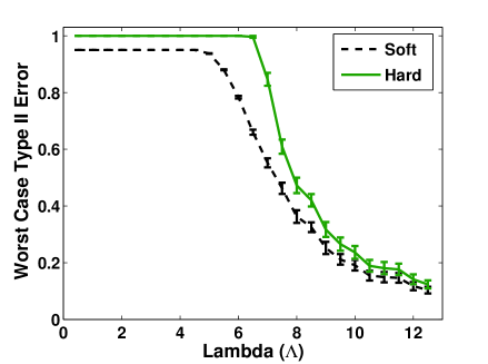
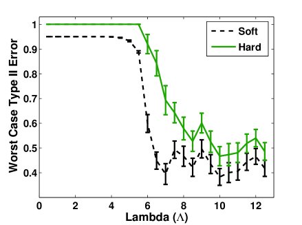
(a) Arbitrary (b) Gaussians

Figure 1: Type II error vs. $\Lambda$, for $N=50$ and $\delta=0.05$. 50 distributions were generated for each value of $\Lambda$ ($\Lambda=0.5,0.1,\cdots,12.5$). Error bars depict standard error of the mean (SEM).

6.2.1 Numerical Examples

We numerically compare the performance of hard and soft rejection strategies for a constrained game, where $D(Q||P)\geq\Lambda$, for various values of $\Lambda$, and two different families of target distributions, $P$, over a support of size $N=50$. The families are arbitrary probability mass functions over $N$ events and discretized Gaussians (over $N$ bins). For each $\Lambda$ we generated 50 random distributions $P$ for each of the families. For each such $P$ we solved the optimal hard and soft strategies and computed the corresponding worst-case optimal type II error, $1-\rho(r,Q)$.

Since $\max_{Q}D(Q||P)=\log(1/\min_{i}p_{i})$, it is necessary that $\min_{i}p_{i}\leq 2^{-\Lambda}$ when generating $P$ (to ensure that a $\Lambda$-distant $Q$ exists). Distributions in the first family of arbitrarily random distributions, Figure 6.1(a),are generated by sampling a point ($p_{1}$) uniformly in $(0,2^{-\Lambda}]$. The other $N-1$ points are drawn i.i.d. $\sim U(0,1]$, and then normalized so that their sum is $1-p_{1}$. The second family, Figure 6.1(b),are Gaussians centered at $0$ and discretized over $N$ evenly spaced bins in the range $[-10,10]$. A (discretized) random Gaussian $N(0,\sigma)$ is selected by choosing $\sigma$ uniformly in some range $[\sigma_{min},\sigma_{max}]$. $\sigma_{min}$ is set to the minimum $\sigma$ ensuring that the first/last bin will not have “zero” probability (due to limited precision). $\sigma_{max}$ was set so that the cumulative probability in the first/last bin will be $2^{-\Lambda}$, if possible (otherwise $\sigma_{max}$ is arbitrarily set to $10*\sigma_{min}$).

The results for $\delta=0.05$ are shown in Figure 6.1.Other results (not presented) for a wide variety of the problem parameters (e.g., $N$, $\delta$) are qualitatively the same. It is evident that both the soft and hard strategies are ineffective for small $\Lambda$. Clearly, the soft method has significantly lower error than that of the hard (until $\Lambda$ becomes “sufficiently large”).

7 Low Density Rejection in a Continuous Setting

In Section 5 we presented a number of results on LDRS optimality in a simplified finite and discrete setting. In this section, we reconsider LDRS (now only in the hard setting) in a much more general framework where the learner and adversary distributions are infinitely continuous. After defining this general setting we extend theorem 10 of Section 5 on hard LDRS optimality. The resulting Theorem 30 is obtained by assuming that the adversary strategy space is sufficiently large, now satisfying a continuous extension of Property A called Property A${}_{\textrm{cont}}$ (Property C is not required in the continuous setting).

The main contribution of this section is a reduction of the SCC problem to two-class classification problem. The two-class classification is facilitated by sampling points from a synthetically generated “other class.” This other class is generated so that it is uniform over its support, which is appropriately selected around the observed support of $P$. Using this synthetic sample we obtain a binary training set on which we can train a soft binary classifier. The final $\delta$-valid SCC classifier is then identified by selecting a threshold on the classifier output so as to maximize the type I error up to $\delta$. The entire routine is simple, practical and if the underlying two-class soft classifier learning algorithm runs in $C(n)$ time complexity, our SCC algorithm runs in time $O(C(n)+n)$. An alternative approach where a hard two-class classifier can be used is described by Nisenson2010.

We show that the SCC routine obtained using this approach is consistent in the sense that if the underlying classification device is consistent then the resulting one-class classifier is asymptotically an LDRF, thus providing an optimal SCC solution when the adversary strategy space satisfies Property A${}_{\textrm{cont}}$.

7.1 Definitions

The SCC problem in the continuous setting is essentially the same as in the finite case (see Section 2) but now both the source distribution $P$ and the adversary distribution can be infinitely continuous distributions over ${\mathbb{R}}^{d}$. Let $\lambda$ be the Lebesgue measure on ${\mathbb{R}}^{d}$. We assume that $P$ is absolutely continuous with respect to $\lambda$ (in other words, if a Borel set $b$ has zero volume in ${\mathbb{R}}^{d}$, then $P(b)=0$). Denote by $p$ the density function of $P$ and let $\mathop{\mathrm{supp}}(p)$ be its support in ${\mathbb{R}}^{d}$.

We define the function ${\mathbb{I}}_{b}(x){\stackrel{{\scriptstyle\vartriangle}}{{=}}}{\mathbb{I}}(x\in b)$, where ${\mathbb{I}}(\cdot)$ is the indicator function. For a Borel set $b$, we define $l_{p}(b){\stackrel{{\scriptstyle\vartriangle}}{{=}}}b\bigcup\{x:p(x)=0\}$.

Definition 26 (Minimum Volume Set).

A set $b\subseteq\mathop{\mathrm{supp}}(p)$ is called a minimum volume set of measure $1-\delta$ if $P(b)=1-\delta$ and for all $b^{\prime}$ such that $P(b^{\prime})=P(b)=1-\delta$, $\lambda(b)\leq\lambda(b^{\prime})$.

Definition 27 (Low Density Set).

1. Let $b\subseteq\mathop{\mathrm{supp}}(p)$ be a minimum volume set of measure $1-\delta$. Let $m$ be any set such that $P(m)=\delta$ and $b\bigcap m=\emptyset$. Then, we call $m$ a core low density set w.r.t. $P$ and $\delta$,

2. Denote by ${\textrm{core}_{\delta}(P)}$ the set of all core low-density sets w.r.t. $P$ and $\delta$.

3. We call a set $s$ a low density set w.r.t. $P$ and $\delta$ if there exists an $m\in{\textrm{core}_{\delta}(P)}$ such that $s=l_{p}(m)$.

7.2 LDRS optimality in the continuous setting

Definition 28 (Low-Density Rejection Strategy (LDRS) and Function (LDRF)).

We define

$$LDRS_{\delta}(P){\stackrel{{\scriptstyle\vartriangle}}{{=}}} \left\{r(\cdot):\;\exists m\in{\textrm{core}_{\delta}(P)}\;s.t.\;r(\cdot)\equiv{\mathbb{I}}_{l_{P}(m)}(\cdot)\right\}.$$

Any function $r(\cdot)\in LDRS_{\delta}(P)$ is called a $\delta$-tight Low-Density Rejection Function (LDRF), and the Low-Density Rejection Strategy is to choose any $\delta$-tight LDRF.

Definition 29 (Property A${}_{\textrm{cont}}$).

We say that two Borel sets $j,k$ satisfy condition $(*)$ if: (i) $j,k\subset\mathop{\mathrm{supp}}(p)$; (ii) $j\cap k=\emptyset$; (iii) $P(j)=P(k)$; and (iv) $\lambda(j)\geq\lambda(k)$.

An adversary strategy space ${\mathcal{Q}}$ has Property A${}_{\textrm{cont}}$ w.r.t $P$, if for every pair $j,k$ satisfying $(*)$: $\forall Q\in{\mathcal{Q}}$ such that $Q(j)<Q(k)$, $\exists Q^{\prime}\in{\mathcal{Q}}$, for which

1. $Q^{\prime}(j)+Q(j)\geq Q^{\prime}(k)+Q(k)$;

2. For all Borel sets $b$ for which $b\bigcap\left(j\bigcup k\right)=\emptyset$, $Q^{\prime}(b)=Q(b)$.

The proof of the following theorem can be found in the appendix.

Theorem 30.

When the learner is restricted to hard-decisions and ${\mathcal{Q}}$ satisfies Property A${}_{\textrm{cont}}$ w.r.t. $P$, then LDRS is optimal.

7.3 SCC via Two-Class Classification

We propose an SCC routine that relies on a soft binary classifier induction. We can use any two-class algorithm, which is consistent in the sense that it minimizes a loss function $\phi(\cdot)$ that is non-negative, differentiable, convex, strictly convex over $[-\infty,0)$ and satisfies $\phi^{\prime}(0)<0$. These conditions are similar but stronger than the conditions required by Bartelett_loss, which provide necessary and sufficient conditions for a convex $\phi$ to be classification-calibrated. We note however that the commonly used loss functions as discussed in Bartelett_loss satisfy our conditions, including the quadratic, truncated-quadratic, exponential and logistic loss functions, to name a few. In the extensions to this section <see¿Nisenson2010 an SCC routine is presented that can utilize any hard binary classifier induction algorithm that minimizes either the 0/1, $L_{1}$, or hinge loss functions, as well as any of the loss functions defined by Bartelett_loss.

Our SCC algorithm is given a training sample $S_{n}=\{x_{1},\ldots,x_{n}\}$ of $n$ training examples drawn i.i.d. from an unknown source distribution $P$ over ${\mathbb{R}}^{d}$. Given a type-I threshold $\delta$ the algorithm outputs a hard rejection function $r(\cdot)$ over ${\mathbb{R}}^{d}$. The main idea of the algorithm is based on the following observation. If our domain is bounded, we can define a two-class classification problem where the first class is $P$ and the other class is a uniform distribution over the (bounded) domain. Then, the output of a consistent soft binary classifier is strictly monotonically increasing with $p(\cdot)$ (the density of $P$) over the support of $P$ (it is only weakly monotone in $p(\cdot)$ over the whole domain). Therefore, thresholding the classifier’s output, with an appropriate quantile, identifies a $\delta$-valid level-set in $P$, inducing a rejection function.

In practice, sampling from a uniform distribution over large domains is computationally hard and moreover, undefined for unbounded domains. Our algorithm avoids these obstacles by sampling uniformly in grid cells containing sampled points from $P$. An additional complication arises in cases where the density $p$ is flat over some regions, which results in discontinuities of the level sets. This is a known issue in level set estimation and is often avoided by assuming that there are no flat regions in $p$, in particular in regions corresponding to the $\delta$ level set Tsybakov (1997); Molchanov (1990). We don’t assume this; our algorithm handles flat regions in $p$ by jittering the classifier output using a small and vanishing (in $n$) random noise (see step 6 in the algorithm below). The resulting algorithm is computationally efficient and practical.

A major component of our algorithm is determining a threshold by quantile estimation. This occurs in Step 7 of the algorithm. We apply a known estimator Uhlmann (1963); Zieliński (2004) that is unbiased and has certain optimal characteristics (see below). This quantile estimator assumes that the cumulative distribution function (cdf), $F$, underlying the sample, is continuous, and is defined over ${\mathbb{R}}$ (i.e., $F$ is the cdf of a real random variable). Let $t_{\mu}$ be the estimate of the $\mu$-quantile of $F$, given $n$ sample points drawn i.i.d. according to $F$. The estimator is unbiased if ${\mathbf{E}}_{F}[F(t_{\mu})]=\mu$. Its variance is $Var_{F}[F(t_{\mu})]$. The estimator we use is called the “uniformly minimum variance unbiased estimator.” It was introduced by Uhlmann63 and we rely on analysis by Zielinski04. This estimator can only be used for estimating $\mu$-quantiles that satisfy $\frac{1}{n+1}\leq\mu\leq\frac{n}{n+1}$, which is equivalent to requiring that $n\geq\max\left\{\frac{\mu}{1-\mu},\frac{1-\mu}{\mu}\right\}$. The estimator chooses an index $\pi_{\mu}$ in $[1,\dots,n]$, and the estimate of the $\mu$-quantile is the $\pi_{\mu}$-th order statistic; in other words, if our sample points are sorted in increasing order, then the estimate is the $\pi_{\mu}$-th element. $\pi_{\mu}$ is calculated as follows:

• Set $k{\stackrel{{\scriptstyle\vartriangle}}{{=}}}\lfloor(n+1)\mu\rfloor$.

• Set $\beta{\stackrel{{\scriptstyle\vartriangle}}{{=}}}(n+1)\mu-k$.

• With probability $\beta$, set $\pi_{\mu}=k+1$, and with probability $1-\beta$, set $\pi_{\mu}=k$.

The estimator’s variance is Zieliński (2004):

$$\frac{\beta(1-\beta)}{(n+1)(n+2)}+\frac{\mu(1-\mu)}{n+2}.$$

The variance is maximized when $\beta=\mu=\frac{1}{2}$, and thus the variance is at most $\frac{1}{4(n+1)}$. Moreover, according to Zielinski04, the estimator is unbiased and its variance is not greater than that of any other unbiased estimator within the family of estimators that can be defined using a probability distribution over single order statistics. For very small samples with $n<\max\left\{\frac{\mu}{1-\mu},\frac{1-\mu}{\mu}\right\}$, we “fall-back” to a simple “default” estimator, which sets $\pi_{\mu}{\stackrel{{\scriptstyle\vartriangle}}{{=}}}\lceil n\mu\rceil$. We term this quantile-estimation algorithm the “uniformly minimum variance unbiased (with fall-back) estimator,” or the “UMVUFB estimator.”

The algorithm is as follows:

1. Define a grid over ${\mathbb{R}}^{d}$ with arbitrary origin and positive cell side length $g_{n}$. Let $g_{n}\to 0$, be such that $ng^{d}\to\infty$. For example, $g_{n}{\stackrel{{\scriptstyle\vartriangle}}{{=}}}n^{-\frac{1}{d+2}}$. Select an arbitrary origin $x_{0}$, for example, uniformly at random from the unit-hypercube. For any point $x=(x^{(1)},\ldots,x^{(d)})$, define the function

   $$A_{n}(x){\stackrel{{\scriptstyle\vartriangle}}{{=}}}\left\lfloor\frac{x-x_{0}}{g_{n}}\right\rfloor{\stackrel{{\scriptstyle\vartriangle}}{{=}}}\left(\left\lfloor\frac{x^{(1)}-x_{0}^{(1)}}{g_{n}}\right\rfloor,\left\lfloor\frac{x^{(2)}-x_{0}^{(2)}}{g_{n}}\right\rfloor,\dots,\left\lfloor\frac{x^{(d)}-x_{0}^{(d)}}{g_{n}}\right\rfloor\right).$$

   For each point $x$, $A_{n}(x)$ specifies the coordinates of the “lower left” corner of the grid cell containing $x$.

2. Define the set $G^{n}_{P}=\bigcup_{x\in S_{n}}A_{n}(x)$ of covered grid cell corners.

3. Generate an artificial sample $O_{n}$ of size $n$ from the “other class.” Each point is selected independently at random as follows:

   1. Choose $a\in G^{n}_{P}$ uniformly at random.

   2. Choose a point $x$ uniformly at random from the unit-hypercube.

   3. The new artificial sample point is $o{\stackrel{{\scriptstyle\vartriangle}}{{=}}}a+g_{n}\cdot x$.

4. Using the training sample consisting of $S_{n}$ (labeled $+1$) and $O_{n}$ (labeled $-1$), train a soft binary classifier $h_{n}(\cdot)$.

5. Define a confidence margin for the $\delta$ threshold. Select any $\theta_{n}\to\infty$ such that $\theta_{n}=o(\sqrt{n})$, for example, take $\theta_{n}{\stackrel{{\scriptstyle\vartriangle}}{{=}}}\sqrt[3]{n}$. Now define $\delta^{+}_{n}{\stackrel{{\scriptstyle\vartriangle}}{{=}}}\delta+\frac{1}{\theta_{n}}$. Choose $\delta^{-}_{n}\leq\delta-\frac{1}{\theta_{n}}$ be such that $\delta^{-}_{n}\to\delta$.

6. Jitter the classifier output. Let $X_{P}$ be a random variable where $X_{P}\sim P$ and $Y_{n}{\stackrel{{\scriptstyle\vartriangle}}{{=}}}h_{n}(X_{p})$. Let $\Phi(\cdot)$ be the cumulative distribution function of $N(0,1)$, and let $m_{n}$ be such that $\frac{\Phi(-m_{n})}{\Phi(m_{n})}=o\left(\frac{1}{\theta_{n}}\right)$, for example $m_{n}{\stackrel{{\scriptstyle\vartriangle}}{{=}}}e^{n}$. Let $\sigma_{n}{\stackrel{{\scriptstyle\vartriangle}}{{=}}}o\left(\frac{1}{m_{n}}\right)$, for example, $\sigma_{n}{\stackrel{{\scriptstyle\vartriangle}}{{=}}}\frac{e^{-n}}{m_{n}}=e^{-2n}$. Let $\varepsilon\sim N[0,\sigma^{2}_{n}]$, and set $Z_{n}{\stackrel{{\scriptstyle\vartriangle}}{{=}}}Y_{n}+\varepsilon$.

7. We use the following threshold mechanism. We will select two thresholds $t^{-}_{n}$ and $t^{+}_{n}$ on $Z_{n}$. The cutoff is always $t^{-}_{n}$ and it is inclusive when $t^{-}_{n}<t^{+}_{n}$. Specifically, let $t^{-}_{n}$ and $t^{+}_{n}$ be estimates of the $\left(\Phi(m_{n})\delta^{-}_{n}+\frac{\Phi(-m_{n})}{2}\right)$-quantile and $\left(\Phi(m_{n})\delta^{+}_{n}+\frac{\Phi(-m_{n})}{2}\right)$-quantile of $Z_{n}$, respectively. In order to establish these estimates we require a sample from $Z_{n}$. The following procedure produces a list of sample points $S_{Z}$.

   • Set $S_{Z}=[]$, i.e. $S_{Z}$ is an empty list.

   • For each $x\in S_{n}$: Choose a value $\epsilon_{x}\sim N[0,\sigma_{n}^{2}]$ and append the value $h_{n}(x)+\epsilon_{x}$ onto $S_{Z}$.

   The sample $S_{z}$ is then the input to the UMVUFB estimator defined above.

8. Define the rejection function

   $$r_{n}(x){\stackrel{{\scriptstyle\vartriangle}}{{=}}}\begin{cases}1&A_{n}(x)\not\in G^{n}_{P};\\ {\mathbb{I}}(h_{n}(x)\leq t^{-}_{n})&A_{n}(x)\in G^{n}_{P}\textrm{ and }\;t^{-}_{n}<t^{+}_{n};\\ {\mathbb{I}}(h_{n}(x)<t^{-}_{n})&\textrm{ otherwise. }\end{cases}$$

Remark 31.

Instead of a soft classifier, $h_{n}(\cdot)$ could have been any consistent class-probability estimator, where $h_{n}(x)$ is the estimate of $\Pr\{+1|x\}$. See Nisenson (2010) for details. $h_{n}(\cdot)$ could also be a consistent ranking algorithm <see, e.g.,¿ClemenconLugosiaVayatis05. In this case, the quantile estimator must select a single sample point to represent the quantile. All comparison operations (e.g. $<$, $\leq$), including those done by the quantile estimator, must be performed by the ranking algorithm. The ranking algorithm must also be able to distinguish between $t^{-}_{n}<t^{+}_{n}$ and $t^{-}_{n}=t^{+}_{n}$.

Let $U_{n}$ (with density $u_{n}$) be the distribution of $O_{n}$ (defined in Step 3). Clearly, $u_{n}$ is uniform over its bounded support. As previously noted, if the support of the generated distribution is significantly larger than that of $P$, an exorbitant number of points may need to be generated in practice in order to reject low density areas in $P$ Davenport . (2006). The following lemma shows that the probability of generating points outside of $p$’s support, almost surely tends to zero.

Lemma 32.

$U_{n}({\mathbb{R}}^{d}\setminus\mathop{\mathrm{supp}}(p))\stackrel{{\scriptstyle\mathrm{a.s.}}}{{\longrightarrow}}0$.

Proof  Recall that $g_{n}$ is a sequence of positive numbers such that $\lim_{n\to\infty}ng_{n}^{d}=\infty$ and $\lim_{n\to\infty}g_{n}=0$. Define a sequence of positive numbers $g^{\prime}_{n}$, such that $g^{\prime}_{n}\geq 2g_{n}$, $g^{\prime}_{n}\to 0$ and $\lim_{n\to\infty}\frac{n{g^{\prime}}_{n}^{d}}{\log n}=\infty$. Define $A(x,g^{\prime}_{n}){\stackrel{{\scriptstyle\vartriangle}}{{=}}}\{y:y\in{\mathbb{R}}^{d}\textrm{ and }||x-y||_{\infty}\leq g^{\prime}_{n}\}$. Define $T_{n}{\stackrel{{\scriptstyle\vartriangle}}{{=}}}\bigcup_{i=1}^{n}A(x_{i},g^{\prime}_{n})$. DevroyeWise80 show that for any probability measure $\nu$ on the Borel sets of ${\mathbb{R}}^{d}$ whose restriction to $\mathop{\mathrm{supp}}(p)$ is absolutely continuous w.r.t. $P$, it holds that $\nu(T_{n}\mathop{\Delta}\mathop{\mathrm{supp}}(p))\stackrel{{\scriptstyle\mathrm{a.s.}}}{{\longrightarrow}}0$. We note that the grid cell of $x$ is always a sub-region of $A(x,g^{\prime}_{n})$, and therefore $\mathop{\mathrm{supp}}(u_{n})\subseteq T_{n}$. Thus, noting that $U_{n}({\mathbb{R}}^{d}\setminus\mathop{\mathrm{supp}}(p))=U_{n}(\mathop{\mathrm{supp}}(u_{n})\setminus\mathop{\mathrm{supp}}(p))$,

$$U_{n}(\mathop{\mathrm{supp}}(u_{n})\setminus\mathop{\mathrm{supp}}(p)) \leq\sup_{m}U_{m}(\mathop{\mathrm{supp}}(u_{n})\setminus\mathop{\mathrm{supp}}(p))$$

$$\leq\sup_{m}U_{m}(T_{n}\setminus\mathop{\mathrm{supp}}(p))$$

$$\leq\sup_{m}U_{m}(T_{n}\mathop{\Delta}\mathop{\mathrm{supp}}(p))$$

$$\Rightarrow\lim_{n\rightarrow\infty}U_{n}(\mathop{\mathrm{supp}}(u_{n})\setminus\mathop{\mathrm{supp}}(p)) \leq\lim_{n\rightarrow\infty}\sup_{m}U_{m}(T_{n}\mathop{\Delta}\mathop{\mathrm{supp}}(p))$$

$$=\sup_{m}\lim_{n\to\infty}U_{m}(T_{n}\mathop{\Delta}\mathop{\mathrm{supp}}(p))$$

$$\stackrel{{\scriptstyle\mathrm{a.s.}}}{{=}}0.$$

 

Remark 33.

It is difficult to establish exact convergence rates in Lemma 32 without constraints on $P$. For cases where $\lambda({\mathbb{R}}^{d}\setminus\mathop{\mathrm{supp}}(p))=0$, we obviously have that $U_{n}({\mathbb{R}}^{d}\setminus\mathop{\mathrm{supp}}(p))=0$. This is the case, for example, for finite mixtures of Gaussians.

If there exists a constant $K$, such that $|p(x)-p(y)|\leq K$ whenever $||x-y||_{\infty}\leq g_{n}$, we can establish an upper bound on the rate. The condition $||x-y||_{\infty}\leq g_{n}$ is equivalent to $x$ and $y$ being in the same grid-cell. Therefore, if $p(x)>K$, then for all $y$ in the same grid-cell, $p(y)>0$. Note that if $p$ is Lipschitz continuous such that $|p(x)-p(y)|\leq\frac{K}{g_{n}}||x-y||_{\infty}$, then $p$ meets the above condition. Let $1-\eta$ be a desired confidence level. Let $C^{\eta}_{K}$ be the number of cells in the grid which contain more than $Kng_{n}^{d}+\sqrt{\frac{n(\ln|G^{n}_{p}|-\ln\eta)}{2}}$ sample points. Then, using Hoeffding’s inequality, it isn’t hard to show that with probability at least $1-\eta$, $U_{n}({\mathbb{R}}^{d}\setminus\mathop{\mathrm{supp}}(p))\leq 1-\frac{C^{\eta}_{K}}{|G^{n}_{P}|}$.

Definition 34 (Quantile).

Let $\xi$ be a random variable whose domain is in ${\mathbb{R}}$. We say that $t$ is a $\mu$-quantile of $\xi$ if

$$t\in S_{\xi}(\mu){\stackrel{{\scriptstyle\vartriangle}}{{=}}}\left\{\tau\in{\mathbb{R}}:\Pr\{\xi<\tau\}\leq\mu\textrm{ and }\Pr\{\xi\leq\tau\}\geq\mu\right\}.$$

Define a new random variable $\kappa$ to represent the level sets of $P$. Formally, its cumulative distribution function is $F_{\kappa}(t)=P(\{x:p(x)\leq t\})$.

Definition 35.

Let $v$ be any $\delta$-quantile of $\kappa$. We say $P$ has a $\delta$-jump if $F_{\kappa}(v)>\delta$.

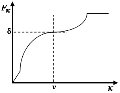
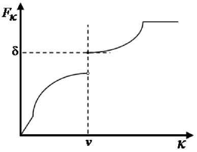
(a) (b)

Figure 2: The cumulative distribution function $F_{\kappa}$ when $P$ doesn’t have a $\delta$-jump.

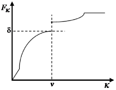
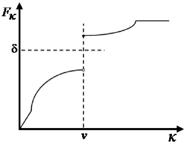
(a) (b)

Figure 3: The cumulative distribution function $F_{\kappa}$ when $P$ does have a $\delta$-jump.

We now will consider two cases, one where $P$ doesn’t have a $\delta$-jump and one where it does. See Figure 2 and Figure 3. In all figures the (unique) $\delta$-quantile of $\kappa$ is marked by $v$. Note that a quantile need not be unique, in particular there will be a range of values wherever $F_{\kappa}$ is flat.

Definition 36.

A rejection function $r(\cdot)$ is called a $\delta$-maximal level-set estimator for $P$ if, for some $v\in S_{\kappa}(\delta)$, either:

1. $P$ doesn’t have a $\delta$-jump and $r(x)\equiv{\mathbb{I}}(p(x)\leq v)$, almost everywhere.

2. $P$ has a $\delta$-jump and $r(x)\equiv{\mathbb{I}}(p(x)<v)$, almost everywhere.

Note that if $P$ doesn’t have a $\delta$-jump, then a $\delta$-maximal level-set estimator for $P$ is a $\delta$-tight LDRF. We will now prove that the output of the algorithm is asymptotically (almost surely) a $\delta$-maximal level-set estimator for $P$.

Theorem 37.

Let $\{U^{\prime}_{n}\}$, $n=1,2,\ldots,$ be a sequence of probability measures such that for each $n$, $U^{\prime}_{n}$ has uniform density $u^{\prime}_{n}$ over its bounded support, and $\lim_{n\to\infty}P(\mathop{\mathrm{supp}}(u^{\prime}_{n}))=1$. Define a Bayesian binary classification problem for each $n$. Let the first class, $c_{1}\equiv+1$ have distribution $P$, and the second class $c_{2}\equiv-1$ have distribution $U^{\prime}_{n}$. The classes’ prior probabilities are $\Pr\{+1\}=\Pr\{-1\}=\frac{1}{2}$. Let $\phi(\cdot)$ be a non-negative, differentiable, convex loss function such that it is strictly convex on $[-\infty,0)$ and $\phi^{\prime}(0)<0$. Let $h^{*}_{n}(\cdot)$ be the soft Bayes-optimal classifier that minimizes the expected loss. Define a random variable $Y^{*}_{n}{\stackrel{{\scriptstyle\vartriangle}}{{=}}}h^{*}_{n}(X_{P})$. Let $t^{*}_{n}$ be a $\delta$-quantile of $Y^{*}_{n}$. Define the rejection function:

$$r^{*}_{n}(x){\stackrel{{\scriptstyle\vartriangle}}{{=}}}\begin{cases}1&x\not\in\mathop{\mathrm{supp}}(u^{\prime}_{n});\\ {\mathbb{I}}(h^{*}_{n}(x)\leq t^{*}_{n})&x\in\mathop{\mathrm{supp}}(u^{\prime}_{n})\textrm{ and $P$ doesn't have a $\delta$-jump};\\ {\mathbb{I}}(h^{*}_{n}(x)<t^{*}_{n})&\textrm{ otherwise. }\end{cases}$$

Then, $r^{*}(\cdot){\stackrel{{\scriptstyle\vartriangle}}{{=}}}\lim_{n\to\infty}r^{*}_{n}(\cdot)$ is a $\delta$-maximal level-set estimator for $P$.

Proof  We first consider $x\in\mathop{\mathrm{supp}}(u^{\prime}_{n})$. Define the function $\psi_{n}(x){\stackrel{{\scriptstyle\vartriangle}}{{=}}}\frac{p(x)}{u^{\prime}_{n}(x)}$, defined over $\mathop{\mathrm{supp}}(u^{\prime}_{n})$. From Bayes theorem, it is not hard to show that $\Pr\{+1|x\}=\frac{p(x)}{p(x)+u^{\prime}_{n}(x)}$. The loss for a point $x$ when we assign it value $y$ is Bartlett . (2006):

$$\ell(x,y){\stackrel{{\scriptstyle\vartriangle}}{{=}}} \Pr\{+1|x\}\phi(y)+\Pr\{-1|x\}\phi(-y)$$

$$=\frac{p(x)\phi(y)+u^{\prime}_{n}(x)\phi(-y)}{p(x)+u^{\prime}_{n}(x)}.$$

It is easy to verify that for a fixed $x$, at the minimum (over $y$) of $\ell(x,y)$, $p(x)\phi^{\prime}(y)=u^{\prime}_{n}(x)\phi^{\prime}(-y)$. Alternatively: $\phi^{\prime}(-y)=\psi_{n}(x)\phi^{\prime}(y)$. Let $x_{1}$ and $x_{2}$ be two points such that $\psi_{n}(x_{1})>\psi_{n}(x_{2})$. Note that $\min\{\phi^{\prime}(y),\phi^{\prime}(-y)\}\leq\phi^{\prime}(0)<0$ for all $y$. Let $c_{i}{\stackrel{{\scriptstyle\vartriangle}}{{=}}}\psi_{n}(x_{i})$ and $y_{i}$ be a solution to $\phi^{\prime}(-y)=c_{i}\phi^{\prime}(y)$, for $i\in\{1,2\}$. Note that $c_{1},c_{2}\geq 0$ and therefore, in order for equality to occur it is necessary that $\phi^{\prime}(y_{i}),\phi^{\prime}(-y_{i})\leq 0$ (with equality only if $c_{i}=0$). We can now rewrite $\phi^{\prime}(-y_{i})=c_{i}\phi^{\prime}(y_{i})$ as $|\phi^{\prime}(-y_{i})|=c_{i}|\phi^{\prime}(y_{i})|$.

We will now prove that $y_{1}>y_{2}$. Assume by contradiction that the statement is false. Then $y_{2}\geq y_{1}$. Therefore, $|\phi^{\prime}(y_{2})|\leq|\phi^{\prime}(y_{1})|$ and $|\phi^{\prime}(-y_{2})|\geq|\phi^{\prime}(-y_{1})|$. Since $\psi_{n}(x_{1})>\psi_{n}(x_{2})$, it follows that $c_{1}>c_{2}$. If $c_{2}=0$, then $0=|\phi^{\prime}(-y_{2})|\geq|\phi^{\prime}(-y_{1})|$. Therefore $\phi^{\prime}(-y_{1})=0$ and $\phi^{\prime}(y_{1})<0$, which gives $0=|\phi^{\prime}(-y_{1})|=c_{1}|\phi^{\prime}(y_{1})|<0$, which is a contradiction. Thus, $c_{2}\neq 0$, and $|\phi^{\prime}(-y_{2})|=c_{2}|\phi^{\prime}(y_{2})|\leq c_{2}|\phi^{\prime}(y_{1})|=\frac{c_{2}}{c_{1}}|\phi^{\prime}(-y_{1})|\leq\frac{c_{2}}{c_{1}}|\phi^{\prime}(-y_{2})|<|\phi^{\prime}(-y_{2})|$. Contradiction.

Now consider the case where $c_{i}=\frac{|\phi^{\prime}(-y_{i})|}{|\phi^{\prime}(y_{i})|}>0$. Therefore, $\phi^{\prime}(y_{i}),\phi^{\prime}(-y_{i})<0$. Since $\phi(\cdot)$ is strictly convex over $[-\infty,0)$ it follows that as $y_{i}$ increases $|\phi^{\prime}(y_{i})|$ decreases and $|\phi^{\prime}(-y_{i})|$ increases. Therefore, if $\psi_{n}(x_{1})=\psi_{n}(x_{2})>0$, there is a unique solution.

Therefore, $h^{*}_{n}(x)$ is monotonically increasing with $\psi_{n}(x)$, almost everywhere over $\mathop{\mathrm{supp}}(u_{n})$ and strictly monotonically increasing with $\psi_{n}(x)$, almost everywhere over $\mathop{\mathrm{supp}}(u_{n})\bigcap\mathop{\mathrm{supp}}(p)$. Since $u^{\prime}_{n}(\cdot)$ is constant over its support, this implies: $p(x_{1})<p(x_{2})\Rightarrow h^{*}_{n}(x_{1})<h^{*}_{n}(x_{2})$, and $0<p(x_{1})=p(x_{2})\Rightarrow h^{*}_{n}(x_{1})=h^{*}_{n}(x_{2})$. Therefore, for some $v^{*}_{n}$, $\{x\in\mathop{\mathrm{supp}}(u^{\prime}_{n})\bigcap\mathop{\mathrm{supp}}(p):h^{*}_{n}(x)\leq t^{*}_{n}\}$ is identical to $\{x\in\mathop{\mathrm{supp}}(u^{\prime}_{n})\bigcap\mathop{\mathrm{supp}}(p):p(x)\leq v^{*}_{n}\}$ (with the possible exception of a set of points of zero Lebesgue measure). Recalling that $Y^{*}_{n}=h^{*}_{n}(X_{P})$ for $X_{P}\sim P$ and that $P(\mathop{\mathrm{supp}}(u^{\prime}_{n}))\to 1$:

$$\lim_{n\to\infty}t^{*}_{n}\in \lim_{n\to\infty}\{\tau\in{\mathbb{R}}:\Pr\{Y^{*}_{n}<\tau\}\leq\delta\textrm{ and }\Pr\{Y^{*}_{n}\leq\tau\}\geq\delta\}$$

$$= \lim_{n\to\infty}\{\tau\in{\mathbb{R}}:P(\{x:h^{*}_{n}(x)<\tau\})\leq\delta\textrm{ and }P(\{x:h^{*}_{n}(x)\leq\tau\})\geq\delta\}$$

$$= \lim_{n\to\infty}\{\tau\in{\mathbb{R}}:P(\{x\in\mathop{\mathrm{supp}}(u^{\prime}_{n})\bigcap\mathop{\mathrm{supp}}(p):h^{*}_{n}(x)<\tau\})\leq\delta\textrm{ and }$$

$$\;\;\;\;\;\;\;\;\;\;\;\;\;\;\;\;\;P(\{x\in\mathop{\mathrm{supp}}(u^{\prime}_{n})\bigcap\mathop{\mathrm{supp}}(p):h^{*}_{n}(x)\leq\tau\})\geq\delta\}$$

$$\Rightarrow\lim_{n\to\infty}v^{*}_{n}\in \lim_{n\to\infty}\{\tau^{\prime}\in{\mathbb{R}}:P(\{x\in\mathop{\mathrm{supp}}(u^{\prime}_{n})\bigcap\mathop{\mathrm{supp}}(p):p(x)<\tau^{\prime}\})\leq\delta\textrm{ and }$$

$$\;\;\;\;\;\;\;\;\;\;\;\;\;\;\;\;\;P(\{x\in\mathop{\mathrm{supp}}(u^{\prime}_{n})\bigcap\mathop{\mathrm{supp}}(p):p(x)\leq\tau^{\prime}\})\geq\delta\}$$

$$= \lim_{n\to\infty}\{\tau^{\prime}\in{\mathbb{R}}:P(\{x:p(x)<\tau\})\leq\delta\textrm{ and }P(\{x:p(x)\leq\tau^{\prime}\})\geq\delta\}$$

$$= \{\tau^{\prime}\in{\mathbb{R}}:P(\{x:p(x)<\tau\})\leq\delta\textrm{ and }P(\{x:p(x)\leq\tau^{\prime}\})\geq\delta\}$$

$$= \{\tau^{\prime}\in{\mathbb{R}}:\Pr\{\kappa<\tau^{\prime}\}\leq\delta\textrm{ and }\Pr\{\kappa\leq\tau^{\prime}\}\geq\delta\}$$

$$= S_{\kappa}(\delta)$$

Therefore, let $v^{\delta}_{p}\in S_{\kappa}(\delta)$ be such that $v^{\delta}_{p}=\lim_{n\to\infty}v^{*}_{n}$. Note that since $\delta>0$, $v^{\delta}_{p}>0$ (otherwise $\delta\leq P(\{x:p(x)\leq v^{\delta}_{p})=0$). Therefore, for sufficiently large $n$, $v^{*}_{n}>0$.

Let us assume that $P$ doesn’t have a $\delta$-jump. Therefore, for almost every $x\in\mathop{\mathrm{supp}}(u^{\prime}_{n})$, ${\mathbb{I}}(h^{*}_{n}(x)\leq t^{*}_{n})={\mathbb{I}}(p(x)\leq v^{*}_{n})$. Then almost everywhere in $\mathop{\mathrm{supp}}(u^{\prime}_{n})$: $r(x)=\lim_{n\to\infty}{\mathbb{I}}(h^{*}_{n}(x)\leq t^{*}_{n})={\mathbb{I}}(p(x)\leq v^{\delta}_{p})$. It is given that $P({\mathbb{R}}^{d}\setminus\mathop{\mathrm{supp}}(u^{\prime}_{n}))\to 0$. Therefore, $\lambda(\{x\not\in\mathop{\mathrm{supp}}(u^{\prime}_{n}):p(x)>v^{\delta}_{p}\})\to 0$. which is equivalent to $\lambda(\{x\not\in\mathop{\mathrm{supp}}(u^{\prime}_{n}):{\mathbb{I}}(p(x)\leq v^{\delta}_{p})\neq r^{*}_{n}(x)\})\to 0$.

If $P$ has a $\delta$-jump, the proof is almost identical, only with minor changes in the strengths of inequalities. For almost every $x\in\mathop{\mathrm{supp}}(u^{\prime}_{n})$: $r(x)=\lim_{n\to\infty}{\mathbb{I}}(h^{*}_{n}(x)<t^{*}_{n})={\mathbb{I}}(p(x)<v^{\delta}_{p})$, and $\lambda(\{x\not\in\mathop{\mathrm{supp}}(u^{\prime}_{n}):{\mathbb{I}}(p(x)<v^{\delta}_{p})\neq r^{*}_{n}(x)\})\to 0$.  

We will now make clear the relation between the algorithm given and Theorem 37. Clearly $\{U_{n}\}$ is a series of distributions each having a uniform density, $u_{n}$, over its bounded support. We will now prove that $P(\mathop{\mathrm{supp}}(u_{n}))\stackrel{{\scriptstyle\mathrm{a.s.}}}{{\longrightarrow}}1$.

Lemma 38.

For any $\epsilon>0$, $\Pr\{P(\mathop{\mathrm{supp}}(u_{n}))\leq 1-\epsilon\}\leq 2e^{-2n\epsilon^{2}-no(1)}$ and $P(\mathop{\mathrm{supp}}(u_{n}))\stackrel{{\scriptstyle\mathrm{a.s.}}}{{\longrightarrow}}1$.

Proof  We define $G(x)$ to be the cell in the grid which contains $x$. Define $c(b){\stackrel{{\scriptstyle\vartriangle}}{{=}}}\left|\{S\bigcap b\}\right|$ to be the count of the number of training samples which fall within set $b$. Then the histogram density estimate is $\tilde{p}_{n}(x){\stackrel{{\scriptstyle\vartriangle}}{{=}}}\frac{c\left(G(x)\right)}{nh^{d}}$. As shown by DevroyeGyorfi02 in Theorem 5.6, $\Pr\left\{\int_{{\mathbb{R}}^{d}}|p(x)-\tilde{p}_{n}(x)|\lambda(dx)>2\epsilon\right\}\leq 2e^{-2n\epsilon^{2}-no(1)}$. However, since $P$ is absolutely continuous w.r.t. $\lambda$, it follows from Scheffé’s theorem (Scheffe47, used as Theorem 5.4 by DevroyeGyorfi02), that for any Borel set $B$ over ${\mathbb{R}}^{d}$, $\Pr\left\{\int_{B}|p(x)-\tilde{p}_{n}(x)|\lambda(dx)>\epsilon\right\}\leq 2e^{-2n\epsilon^{2}-no(1)}$.

By definition, $\tilde{p}_{n}(x)=0$ for all $x\not\in\mathop{\mathrm{supp}}(u_{n})$. Therefore:

$$\Pr\left\{P\left({\mathbb{R}}^{d}\setminus\mathop{\mathrm{supp}}(u_{n})\right)>\epsilon\right\}= \Pr\left\{\int_{{\mathbb{R}}^{d}\setminus\mathop{\mathrm{supp}}(u_{n})}|p(x)-\tilde{p}_{n}(x)|\lambda(dx)>\epsilon\right\}$$

$$\leq 2e^{-2n\epsilon^{2}-no(1)}.$$

Since this is true for any $\epsilon$, it immediately follows that $\Pr\{\lim_{n\to\infty}P({\mathbb{R}}^{d}\setminus\mathop{\mathrm{supp}}(u_{n}))\neq 0\}=0$, or $P(\mathop{\mathrm{supp}}(u_{n}))\stackrel{{\scriptstyle\mathrm{a.s.}}}{{\longrightarrow}}1$.  

Therefore, the only remaining part is to show how $t^{-}_{n}$ and $t^{+}_{n}$ relate to $t^{*}_{n}$ and to whether $P$ has a $\delta$-jump or not. We note that for all $x$, at the limit, $h^{*}_{n}(x)=h_{n}(x)$ and therefore, $Y^{*}_{n}\equiv Y_{n}$ (i.e. they are distributed identically). For sufficiently large $n$, the quantile estimator used is unbiased with standard deviation vanishing at a rate of $O\left(\frac{1}{\sqrt{n+1}}\right)$ Zieliński (2004). Therefore, since $\theta_{n}=o(\sqrt{n})$, it follows that $\frac{1}{\sqrt{n}}=o(\frac{1}{\theta_{n}})$, and thus for sufficiently large $n$, $t^{-}_{n}$ and $t^{+}_{n}$ are tightly concentrated around a $\left(\Phi(m_{n})\delta^{-}_{n}+\frac{\Phi(-m_{n})}{2}\right)$-quantile (which is not greater than the $\left(\Phi(m_{n})\left[\delta-\frac{1}{\theta_{n}}\right]+\frac{\Phi(-m_{n})}{2}\right)$-quantile) and a $\left(\Phi(m_{n})\left[\delta+\frac{1}{\theta_{n}}\right]+\frac{\Phi(-m_{n})}{2}\right)$-quantile for $Z_{n}$, respectively. Therefore, since $\frac{\Phi(-m_{n})}{\Phi(m_{n})}=o\left(\frac{1}{\theta_{n}}\right)$, by the following lemma, $t^{-}_{n}$ and $t^{+}_{n}$ are also tightly concentrated around a $\delta^{-}_{n}$-quantile and a $\delta^{+}_{n}$-quantile for $Y_{n}$, respectively.

Lemma 39.

Let $m\geq 0$. Let $t_{\mu}$ be a $\left(\Phi(m)\mu+\frac{\Phi(-m)}{2}\right)$-quantile of $Z_{n}$. Then, for some $\mu^{\prime}$ such that $|\mu^{\prime}-\mu|\leq\frac{\Phi(-m)}{2\Phi(m)}$, a $\mu^{\prime}$-quantile of $Y_{n}$, $t^{*}_{\mu^{\prime}}$, satisfies $|t^{*}_{\mu^{\prime}}-t_{\mu}|\leq m\sigma_{n}$.

Proof 

$$\mu+\frac{\Phi(-m)}{2\Phi(m)}\geq \frac{1}{\Phi(m)}\Pr\{Z_{n}<t\}=\frac{1}{\Phi(m)}\Pr\{Y_{n}<t+\varepsilon\}$$

$$\geq \frac{1}{\Phi(m)}\Pr\{Y_{n}<t-m\sigma_{n}\}\Pr\{\varepsilon\geq-m\sigma_{n}\}=\Pr\{Y_{n}<t-m\sigma_{n}\}$$

$$\mu+\frac{\Phi(-m)}{2\Phi(m)}\leq \frac{1}{\Phi(m)}\Pr\{Z_{n}\leq t\}=\frac{1}{\Phi(m)}\Pr\{Y_{n}\leq t+\varepsilon\}$$

$$\leq \frac{1}{\Phi(m)}\left[\Pr\{Y_{n}\leq t+m\sigma_{n}\}\Pr\{\varepsilon\leq m\sigma_{n}\}+\Pr\{\varepsilon>m\sigma_{n}\}\right]$$

$$\leq \frac{1}{\Phi(m)}\left[\Pr\{Y_{n}\leq t+m\sigma_{n}\}\Phi(m)+\Phi(-m)\right]$$

$$= \Pr\{Y_{n}\leq t+m\sigma_{n}\}+\frac{\Phi(-m)}{\Phi(m)}.$$

Therefore, $\mu+\frac{\Phi(-m)}{2\Phi(m)}\geq\Pr\{Y_{n}<t-m\sigma_{n}\}$ and $\mu-\frac{\Phi(-m)}{2\Phi(m)}\leq\Pr\{Y_{n}\leq t+m\sigma_{n}\}$. Let $\Delta_{1}{\stackrel{{\scriptstyle\vartriangle}}{{=}}}\Pr\{Y_{n}<t-m\sigma_{n}\}-\mu$, and let $\Delta_{2}{\stackrel{{\scriptstyle\vartriangle}}{{=}}}\Pr\{Y_{n}\leq t+m\sigma_{n}\}-\mu$. Note that $t-m\sigma_{n}$ is a $(\mu+\Delta_{1})$-quantile and that $t+m\sigma_{n}$ is a $(\mu+\Delta_{2})$-quantile of $Y_{n}$. Therefore, since $\Delta_{2}\geq\Delta_{1}$, for every $\Delta\in[\Delta_{1},\Delta_{2}]$, there is some $t^{\prime}$ such that $|t^{\prime}-t_{\mu}|\leq m\sigma_{n}$, which is a $(\mu+\Delta)$-quantile of $Y_{n}$. To complete the proof, note that $\Delta_{1}\leq\frac{\Phi(-m)}{2\Phi(m)}$ and $\Delta_{2}\geq-\frac{\Phi(-m)}{2\Phi(m)}$. Therefore, there exists some $\Delta\in\left[-\frac{\Phi(-m)}{2\Phi(m)},\frac{\Phi(-m)}{2\Phi(m)}\right]$ such that $\Delta\in[\Delta_{1},\Delta_{2}]$.  

Theorem 40.

The rejection function output by the algorithm is (almost surely) identical to that of Theorem 37 at the limit, where $U^{\prime}_{n}{\stackrel{{\scriptstyle\vartriangle}}{{=}}}U_{n}$.

Proof  By definition, $x\in\mathop{\mathrm{supp}}(u^{\prime}_{n})\Leftrightarrow A_{n}(x)\in G^{n}_{p}$.

We represent by $t^{*-}_{n}$ and $t^{*+}_{n}$ the $\delta^{-}_{n}$ and $\delta^{+}_{n}$ quantiles of $Y^{*}_{n}$, around which (for sufficiently large $n$), $t^{-}_{n}$ and $t^{+}_{n}$ are tightly concentrated. In particular, $t^{*-}_{n}<t^{*+}_{n}\Rightarrow t^{-}_{n}<t^{+}_{n}$. Note that $t^{-}_{n}\leq t^{+}_{n}$ and $t^{*-}_{n}\leq t^{*}_{n}\leq t^{*+}_{n}$ always, and at the limit, $t^{-}_{n}=t^{*-}_{n}=t^{*}_{n}=t^{*+}_{n}=t^{+}_{n}$. We now consider four cases.

In the first, $P$ doesn’t have a $\delta^{-}_{n}$-jump or a $\delta$-jump (see Figure 7.1(a)).Then, $t^{*-}_{n}<t^{*}_{n}<t^{*+}_{n}$. Therefore, for $x\in\mathop{\mathrm{supp}}(u^{\prime}_{n})$, at the limit: ${\mathbb{I}}(h_{n}(x)\leq t^{-}_{n})={\mathbb{I}}(h^{*}_{n}(x)\leq t^{*}_{n}(x))$.

In the second, $P$ has a $\delta^{-}_{n}$-jump but it doesn’t have a $\delta$-jump (see Figure 7.1(b)).Then, for sufficiently large $n$, $t^{*-}_{n}=t^{*}_{n}<t^{*+}_{n}$ and $\delta^{-}_{n}<\Pr\{Y^{*}_{n}\leq t^{*-}_{n}\}\leq\delta$. Therefore, for $x\in\mathop{\mathrm{supp}}(u^{\prime}_{n})$, at the limit: ${\mathbb{I}}(h_{n}(x)\leq t^{-}_{n})={\mathbb{I}}(h^{*}_{n}(x)\leq t^{*}_{n}(x))$.

In the third, $P$ doesn’t have a $\delta^{-}_{n}$-jump but it does have a $\delta$-jump (see Figure 7.2(a)).Then, for sufficiently large $n$, $t^{*-}_{n}<t^{*}_{n}=t^{*+}_{n}$. Therefore, for $x\in\mathop{\mathrm{supp}}(u^{\prime}_{n})$, at the limit: ${\mathbb{I}}(h_{n}(x)\leq t^{-}_{n})={\mathbb{I}}(h^{*}_{n}(x)<t^{*}_{n}(x))$.

In the fourth, $P$ has both a $\delta^{-}_{n}$-jump and a $\delta$-jump (see Figure 7.2(b)).Then, for sufficiently large $n$, $t^{*-}_{n}=t^{*}_{n}=t^{*+}_{n}$. Therefore, for $x\in\mathop{\mathrm{supp}}(u^{\prime}_{n})$, at the limit: ${\mathbb{I}}(h_{n}(x)<t^{-}_{n})={\mathbb{I}}(h^{*}_{n}(x)<t^{*}_{n}(x))$.  

Remark 41 (Rates of Convergence and Finite Sample Notes).

The time complexity for our algorithm is $O(C(n)+n)$, where $C(n)$ is the time complexity for the soft-classification algorithm. The rate of convergence for the given algorithm is $\Theta\left(\frac{1}{\theta_{n}}\right)=\Theta\left(\frac{1}{n^{\frac{1}{2}+\epsilon}}\right)$, for any $\epsilon>0$, in addition to the classifier’s rate of convergence. $\theta_{n}$ is only affected by the quantile-estimator used. In our case, the quantile estimator utilized only requires that $F$, the cdf whose quantile is being estimated, be continuous. To meet this condition we added the noise term $\varepsilon$. Note that $\varepsilon$ has no effect on the convergence rate; this is because $\sigma_{n}$ can vanish as fast as desired. Similarly, by Lemma 39, we can achieve arbitrarily tight bounds on the nearness of the quantiles of $Z_{n}$ and $Y_{n}$ by increasing the rate at which $m_{n}$ tends to infinity.

For finite sample sizes, some additional modifications are advisable. First, in order to ensure that $h^{*}_{n}(\cdot)={\mathbf{E}}_{U_{n}}[h_{n}(\cdot)]$, $O_{n}$ should be of size $n^{\prime}\sim NB(n,\frac{1}{2})$, and not $n$. It is also possible to use a non-uniform prior probability (without affecting the algorithm’s correctness), if it is desired. A validation set could be used for determining the quantile-estimates, rather than the training set. Note that for finite samples, it is not guaranteed that $\Pr\{Y_{n}\leq t^{-}_{n}\}\approx\delta^{-}_{n}$. In fact, it is possible to be significantly larger if $Y_{n}$ has a large jump in the range $[t^{-}_{n}-m\sigma_{n},t^{-}_{n})$. Since by Lemma 39, $\Pr\{Y_{n}\leq t^{-}_{n}-m\sigma_{n}\}\leq\delta^{-}_{n}+\frac{\Phi(-m)}{2\Phi(m)}+o\left(\frac{1}{\theta_{n}}\right)$, almost surely, we can address this issue by refining the definition of the rejection function output by the algorithm:

$$r_{n}(x){\stackrel{{\scriptstyle\vartriangle}}{{=}}}\begin{cases}1&A_{n}(x)\not\in G^{n}_{P};\\ {\mathbb{I}}(h_{n}(x)\leq t^{-}_{n}-m\sigma_{n})&A_{n}(x)\in G^{n}_{P}\textrm{ and }\;t^{-}_{n}<t^{+}_{n};\\ {\mathbb{I}}(h_{n}(x)<t^{-}_{n}-m\sigma_{n})&\textrm{ otherwise. }\end{cases}$$

Note that this fix isn’t possible when using a ranking algorithm in place of a soft binary classifier, since only points, and not values, can be compared (i.e., $x$ and the chosen quantile point in $S_{Z}$ are compared in order to determine whether to reject $x$).

Finally, one needs to determine $\delta^{-}_{n}$, so that it is guaranteed (with high probability) that $\rho(r_{n},P)\leq\delta$. To accomplish this, one must take into account the quantile estimator used, since $\delta^{-}_{n}\leq\delta-\frac{1}{\theta_{n}}$, and $P({\mathbb{R}}^{d}\setminus\mathop{\mathrm{supp}}(u_{n}))$, since this is always rejected. It is known Hall  Hannan (1988) for the histogram density estimator, upon which the sampling of $O_{n}$ in the algorithm is loosely-based, that $g_{n}$ of order $n^{-\frac{1}{d+2}}$ is optimal for minimizing $L_{b}$ distance for $1\leq b<\infty$, and that $g_{n}$ of order $\left(\frac{\log n}{n}\right)^{\frac{1}{d+2}}$ is the correct order for minimizing $L_{\infty}$ distance. However, we are only interested in $P({\mathbb{R}}^{d}\setminus\mathop{\mathrm{supp}}(u_{n}))$. We note that this is just the missing mass. Let $n_{1}$ be the number of grid cells containing exactly one point from the sample. Then, as shown by McallesterSchapire2000, with probability at least $1-\eta$, $P({\mathbb{R}}^{d}\setminus\mathop{\mathrm{supp}}(u_{n}))\leq\frac{n_{1}}{n}+\left(2\sqrt{2}+\sqrt{3}\right)\sqrt{\frac{\ln{3}-\ln{\eta}}{n}}$. Clearly, increasing $g_{n}$ results in $n_{1}$ decreasing. Therefore, $g_{n}$ should be large in order to minimize $P({\mathbb{R}}^{d}\setminus\mathop{\mathrm{supp}}(u_{n}))$ and small in order to minimize $U_{n}({\mathbb{R}}^{d}\setminus\mathop{\mathrm{supp}}(p))$ (since if $g_{n}$ vanishes faster, $\lambda(\mathop{\mathrm{supp}}(u_{n})\setminus\mathop{\mathrm{supp}}(p))$ decreases faster as well). This results in a simple heuristic, namely to set $g_{n}$ to the smallest value such that $n_{1}\leq t$, for some threshold $t$. For example, if we know the sample is “clean” in the sense that all points are drawn i.i.d. according to $P$, then we can take $t=0$. A larger value of $t$ could be chosen were we to suspect that the sample may contain noise, for example $t=\log{n}$. In general, it remains an open question of how $g_{n}$ should be optimized to balance between $P({\mathbb{R}}^{d}\setminus\mathop{\mathrm{supp}}(u_{n}))$ and $U_{n}({\mathbb{R}}^{d}\setminus\mathop{\mathrm{supp}}(p))$.

Remark 42.

Cuevas97 use a plug-in approach to support estimation that can be leveraged here to further decrease $U_{n}({\mathbb{R}}^{d}\setminus\mathop{\mathrm{supp}}(p))$ when $p$ has compact support and is continuously differentiable. Let $g_{n}=cn^{-\frac{1}{d+2}}$ for some constant $c$, and let $\alpha_{n}$ be such that $\alpha_{n}^{-1}=o\left(g_{n}^{-1}\right)$. For example, $\alpha_{n}{\stackrel{{\scriptstyle\vartriangle}}{{=}}}\sqrt{g_{n}}$, or if $d=o\left(\frac{\log{n}}{\log\log{n}}\right)$, then $\alpha_{n}{\stackrel{{\scriptstyle\vartriangle}}{{=}}}\frac{1}{\log{n}}$. Then, let $G^{n}_{P}$ only contain the “lower-left” corners of grid cells containing more than $n\alpha_{n}$ sample points. Since this only decreases $U_{n}({\mathbb{R}}^{d}\setminus\mathop{\mathrm{supp}}(p))$, Lemma 32 remains correct and $U_{n}({\mathbb{R}}^{d}\setminus\mathop{\mathrm{supp}}(p))\stackrel{{\scriptstyle\mathrm{a.s.}}}{{\longrightarrow}}0$. Furthermore, $\lambda(\mathop{\mathrm{supp}}(p)\mathop{\Delta}\mathop{\mathrm{supp}}(u_{n}))\stackrel{{\scriptstyle\mathrm{a.s.}}}{{\longrightarrow}}0$ Cuevas  Fraiman (1997), and thus $P({\mathbb{R}}^{d}\setminus\mathop{\mathrm{supp}}(u_{n}))\stackrel{{\scriptstyle\mathrm{a.s.}}}{{\longrightarrow}}0$, as well. One may use results given by McallesterSchapire2000 to obtain an upper bound on $P({\mathbb{R}}^{d}\setminus\mathop{\mathrm{supp}}(u_{n}))$ for finite sample sizes.

Remark 43.

It may be possible to improve on the convergence rate for the quantile-estimator, by using more information than 1 to 2 order statistics. This carries with it the risk of being less robust to classifier error. One such method is kernel-based quantile regression Christmann  Steinwart (2008), which is provably consistent. More complex quantile estimation methods may be useful in improving the convergence rate, without affecting the overall time complexity (dependent on the soft-classifier’s time complexity), but these may exclude the use of ranking algorithms, as the quantile estimation method may rely on more than the relative ordering of the sample points.

7.4 Discussion

We have provided a computationally simple and consistent procedure for determining a $\delta$-maximal level set estimator, which for measures that don’t have a $\delta$-jump, is also a $\delta$-tight LDRF. While we have generated a uniform distribution for identifying low-density areas of $P$, this is not strictly necessary. Indeed, to return to the investment analogy, it is only necessary that the low-density areas have greater $ROI$ than the high density areas. We term distributions which meet this condition as lenient adversarial distributions. The soft-classification approach used in this section applies for any such lenient adversarial distribution. Indeed, lenient adversarial distributions can also be used when the underlying mechanism is a hard-classifier. See Nisenson (2010) for a full discussion on lenient adversarial distributions and their relation to the existing SCC literature. The importance of these results, including the generation of a “tight” lenient adversarial distribution as given by the algorithm, lies not only in their justification of various approaches in the literature, but also in their applicability. Their only requirements are on the loss function used and that $P$ be absolutely continuous with respect to the Lebesgue measure. Since most common loss functions satisfy the requirements and the condition on $P$ is quite weak, a large body of results for regression and two-class classification can be utilized.

8 On The Dual SCC Problem

In the dual SCC problem the learner would like to guarantee the type II error, and minimize the type I error. This problem can be relevant to intrusion detection and authentication applications as well as to data mining and novelty detection. For example, in a biometric passport authentication system the authorities may mandate a maximal intruder pass rate. Under this constraint one would clearly want to minimize the false alarm rate. An alternative example is spam detection. A user may already have a two-class classification spam detection system in place. This system may perform very well at detecting spam which is similar to previously encountered spam. However, spammers are continually updating their spam so it will evade these filters. A second level system could be created, where an SCC classifier is trained on the legitimate e-mails. Any e-mails which the first-level determines as legitimate would then be tested against the second-level SCC classifier, which would either accept or reject them. A user may be willing to tolerate a certain level of spam from this second-level system, such as 1 in every 100 messages belonging to a new spam class getting through, but given that rate, would like as few legitimate messages as possible to be rejected.

Let $\delta_{{\mathcal{Q}}}$ be the maximally allowed type II error. Then the dual SCC problem is:

$$\mathop{\mathrm{argmin}}_{r}\; \rho(r,P)$$

such that: $$\;\;\rho(r,Q)\geq 1-\delta_{{\mathcal{Q}}},\;\;\forall Q\in{\mathcal{Q}},$$

where $r(\cdot)$ is any function $\Omega\to[0,1]$. When $\Omega$ is discrete and finite, this problem has a finite number of variables and a possibly infinite number of constraints depending on ${\mathcal{Q}}$. Thus, it is a linear semi-infinite program.

We represent by $r^{*}_{I}(\cdot)$ a solution to the primal problem, and by $r^{*}_{II}(\cdot)$ a solution to the dual problem. Define $\delta^{*}{\stackrel{{\scriptstyle\vartriangle}}{{=}}}\rho(r^{*}_{II},P)$ and $\delta^{*}_{{\mathcal{Q}}}{\stackrel{{\scriptstyle\vartriangle}}{{=}}}1-\min_{Q\in{\mathcal{Q}}}\rho(r^{*}_{I},Q)$. Since $r(\omega)\equiv\delta$ and $r(\omega)\equiv\delta_{{\mathcal{Q}}}$ are respectively feasible solutions to the primal and dual problems, $\delta^{*}\leq\delta_{{\mathcal{Q}}}$ and $\delta\leq\delta^{*}_{{\mathcal{Q}}}$.

Lemma 44.

Let $\Omega$ be finite and discrete. If $\delta^{*}_{{\mathcal{Q}}}>0$, then $\rho(r^{*}_{I},P)=\delta$. If $\delta^{*}>0$, then $\min_{Q}\rho(r^{*}_{II},Q)=1-\delta_{{\mathcal{Q}}}$.

Proof  Let $\delta^{*}_{{\mathcal{Q}}}>0$. Let us assume by contradiction that $\rho(r^{*}_{I},P)<\delta$. Then, define $r^{\prime}(\omega){\stackrel{{\scriptstyle\vartriangle}}{{=}}}\min\left\{1,r^{*}_{I}(\omega)+\frac{\delta-\rho(r^{*}_{I},P)}{N}\right\}$. Clearly, $\rho(r^{\prime},P)\leq\delta$ and $\min_{Q}\rho(r^{\prime},Q)>\min_{Q}\rho(r^{*}_{I},Q)$. Contradiction.

Let $\delta^{*}>0$. Let us assume by contradiction that $\min_{Q}\rho(r^{*}_{II},Q)>1-\delta_{{\mathcal{Q}}}$. Then, define $r^{\prime\prime}(\omega){\stackrel{{\scriptstyle\vartriangle}}{{=}}}\max\left\{0,r^{*}_{II}(\omega)-\frac{\min_{Q}\rho(r^{*}_{II},Q)-(1-\delta_{{\mathcal{Q}}})}{N}\right\}$. Clearly, $\min_{Q}\rho(r^{\prime\prime},Q)\geq 1-\delta_{{\mathcal{Q}}}$ and $\rho(r^{\prime\prime},P)<\rho(r^{*}_{II},P)$. Contradiction.  

We define $R^{I}_{\delta}{\stackrel{{\scriptstyle\vartriangle}}{{=}}}R^{*}_{\delta}$ as the set of primal-optimal rejection functions, and $R^{II}_{\delta_{{\mathcal{Q}}}}$ as the set of dual-optimal rejection functions. Examining the dual SCC problem in the investment analogy, the learner is assigned a target amount of money, $1-\delta_{{\mathcal{Q}}}$, which must be obtained on selling all assets. The learner’s goal is to achieve this with the minimal starting investment. We can see that if the learner invests no money, then the amount of money made will fall short of the target. By investing in assets with higher ROI, the learner makes the most amount of progress towards the target with the least amount of money invested. Thus, we can see that the optimal investment strategy is likely to be similar to that of the primal problem. In fact, as shown by the following theorem, under mild conditions, the two sets of optimal strategies are identical.

Theorem 45 (Primal-Dual Equivalence).

Let $\Omega$ be finite and discrete. If $\delta>0$ and $\delta^{*}_{{\mathcal{Q}}}>0$, then $R^{II}_{\delta^{*}_{{\mathcal{Q}}}}=R^{I}_{\delta}$. If $\delta_{{\mathcal{Q}}}>0$ and $\delta^{*}>0$, then $R^{I}_{\delta^{*}}=R^{II}_{\delta_{{\mathcal{Q}}}}$.

Proof  Let $\delta>0$ and $\delta^{*}_{{\mathcal{Q}}}>0$. By Lemma 44, $\rho(r^{*}_{I},P)=\delta$. Clearly, $r^{*}_{I}$ is a feasible solution to the dual problem with $\delta_{{\mathcal{Q}}}=\delta^{*}_{{\mathcal{Q}}}$. Thus, $\delta^{*}\leq\delta$. Let us assume by contradiction that $\delta^{*}<\delta$. Then, there must exist some $r^{*}(\cdot)$ such that $\min_{Q}\rho(r^{*},Q)\geq 1-\delta^{*}_{{\mathcal{Q}}}$ and $\rho(r^{*},P)<\delta$. Define $r^{\prime}(\omega){\stackrel{{\scriptstyle\vartriangle}}{{=}}}\min\left\{1,r^{*}(\omega)+\frac{\delta-\rho(r^{*},P)}{N}\right\}$. Then, clearly $\rho(r^{\prime},P)\leq\delta$, but $\min_{Q}\rho(r^{\prime},Q)>\min_{Q}\rho(r^{*},Q)\geq 1-\delta^{*}_{{\mathcal{Q}}}=\min_{Q}\rho(r^{*}_{I},Q)$. Contradiction. Therefore, $\delta^{*}=\delta$.

Since $\delta^{*}=\delta>0$, by Lemma 44, $\min_{Q}\rho(r^{*}_{II},Q)=1-\delta_{{\mathcal{Q}}}$. Thus, $r\in R^{I}_{\delta}$ if $\min_{Q}\rho(r,Q)=1-\delta^{*}_{{\mathcal{Q}}}$ and $\rho(r,P)=\delta$. Likewise, $r\in R^{II}_{\delta^{*}_{{\mathcal{Q}}}}$ if $\min_{Q}\rho(r,Q)=1-\delta^{*}_{{\mathcal{Q}}}$ and $\rho(r,P)=\delta$. Therefore, $R^{II}_{\delta^{*}_{{\mathcal{Q}}}}=R^{I}_{\delta}$.

Let $\delta_{{\mathcal{Q}}}>0$ and $\delta^{*}>0$. By Lemma 44, $\min_{Q}\rho(r^{*}_{II},Q)=1-\delta_{{\mathcal{Q}}}$. Clearly, $r^{*}_{II}$ is a feasible solution to the primal problem with $\delta=\delta^{*}$. Thus, $\delta^{*}_{{\mathcal{Q}}}\leq\delta_{{\mathcal{Q}}}$. Let us assume by contradiction that $\delta^{*}_{{\mathcal{Q}}}<\delta_{{\mathcal{Q}}}$. Then, there must exist some $r^{*}(\cdot)$ such that $\min_{Q}\rho(r^{*},Q)>1-\delta_{{\mathcal{Q}}}$ and $\rho(r^{*},P)\leq\delta^{*}$. Define $r^{\prime\prime}(\omega){\stackrel{{\scriptstyle\vartriangle}}{{=}}}\max\left\{0,r^{*}(\omega)-\frac{\min_{Q}\rho(r^{*},Q)-(1-\delta_{{\mathcal{Q}}})}{N}\right\}$. Then, clearly $\min_{Q}\rho(r^{\prime\prime},Q)\geq 1-\delta_{{\mathcal{Q}}}$, but $\rho(r^{\prime\prime},P)<\rho(r^{*},P)\leq\delta^{*}=\rho(r^{*}_{II},P)$. Contradiction. Therefore, $\delta^{*}_{{\mathcal{Q}}}=\delta_{{\mathcal{Q}}}$.

Since $\delta^{*}_{{\mathcal{Q}}}=\delta_{{\mathcal{Q}}}>0$, by Lemma 44, $\rho(r^{*}_{I},P)=\delta=\delta^{*}$. Thus, $r\in R^{I}_{\delta}$ if $\min_{Q}\rho(r,Q)=1-\delta_{{\mathcal{Q}}}$ and $\rho(r,P)=\delta^{*}$. Likewise, $r\in R^{II}_{\delta_{{\mathcal{Q}}}}$ if $\min_{Q}\rho(r,Q)=1-\delta_{{\mathcal{Q}}}$ and $\rho(r,P)=\delta^{*}$. Therefore, $R^{I}_{\delta^{*}}=R^{II}_{\delta_{{\mathcal{Q}}}}$.  

Using Theorem 45, it is trivial to solve the dual SCC problem where ${\mathcal{Q}}={\mathcal{Q}}_{\Lambda}=\{Q:D_{P}(Q)\geq\Lambda\}$. To begin with, since we assume that $p_{i}>0$ for all $i$, note that $\delta_{{\mathcal{Q}}}<1\Rightarrow\delta^{*}>0$. Therefore, since $\delta_{{\mathcal{Q}}}>0$ the optimal solution sets are identical by Theorem 45, and all the intermediate results, including Theorem 19, are correct when solving the primal problem with $\delta=\delta^{*}>0$. Therefore, it is trivial to construct a dual-analogue to Theorem 23. We also prove the analogue to Lemma 24.

Theorem 46 (Dual SCC Linear Program).

An optimal soft rejection function and the optimal type I error, $z_{I}$, is obtained by solving the following linear program:

$$\text{minimize}_{r_{1},r_{2},\dots,r_{K},z_{I}}\;\;z_{I},\;$$ subject to:

$$\sum_{i=1}^{K}{r_{i}|S_{i}|p(S_{i})}\leq z_{I}$$ (3)

$$1\geq r_{1}\geq r_{2}\geq\dots\geq r_{K}\geq 0$$

$$r_{w}\geq 1-\delta_{{\mathcal{Q}}}$$

$$\rho_{i}\geq 1-\delta_{{\mathcal{Q}}},\;i\in\{1,2,\dots,|{\mathcal{L}}||{\mathcal{H}}|+|{\mathcal{M}}|\}.$$

Lemma 47.

Let $r^{*}$ be the solution to the linear program. If $r^{*}$ is vulnerable, then $r^{*}=r^{1-\delta_{{\mathcal{Q}}}}$.

Proof  Let $r^{*}$ be a vulnerable solution to the linear program (46), which clearly satisfies $1\geq r^{*}_{1}\geq r^{*}_{2}\geq\dots\geq r^{*}_{K}\geq 0$. Therefore, for all $i\in I_{min}(r^{*})$, $r^{*}(i)=r^{*}_{K}$. We define $z^{*}_{I}$ to be the minimal value of $z_{I}$ that the linear program achieves for $r^{*}$. Let $j=\mathop{\mathrm{argmin}}_{i\in I_{min}(r^{*})}p_{i}$ and let $S_{u}$ be the level set to which $j$ belongs. We now prove that $u=1$.

We first deal with the case where $D^{S_{K}}_{P}\geq\Lambda$ (in which case the constraint is completely vacuous). We note in this case that $S_{1},S_{2},\dots,S_{K}\in{\mathcal{L}}\bigcup{\mathcal{M}}$, and therefore $w=K$. Thus, we have $r^{*}_{1}\geq r^{*}_{2}\geq\dots\geq r^{*}_{K}=r^{*}_{w}\geq 1-\delta_{{\mathcal{Q}}}$. Therefore, ${\sum_{i=1}^{K}}|S_{i}|p(S_{i})r^{*}_{i}\geq r^{*}_{K}\geq 1-\delta_{{\mathcal{Q}}}$. Therefore, $z^{*}_{I}\geq 1-\delta_{{\mathcal{Q}}}$. We note that $r_{1}=r_{2}=\dots r_{K}=1-\delta_{{\mathcal{Q}}}$ is a valid solution to the linear program for which $z_{I}=1-\delta_{{\mathcal{Q}}}$, which is the minimal value achievable. Therefore, $z^{*}_{I}=1-\delta_{{\mathcal{Q}}}$. If $u>1$, then $r^{*}_{1}>r^{*}_{K}\geq z^{*}_{I}=1-\delta_{{\mathcal{Q}}}$ and ${\sum_{i=1}^{K}}|S_{i}|p(S_{i})r^{*}_{i}>r^{*}_{K}\geq 1-\delta_{{\mathcal{Q}}}$. Therefore, if $D^{S_{K}}_{P}\geq\Lambda$, $u=1$.

We now turn our attention to the case where $D^{S_{K}}_{P}<\Lambda$. If we assume by contradiction that $u>1$, then $r^{*}_{u-1}>r^{*}_{u}=r^{*}_{u+1}=\dots=r^{*}_{K}$. $D_{P}\left(X^{(j)}\right)\geq\Lambda$ and by our assumption, $D^{S_{K}}_{P}<\Lambda$, which implies that $S_{K}\in{\mathcal{H}}$. If $D_{P}\left(X^{(j)}\right)>\Lambda$, then there exists some $l$ for which $j\in S_{u}\equiv S_{l}\in{\mathcal{L}}$. The rejection rate for the level-set pair, $(l,K)$, is $r^{*}_{K}\geq 1-\delta_{{\mathcal{Q}}}$. Otherwise, $D_{P}\left(X^{(j)}\right)=\Lambda$, and $j\in S_{u}\equiv S_{m}\in{\mathcal{M}}$, and we have a rejection rate for $S_{m}$ of $r^{*}_{m}=r^{*}_{K}$ and since $r_{w}\geq 1-\delta_{{\mathcal{Q}}}$, this implies that $r^{*}_{K}=r^{*}_{m}=r_{w}\geq 1-\delta_{{\mathcal{Q}}}$. Therefore, since $u>1$, we get that ${\sum_{i=1}^{K}}|S_{i}|p(S_{i})r^{*}_{i}>r^{*}_{K}\geq 1-\delta_{{\mathcal{Q}}}$. Therefore, if $D^{S_{K}}_{P}<\Lambda$, $u=1$.

Therefore, $u=1$. This results in $r^{*}_{1}=r^{*}_{2}=\dots=r^{*}_{K}\geq 1-\delta_{{\mathcal{Q}}}$. Therefore, ${\sum_{i=1}^{K}}|S_{i}|p(S_{i})r^{*}_{i}=r^{*}_{K}$ is clearly minimized by $r^{*}_{K}=1-\delta_{{\mathcal{Q}}}$, or $r^{*}=r^{1-\delta_{{\mathcal{Q}}}}$.  

9 Concluding Remarks

We have introduced a game-theoretic approach to the SCC problem. In this approach the learner is opposed by an adversary. We believe that this viewpoint is essential for analyzing SCC applications such as intrusion detection and, in general, for “agnostic” analysis of single-class classification. This game-theoretic view lends itself well to analysis, allowing us to prove under what conditions low-density rejection is hard-optimal and if an optimal monotone rejection function is guaranteed to exist. Our analysis introduces soft decision strategies, which potentially allow for significantly better performance in our adversarial setting.

Observing the learner’s futility when facing an omniscient and unlimited adversary, we considered restricted adversaries and provided full analysis of an interesting family of constrained games (in a decision-theoretic “Bayesian” setting where $P$ is assumed to be known). The constraint we imposed on the adversary, given in terms of a divergence gap between the target and opposing distributions, is inspired by similar constraints used in “two-sample problem” related work in information theory Ziv (1988); Gutman (1989); Ziv  Merhav (1993). Of course, to compute the optimal learner strategy one has to know the exact value of this divergence gap, which is unknown in pure SCC problems. In applications we expect that something will be known or could be hypothesized about possible opposing distributions. For example, in biometric authentication, one should be able to statistically measure this gap. Thus, one could perhaps determine with a high confidence level that at least 99.9% of the population has a distribution with a KL-Divergence of at least 10 from the distribution of any member of the population. This can obviously be extended to $k$-factor authentication <see, e.g.,¿PointchevalZ08. Assuming that the adversary may know $k-1$ factors, gaps can be found for each of the factors in order to ensure a particular intruder pass rate, with high probability. A different type of example occurs in extremely unbalanced two-class classification problems. Here, one could utilize the very few given examples from the other class to infer a bound on the gap. This complements the results of KowalczykR03 where one-class learners were found to out-perform their two-class counterparts in some settings.

Our final major contribution is a simple and computationally feasible one-class classification algorithm. The SCC classifier is generated by thresholding a soft two-class classifier’s output, where the output serves as a proxy for a density estimate, and a quantile estimate serves as the threshold. This approach can be extended to other use cases. For example, in Yeh . (2009), a multi-class classification problem is solved by constructing SVDD D. Tax  Duin (1999) one-class classifiers, where each class is described by a sphere, and learning a discriminant function which assigns a test point the class whose sphere center-point it is “nearest” to (the distance is normalized by various statistics). Instead of using SVDD, our approach would be to create a two-class classifier for each class, where the second class is uniformly distributed over the active cells. A test point would be passed to each two-class classifier and the class chosen would be that belonging to the classifier which ranked the test point in the highest quantile (relative to the training sample for each class). This classification scheme makes sense because it labels the test point with the class for which it has the highest “relative” density (relative to other points within each class). Thus, we achieve the same goal without resorting to heuristics.

We have introduced a dual SCC problem and shown that, under very weak conditions, the solution sets for the primal and dual problems coincide. This allows one to easily extend results from one setting to the other, as we demonstrated by providing the dual solution to the constrained family of games considered earlier.

Various extension and generalizations to these results can be found in Nisenson (2010). These include extensions of Section 5 results to the infinite discrete setting and extensions to Section 7 giving additional results in the continuous setting such as a two-class reduction of SCC to hard binary-classification (as opposed to soft classification as we present here).

Our work can be extended in various ways and we believe that it opens up new avenues for future research and in particular could be useful for inspiring new algorithms for finite-sample SCC problems. One of the most important questions would be to determine convergence rates for the algorithm given in Section 7.3. It would be very nice to obtain an explicit expression for the lower bound output by the linear program of Theorem 23. Extensions of the analysis and algorithms for additional feature spaces, such as graphs or time-series, would be useful. An interesting question is whether performance, whether in terms of type II error or convergence rates, could be improved in different spaces. Clearly, the utilization of randomized strategies should be carried over to the finite sample case as well. A natural desirable extension is to extend our analysis for the soft setting to continuously infinite spaces.

We have focused in this work on “single-shot” games, meaning that the learner has to make a decision after every test observation. This is a very difficult setting as one cannot utilize cumulative statistics of the other class. Thus, we would expect that the results could be improved upon in a repeated-game setting, where several observations are provided from the same distribution, or in change point detection Page (1954); Hinkley (1970), where one has to determine in a series of observations where the distribution $P$ has been replaced by the (unknown) distribution $Q$ as the underlying source. In the finite discrete setting, one should be able to easily extend some of the results here by replacing events with types Cover  Thomas (1991). Finally, a very interesting setting to consider is one in which the adversary has partial knowledge of the problem parameters and the learner’s strategy. For example, the adversary may only know that $P$ is in some subspace.

A Section 5 Proofs

As a reminder, we assume that $p_{i}>0$ for all $i\in\Omega$. Furthermore, for convenience we assume w.l.o.g. that $\Omega$ is defined such that $0<p_{1}\leq p_{2}\leq\dots\leq p_{N}$.

Lemma 48.

Let $a+b=c+d$ and $a+c\geq b+d$. Then, $a\geq d$.

Proof  Clearly $\frac{a}{2}\geq\frac{b+d-c}{2}$. Therefore, $a\geq\frac{a+b+d-c}{2}=d$  

Theorem 4 0 (Optimal Monotone Hard Decisions).

When the learner is restricted to hard-decisions and ${\mathcal{Q}}$ satisfies Property A w.r.t. $P$, then there exists a monotone $r\in{{\mathcal{R}}_{\delta}^{*}}$.

Proof  Recalling that $0<p_{1}\leq p_{2}\leq\cdots\leq p_{N}$, we now define a rejection function as being $x$-monotone, if it is monotone up to index $x$. In other words, a rejection function, $r(\cdot)$ is $x$-monotone if $p_{j}<p_{k}\Rightarrow r(j)\geq r(k)$, for all $j<k\leq x$. Clearly, all rejection functions are 1-monotone, and a monotone rejection function is $N$-monotone.

Let us assume, by contradiction, that no monotone rejection function exists in ${{\mathcal{R}}_{\delta}^{*}}$. We will prove the existence of an $N$-monotone rejection function in ${{\mathcal{R}}_{\delta}^{*}}$ via induction. Let $r\in{{\mathcal{R}}_{\delta}^{*}}$. Then, $r$ is $(k-1)$-monotone but not $k$-monotone, for some $2\leq k\leq N$. Let $j=\min\{i:r(i)=0\}$. We note that $1\leq j<k$ and $r(k)=1$ (otherwise, $r$ would be $k$-monotone). We now prove the existence of a $k$-monotone rejection function, $r^{*}\in{{\mathcal{R}}_{\delta}^{*}}$. We define $r^{*}$ as follows:

$$r^{*}(i)=\begin{cases}1&i=j,\\ 0&i=k,\\ r(i)&\text{otherwise}.\end{cases}$$

Note that for all $i\leq j$, that $r^{*}(i)=1$, and for all $j<i\leq k$, that $r^{*}(i)=0$. Thus, $r^{*}$ is a $k$-monotone rejection function. We now prove that $r^{*}\in{{\mathcal{R}}_{\delta}^{*}}$. Note that $\rho(r^{*},P)=\rho(r,P)+p_{j}-p_{k}<\rho(r,P)\leq\delta$, and thus $r^{*}$ is a $\delta$-valid hard rejection function. Let $Q^{*}\in{\mathcal{Q}}$ be such that $\min_{Q}\rho(r^{*},Q)=\rho(r^{*},Q^{*})=\rho(r,Q^{*})+q^{*}_{j}-q^{*}_{k}$. Thus, if $q^{*}_{j}\geq q^{*}_{k}$, $\rho(r^{*},Q^{*})\geq\rho(r,Q^{*})$. Otherwise, there exists ${Q^{*}}^{\prime}$ as in Property A and in particular, by Lemma 48, $q^{*}_{j}\geq{q^{*}}^{\prime}_{k}$. Consequently, $\rho(r^{*},Q^{*})=\rho(r,{Q^{*}}^{\prime})+q^{*}_{j}-{q^{*}}^{\prime}_{k}\geq\rho(r,{Q^{*}}^{\prime})$. Therefore, there always exists $Q\in{\mathcal{Q}}$ such that $\rho(r^{*},Q^{*})\geq\rho(r,Q)$ (either $Q=Q^{*}$ or $Q={Q^{*}}^{\prime}$). Therefore, $\min_{Q}\rho(r^{*},Q)\geq\min_{Q}\rho(r,Q)$, and thus, $r^{*}\in{{\mathcal{R}}_{\delta}^{*}}$. Therefore, by induction, there must exist an optimal $N$-monotone rejection function. Contradiction.  

Remark 49.

The above proof works for a weaker version of Property A: If for all $p_{j}<p_{k}$ and $Q\in{\mathcal{Q}}$ for which $q_{j}<q_{k}$, there exists a distribution $Q^{\prime}\in{\mathcal{Q}}$ such that $q^{\prime}_{j}-q^{\prime}_{k}+\sum_{i=1}^{j}(q_{i}-q^{\prime}_{i})+\sum_{i=k+1}\min\{q_{i}-q^{\prime}_{i},0\}\geq 0$. As used in the proof, this would read:

$$\rho(r^{*},Q^{*})= \rho(r^{*},{Q^{*}}^{\prime})+{\sum_{i=1}^{N}}r^{*}(i)(q^{*}_{i}-{q^{*}}^{\prime}_{i})$$

$$= \rho(r,{Q^{*}}^{\prime})+{q^{*}}^{\prime}_{j}-{q^{*}}^{\prime}_{k}+\sum_{i=1}^{j}(q^{*}_{i}-{q^{*}}^{\prime}_{i})+\sum_{i=k+1}r^{*}(i)(q^{*}_{i}-{q^{*}}^{\prime}_{i})$$

$$\geq \rho(r,{Q^{*}}^{\prime})+{q^{*}}^{\prime}_{j}-{q^{*}}^{\prime}_{k}+\sum_{i=1}^{j}(q^{*}_{i}-{q^{*}}^{\prime}_{i})+\sum_{i=k+1}\min\{q^{*}_{i}-{q^{*}}^{\prime}_{i},0\}$$

$$\geq \rho(r,{Q^{*}}^{\prime}).$$

Remark 50.

If we strengthen the condition in Property A from $q_{j}+q^{\prime}_{j}\geq q_{k}+q^{\prime}_{k}$ to $q_{j}+q^{\prime}_{j}>q_{k}+q^{\prime}_{k}$ for all distributions $Q$ such that $q_{j}\leq q_{k}$ (instead of $q_{j}<q_{k}$), then all optimal rejection functions would be monotone. Note that the set of all distributions does not have this modified property, but the set of all distributions bounded away from zero ($\{Q:q_{i}>0,\forall i\in\Omega\}$) does.

Theorem 6 0 (Optimal Monotone Soft Decisions).

If ${\mathcal{Q}}$ satisfies Property B w.r.t. $P$, then there exists an optimal strictly monotone rejection function.

Proof  We note that the condition for strict-monotonicity is equivalent to $p_{j}\leq p_{k}\Rightarrow r(j)\geq r(k)$, and that $0<p_{1}\leq p_{2}\leq\cdots\leq p_{N}$. We now define an $x$-right-strictly-monotone rejection function as one which has strictly-monotone properties for the last $x$ indices. In other words, a rejection function $r(\cdot)$ is $x$-right-strictly-monotone if $p_{j}\leq p_{k}\Rightarrow r(j)\geq r(k)$, for all $j<k$, $k>N-x$. Clearly, all rejection functions are 0-right-strictly-monotone, and an $N$-right-strictly monotone rejection function is strictly monotone.

We assume contradictorily that there is no such rejection function. Let $r\in{{\mathcal{R}}_{\delta}^{*}}$. We note that $r$ is $(v-1)$-right-strictly-monotone but not $v$-right-strictly-monotone for some $1\leq v\leq N$. We will prove by induction that there exists an $N$-right-strictly-monotone function in ${{\mathcal{R}}_{\delta}^{*}}$. Let $k=N-v+1$. Since $r$ is not $v$-right-strictly-monotone, then there must exist some $j<k$ for which $p_{j}\leq p_{k}$ and $r(j)<r(k)$. Define, for any event $\omega$ and distribution $D$:

$$S_{r}(\omega){\stackrel{{\scriptstyle\vartriangle}}{{=}}} \{i:p_{i}=p_{\omega}\wedge r(i)=r(\omega)\};$$

$$g(D,\omega){\stackrel{{\scriptstyle\vartriangle}}{{=}}} \frac{\sum_{i\in S_{r}(\omega)}d_{i}}{|S_{r}(\omega)|p_{\omega}}=\frac{\sum_{i\in S_{r}(\omega)}\frac{d_{i}}{p_{\omega}}}{|S_{r}(\omega)|}.$$

$S_{r}(\omega)$ is the intersection of $\omega$’s probability level-set with $\omega$’s rejection level-set. $g(D,\omega)$ is simply an average of the elements of $D$ corresponding to symbols in $S_{r}(\omega)$ normalized by $\frac{1}{p_{\omega}}$. We note that $g(P,\omega)=1$ always. We define $r^{*}$ as follows:

$$r^{*}(i)= \begin{cases}\frac{|S_{r}(j)|p_{j}r(j)+|S_{r}(k)|p_{k}r(k)}{|S_{r}(j)|p_{j}+|S_{r}(k)|p_{k}}&i\in S_{r}(j)\cup S_{r}(k),\\ r(i)&\text{otherwise};\end{cases}$$

$$\Rightarrow r^{*}(j)-r(j)= \frac{|S_{r}(j)|p_{j}r(j)+|S_{r}(k)|p_{k}r(k)}{|S_{r}(j)|p_{j}+|S_{r}(k)|p_{k}}-r(j)$$

$$= \frac{|S_{r}(k)|p_{k}(r(k)-r(j))}{|S_{r}(j)|p_{j}+|S_{r}(k)|p_{k}}>0$$

$$r(k)-r^{*}(k)= \frac{|S_{r}(j)|p_{j}(r(k)-r(j))}{|S_{r}(j)|p_{j}+|S_{r}(k)|p_{k}}=\frac{|S_{r}(j)|p_{j}}{|S_{r}(k)|p_{k}}(r^{*}(j)-r(j))$$

$$\Rightarrow\forall D,\rho(r^{*},D)-\rho(r,D)= \left[(r^{*}(j)-r(j))\sum_{i\in S_{r}(j)}d_{i}\right]+\left[(r^{*}(k)-r(k))\sum_{i\in S_{r}(k)}d_{i}\right]$$

$$= (r^{*}(j)-r(j))\left[\sum_{i\in S_{r}(j)}d_{i}-\frac{|S_{r}(j)|p_{j}}{|S_{r}(k)|p_{k}}\sum_{i\in S_{r}(k)}d_{i}\right]$$

$$= (r^{*}(j)-r(j))|S_{r}(j)|p_{j}\left[\frac{\sum_{i\in S_{r}(j)}d_{i}}{|S_{r}(j)|p_{j}}-\frac{\sum_{i\in S_{r}(k)}d_{i}}{|S_{r}(k)|p_{k}}\right]$$

$$= (r^{*}(j)-r(j))|S_{r}(j)|p_{j}\left[g(D,j)-g(D,k)\right].$$

Therefore, noting that $r^{*}(j)>r(j)$,

$$\rho(r^{*},D)<\rho(r,D)\Rightarrow\;g(D,j)<g(D,k)\Rightarrow\;\min_{i\in S_{r}(j)}\frac{d_{i}}{p_{j}}<\max_{i\in S_{r}(k)}\frac{d_{i}}{p_{k}}.$$ (4)

Since $g(P,j)=g(P,k)=1$, $\rho(r^{*},P)=\rho(r,P)=\delta$. Therefore, $r^{*}$ is a valid rejection function. Let $u>k$. We note by the definition of $r^{*}$ and the fact that $r$ is $(v-1)$-right-strictly-monotone that $r^{*}(u)=r(u)\leq r(j)<r^{*}(j)=r^{*}(k)<r(k)$. Therefore, $r^{*}$ is still $(v-1)$-right-strictly-monotone (but not necessarily $v$-right-strictly-monotone).

Let $Q^{*}$ be such that $\rho(r^{*},Q^{*})=\min_{Q}\rho(r^{*},Q)$. We will now show that $\exists\hat{Q}\in{\mathcal{Q}}$ s.t. $\rho(r^{*},Q^{*})\geq\rho(r,\hat{Q})$ (and therefore, $\min_{Q}\rho(r^{*},Q)\geq\min_{Q}\rho(r,Q)$). The following algorithm finds such a $\hat{Q}$:

1. Set $Q=Q^{*}$.

2. while $\rho(r^{*},Q)<\rho(r,Q)$

   1. Let $a$ and $b$ be such that $q_{a}=\min_{i\in S_{r}(j)}q_{i}$ and $q_{b}=\max_{i\in S_{r}(k)}q_{i}$. We note that $\rho(r^{*},Q)<\rho(r,Q)\Rightarrow\frac{q_{a}}{p_{j}}<\frac{q_{b}}{p_{k}}\Rightarrow\frac{q_{a}}{p_{a}}<\frac{q_{b}}{p_{b}}$.

   2. Since ${\mathcal{Q}}$ satisfies Property B, there exists a $Q^{\prime}\in{\mathcal{Q}}$ which is identical to $Q$ for all $i\neq a,b$ and such that $\frac{q^{\prime}_{a}}{p_{a}}\geq\frac{q^{\prime}_{b}}{p_{b}}$. Set $Q=Q^{\prime}$.

3. end while. Output $\hat{Q}=Q$.

Since for all iterations, $r^{*}(a)=r^{*}(b)$, at step (b) we have $\rho(r^{*},Q^{\prime})=\rho(r^{*},Q)=\rho(r^{*},Q^{*})$. After setting $Q=Q^{\prime}$ at step (b), we have $\frac{q_{a}}{p_{a}}\geq\frac{q_{b}}{p_{b}}$, and therefore the loop never repeats for the same pair of symbols $(a,b)$. Therefore, the loop is guaranteed to terminate. After ending, $\rho(r^{*},Q^{*})=\rho(r^{*},\hat{Q})\geq\rho(r,\hat{Q})$, so $\min_{Q}\rho(r^{*},Q)\geq\min_{Q}\rho(r,Q)$, and $r^{*}\in{{\mathcal{R}}_{\delta}^{*}}$.

While there still exists a $j$ such that $r^{*}(j)<r^{*}(k)$ we relabel $r^{*}$ as $r$ and repeat the above procedure (note that it never repeats for the same pair $j,k$). The resulting $r^{*}$ is $(v-1)$-right-strictly-monotone as shown above, but since now $j<k\Rightarrow r^{*}(j)\geq r^{*}(k)$, $r^{*}$ is $v$-right-strictly-monotone.

Thus, by induction there exists an optimal $N$-right-strictly-monotone rejection function, which is a contradiction.  

Remark 51.

Strengthening the conditions in Property B to $\frac{q_{j}}{p_{j}}\leq\frac{q_{k}}{p_{k}}$ and $\frac{q^{\prime}_{j}}{p_{j}}>\frac{q^{\prime}_{k}}{p_{k}}$ would strengthen Theorem 6 so that all optimal rejection functions are strictly monotone. Once more, the set of all distributions does not have this modified property, but the set of all distributions bounded away from zero does.

Theorem 10 0 (LDRS optimality).

Let $r^{*}$ be an LDRF. Let $r$ be any monotone $\delta$-valid rejection function. Then

$$\min_{Q\in{\mathcal{Q}}}\rho(r^{*},Q)\geq\min_{Q\in{\mathcal{Q}}}\rho(r,Q),$$

for any ${\mathcal{Q}}$ satisfying Property C. Thus, if ${\mathcal{Q}}$ possess both Property A and Property C w.r.t. $P$, then LDRS is hard-optimal.

Proof  We define, for a hard rejection function $r$, $\theta(r){\stackrel{{\scriptstyle\vartriangle}}{{=}}}\min_{\omega:r(\omega)=0}p_{\omega}$, $Z_{\theta}(r){\stackrel{{\scriptstyle\vartriangle}}{{=}}}\{\omega:p_{\omega}=\theta(r)\wedge r(\omega)=1\}$ and $z_{\theta}(r){\stackrel{{\scriptstyle\vartriangle}}{{=}}}|Z_{\theta}(r)|$.

Assume, by contradiction, that $\min_{Q\in{\mathcal{Q}}}\rho(r^{*},Q)<\min_{Q\in{\mathcal{Q}}}\rho(r,Q)$. Let $Q^{*}$ be the minimizer of $\rho(r^{*},Q)$. Then, $\rho(r^{*},Q^{*})<\rho(r,Q^{*})$. If $\theta(r)>\theta(r^{*})$ then, by the definition of LDRF and by the monotonicity of $r$, $\rho(r,P)>\delta$, which contradicts $r$’s validity. If $\theta(r)<\theta(r^{*})$ then, by $r$’s monotonicity, $r(\omega)=1\Rightarrow r^{*}(\omega)=1$, and for any distribution $D$, $\rho(r,D)\leq\rho(r^{*},D)$, contradicting $\rho(r^{*},Q^{*})<\rho(r,Q^{*})$. Therefore, $\theta(r)=\theta(r^{*})$. If $z_{\theta}(r)>z_{\theta}(r^{*})$ then $\rho(r,P)>\delta$ since $r^{*}$ is an LDRF. Otherwise, $z_{\theta}(r)\leq z_{\theta}(r^{*})$, and by Property C the set ${\mathcal{Q}}$ contains all distributions identical to $Q^{*}$ up to a permutation of the $\theta$-probability events. Therefore, $\min_{Q\in{\mathcal{Q}}}\rho(r^{*},Q)\geq\min_{Q\in{\mathcal{Q}}}\rho(r,Q)$. Contradiction.  

B Section 6 Proofs

Lemma 24 0.

Let $r^{*}$ be the solution to the linear program. If $r^{*}$ is vulnerable, then $r^{*}=r^{\delta}$.

Proof  Let $r^{*}$ be a vulnerable solution to the linear program (23), which clearly satisfies $1\geq r^{*}_{1}\geq r^{*}_{2}\geq\dots\geq r^{*}_{K}\geq 0$. Therefore, for all $i\in I_{min}(r^{*})$, $r^{*}(i)=r^{*}_{K}$. We define $z^{*}$ to be the maximal value of $z$ that the linear program achieves for $r^{*}$. Let $j=\mathop{\mathrm{argmin}}_{i\in I_{min}(r^{*})}p_{i}$ and let $S_{u}$ be the level set to which $j$ belongs. We now prove that $u=1$.

We first deal with the case where $D^{S_{K}}_{P}\geq\Lambda$ (in which case the constraint is completely vacuous). We note in this case that $S_{1},S_{2},\dots,S_{K}\in{\mathcal{L}}\bigcup{\mathcal{M}}$, and therefore $w=K$. Thus, we have $r^{*}_{1}\geq r^{*}_{2}\geq\dots\geq r^{*}_{K}=r^{*}_{w}\geq z^{*}$. We note that $z^{*}\leq\delta$, otherwise $\delta={\sum_{i=1}^{K}}|S_{i}|p(S_{i})r^{*}_{i}\geq r^{*}_{K}\geq z^{*}>\delta$. We note that $r_{1}=r_{2}=\dots r_{K}=\delta$ is a valid solution to the linear program for which $z=\delta$, which is the maximal value achievable. Therefore, $z^{*}=\delta$. If $u>1$, then $r^{*}_{1}>r^{*}_{K}\geq z^{*}=\delta$ and ${\sum_{i=1}^{K}}|S_{i}|p(S_{i})r^{*}_{i}>r^{*}_{K}\geq\delta$. Therefore, if $D^{S_{K}}_{P}\geq\Lambda$, $u=1$.

We now turn our attention to the case where $D^{S_{K}}_{P}<\Lambda$. If we assume by contradiction that $u>1$, then $r^{*}_{u-1}>r^{*}_{u}=r^{*}_{u+1}=\dots=r^{*}_{K}$. We define $\Pr[S]{\stackrel{{\scriptstyle\vartriangle}}{{=}}}|S|p(S)$ for a level set $S$, and $c{\stackrel{{\scriptstyle\vartriangle}}{{=}}}\frac{\Pr[S_{u-1}]}{\sum_{i=u}^{K}\Pr[S_{i}]}$. Let $0<\epsilon<\frac{r^{*}_{u-1}-r^{*}_{u}}{c+1}$. We now define a new rejection function $r^{\prime}$ as follows:

$$r^{\prime}_{i}{\stackrel{{\scriptstyle\vartriangle}}{{=}}} \begin{cases}r^{*}_{i}&i<u-1,\\ r^{*}_{i}-\epsilon&i=u-1,\\ r^{*}_{i}+c\epsilon&i\geq u.\end{cases}$$

We note that:

$$\rho(r^{\prime},P)= \rho(r^{*},P)-\Pr[S_{u-1}]\epsilon+\sum_{i=u}^{K}\Pr[S_{i}]c\epsilon$$

$$= \rho(r^{*},P)-\Pr[S_{u-1}]\epsilon+\Pr[S_{u-1}]\epsilon=\rho(r^{*},P)=\delta.$$

Therefore, $r^{\prime}$ is $\delta$-valid. Let $z^{\prime}$ be the maximal value of $z$ that the linear program achieves for $r^{\prime}$. $D_{P}\left(X^{(j)}\right)\geq\Lambda$ and by our assumption, $D^{S_{K}}_{P}<\Lambda$, which implies that $S_{K}\in{\mathcal{H}}$. If $D_{P}\left(X^{(j)}\right)>\Lambda$, then there exists some $l$ for which $j\in S_{u}\equiv S_{l}\in{\mathcal{L}}$. The rejection rate for the level-set pair, $(l,K)$, is $r^{*}_{K}$. Otherwise, $D_{P}\left(X^{(j)}\right)=\Lambda$, and $j\in S_{u}\equiv S_{m}\in{\mathcal{M}}$, and we have a rejection rate for $S_{m}$ of $r^{*}_{m}=r^{*}_{K}$. Since $z^{*}$ cannot be less than $r^{*}_{min}=r^{*}_{K}$, we have $z^{*}=r^{*}_{K}$ in both cases ($r^{*}_{K}\geq z^{*}\geq r^{*}_{K}$). We note that:

$$r^{\prime}_{u-1}-r^{\prime}_{u}=(r^{*}_{u-1}-\epsilon)-(r^{*}_{u}+c\epsilon)=(r^{*}_{u-1}-r^{*}_{u})-(c+1)\epsilon>0$$

Clearly for $i>u$, $r^{\prime}_{i-1}=r^{\prime}_{i}=r^{*}_{K}+c\epsilon$. Obviously, $1\geq r^{\prime}_{1}$ and $r^{\prime}_{K}>r^{*}_{K}\geq 0$. Therefore, $1\geq r^{\prime}_{1}\geq r^{\prime}_{2}\geq\dots\geq r^{\prime}_{K}>0$, and $r^{\prime}$ is a feasible solution to the linear program. Furthermore, $z^{\prime}\geq r^{\prime}_{min}=r^{\prime}_{K}>r^{*}_{K}=z^{*}$, which contradicts the fact that $r^{*}$ maximizes $z$ (and is the solution to the linear program).

Therefore, $u=1$. This results in $r^{*}_{1}=r^{*}_{2}=\dots=r^{*}_{K}$. Since $\rho(r^{*},P)=\delta$, we have that $\delta={\sum_{i=1}^{K}}|S_{i}|p(S_{i})r^{*}_{i}=r^{*}_{K}$, or $r^{*}=r^{\delta}$.  

C Section 7 Proofs

We begin by providing some additional definitions. Let ${\mathbb{B}}$ be the set of all Borel sets over ${\mathbb{R}}^{d}$. For two Borel sets $a,b$ we define $a\stackrel{{\scriptstyle\lambda}}{{=}}b\Leftrightarrow\lambda(a\mathop{\Delta}b)=0$, where $\mathop{\Delta}$ is the symmetric difference operator. For two functions, $f,g$ over ${\mathbb{R}}^{d}$ and Borel set $b$, define $\Delta_{b}(f,g){\stackrel{{\scriptstyle\vartriangle}}{{=}}}\{x\in b:f(x)\neq g(x)\}$. We define the function ${\mathbb{I}}_{b}(x){\stackrel{{\scriptstyle\vartriangle}}{{=}}}{\mathbb{I}}(x\in b)$, where ${\mathbb{I}}(\cdot)$ is the indicator function.

Lemma 52.

Let $m^{\prime}\in{\textrm{core}_{\delta}(P)}$. Let $m$ be a Borel set such that $m\stackrel{{\scriptstyle\lambda}}{{=}}m^{\prime}$. Then $m\in{\textrm{core}_{\delta}(P)}$.

Proof  Since $m^{\prime}\in{\textrm{core}_{\delta}(P)}$, $P(m^{\prime})=\delta$ and there exists a minimum volume set $b^{\prime}$ of measure $1-\delta$, such that $m^{\prime}\bigcap b^{\prime}=\emptyset$. Let $b{\stackrel{{\scriptstyle\vartriangle}}{{=}}}b^{\prime}\setminus m$. We note that $\lambda(m\mathop{\Delta}m^{\prime})=0$. Therefore, $b=b^{\prime}\setminus m\stackrel{{\scriptstyle\lambda}}{{=}}b^{\prime}\setminus m^{\prime}=b^{\prime}$. Therefore, $b^{\prime}$ is a minimum volume set of measure $1-\delta$. Since $m\bigcap b=\emptyset$ and $P(m)=\delta$, $m\in{\textrm{core}_{\delta}(P)}$.  

Theorem 30 0 (LDRS optimality - Continuous Setting).

When the learner is restricted to hard-decisions and ${\mathcal{Q}}$ satisfies Property A${}_{\textrm{cont}}$ w.r.t. $P$, then LDRS is optimal.

Proof  Assume that the statement is false. Therefore, there must exist some $m\in{\textrm{core}_{\delta}(P)}$ such that for all $r\in R^{*}_{\delta}$, $\lambda(\Delta_{{\mathbb{R}}^{d}}(r,{\mathbb{I}}_{l_{P}(m)}))>0$. Let $r^{\prime}\in R^{*}_{\delta}$, such that $\rho(r^{\prime},P)=\delta$. Define

$$r(x){\stackrel{{\scriptstyle\vartriangle}}{{=}}}\begin{cases}1&p(x)=0,\\ r^{\prime}(x)&\text{otherwise}.\end{cases}$$

Therefore, $r\in R^{*}_{\delta}$ and $\lambda(\Delta_{{\mathbb{R}}^{d}}(r,{\mathbb{I}}_{l_{P}(m)}))>0$. Let $j=\{x\in m:r(x)=0\}$. Therefore, $P(j)>0$. Thus, there must exist a set $k$, such that $k\bigcap m=\emptyset$, $k\subset\mathop{\mathrm{supp}}(p)$, $\int_{k}r(x)\lambda(dx)=\lambda(k)$, and $P(k)=P(j)$ (otherwise, $\rho(r^{\prime},P)\neq\delta$). Since $P(k)=P(j)>0$ and $m\in{\textrm{core}_{\delta}(P)}$, we have $\lambda(j)\geq\lambda(k)$. We define:

$$r^{*}(x){\stackrel{{\scriptstyle\vartriangle}}{{=}}}\begin{cases}1&x\in j,\\ 0&x\in k,\\ r(x)&\text{otherwise}.\end{cases}$$

We note that $\rho(r^{*},P)=\rho(r,P)\leq\delta$.

Let $Q^{*}\in{\mathcal{Q}}$ be such that $\min_{Q}\rho(r^{*},Q)=\rho(r^{*},Q^{*})=\rho(r,Q^{*})+Q^{*}(j)-Q^{*}(k)$. Thus, if $Q^{*}(j)\geq Q^{*}(k)$, $\rho(r^{*},Q^{*})\geq\rho(r,Q^{*})$. Otherwise, there exists ${Q^{*}}^{\prime}$ as in Property A${}_{\textrm{cont}}$ and in particular, by Lemma 48, $Q^{*}(j)>{Q^{*}}^{\prime}(k)$. Consequently, $\rho(r^{*},Q^{*})=\rho(r,{Q^{*}}^{\prime})+Q^{*}(j)-Q^{*}(k)\geq\rho(r,{Q^{*}}^{\prime})$. Therefore, there always exists $Q\in{\mathcal{Q}}$ such that $\rho(r^{*},Q^{*})\geq\rho(r,Q)$ (either $Q=Q^{*}$ or $Q={Q^{*}}^{\prime}$). Therefore, $\min_{Q}\rho(r^{*},Q)\geq\min_{Q}\rho(r,Q)$, and thus $r^{*}\in R^{*}_{\delta}$. However, $\lambda(\Delta_{{\mathbb{R}}^{d}}(r^{*},{\mathbb{I}}_{l_{P}(m)}))=0$. Contradiction.

References

- Bánhalmi \BOthers. (\APACyear2007) \APACinsertmetastarCounterExample07Bánhalmi, A., Kocsor, A.\BCBL \BBA Busa-Fekete, R. \APACrefYearMonthDay2007. \BBOQ\APACrefatitleCounter-Example Generation-Based One-Class ClassificationCounter-example generation-based one-class classification.\BBCQ \BIn \APACrefbtitleECML ’07: Proceedings of the 18th European conference on Machine LearningEcml ’07: Proceedings of the 18th european conference on machine learning (\BPGS 543–550). \APACaddressPublisherBerlin, HeidelbergSpringer-Verlag. \PrintBackRefs\CurrentBib
- Bartlett \BOthers. (\APACyear2006) \APACinsertmetastarBartelett_lossBartlett, P\BPBIL., Jordan, M\BPBII.\BCBL \BBA Mcauliffe, J\BPBID. \APACrefYearMonthDay2006March. \BBOQ\APACrefatitleConvexity, Classification, and Risk BoundsConvexity, classification, and risk bounds.\BBCQ \APACjournalVolNumPagesJournal of the American Statistical Association101473138–156. \PrintBackRefs\CurrentBib
- Ben-David \BBA Lindenbaum (\APACyear1995) \APACinsertmetastarBenDavidL95Ben-David, S.\BCBT \BBA Lindenbaum, M. \APACrefYearMonthDay1995. \BBOQ\APACrefatitleLearning distributions by their density-levels - a paradigm for learning without a teacherLearning distributions by their density-levels - a paradigm for learning without a teacher.\BBCQ \BIn \APACrefbtitleEuroCOLTEurocolt (\BPGS 53–68). \PrintBackRefs\CurrentBib
- Bishop (\APACyear1994) \APACinsertmetastarBishop94Bishop, C. \APACrefYearMonthDay1994. \BBOQ\APACrefatitleNovelty detection and neural network validationNovelty detection and neural network validation.\BBCQ \APACjournalVolNumPagesIEE Proceedings - Vision, Image, and Signal Processing1414217-222. \PrintBackRefs\CurrentBib
- Breunig \BOthers. (\APACyear2000) \APACinsertmetastarBreunigKNS00Breunig, M., Kriegel, H., Ng, R.\BCBL \BBA Sander, J. \APACrefYearMonthDay2000. \BBOQ\APACrefatitleLOF: Identifying Density-Based Local Outliers.Lof: Identifying density-based local outliers.\BBCQ \BIn \APACrefbtitleSIGMOD ConferenceSigmod conference (\BPG 93-104). \PrintBackRefs\CurrentBib
- Cadre (\APACyear2006) \APACinsertmetastarCadre97Cadre, B. \APACrefYearMonthDay2006April. \BBOQ\APACrefatitleKernel estimation of density level setsKernel estimation of density level sets.\BBCQ \APACjournalVolNumPagesJournal of Multivariate Analysis974999-1023. {APACrefURL} http://ideas.repec.org/a/eee/jmvana/v97y2006i4p999-1023.html \PrintBackRefs\CurrentBib
- Christmann \BBA Steinwart (\APACyear2008) \APACinsertmetastarChristmannSteinwart08Christmann, A.\BCBT \BBA Steinwart, I. \APACrefYearMonthDay2008. \BBOQ\APACrefatitleConsistency of kernel-based quantile regressionConsistency of kernel-based quantile regression.\BBCQ \APACjournalVolNumPagesAppl. Stoch. Model. Bus. Ind.242171–183. \PrintBackRefs\CurrentBib
- Clémençon \BOthers. (\APACyear2005) \APACinsertmetastarClemenconLugosiaVayatis05Clémençon, S., Lugosi, G.\BCBL \BBA Vayatis, N. \APACrefYearMonthDay2005. \BBOQ\APACrefatitleRanking and Scoring Using Empirical Risk MinimizationRanking and scoring using empirical risk minimization.\BBCQ \BIn P. Auer \BBA R. Meir (\BEDS), \APACrefbtitleCOLTColt (\BVOL 3559, \BPG 1-15). \APACaddressPublisherSpringer. \PrintBackRefs\CurrentBib
- Cover \BBA Thomas (\APACyear1991) \APACinsertmetastarCoverT91Cover, T.\BCBT \BBA Thomas, J. \APACrefYear1991. \APACrefbtitleElements of information theoryElements of information theory. \APACaddressPublisherJohn Wiley & Sons. \PrintBackRefs\CurrentBib
- Cuevas \BBA Fraiman (\APACyear1997) \APACinsertmetastarCuevas97Cuevas, A.\BCBT \BBA Fraiman, R. \APACrefYearMonthDay1997. \BBOQ\APACrefatitleA Plug-in Approach to Support EstimationA plug-in approach to support estimation.\BBCQ \APACjournalVolNumPagesThe Annals of Statistics2562300–2312. \PrintBackRefs\CurrentBib
- Curry \BBA Heywood (\APACyear2009) \APACinsertmetastarGeneticOC09Curry, R.\BCBT \BBA Heywood, M\BPBII. \APACrefYearMonthDay2009. \BBOQ\APACrefatitleOne-Class Genetic ProgrammingOne-class genetic programming.\BBCQ \BIn \APACrefbtitleEuroGP ’09: Proceedings of the 12th European Conference on Genetic ProgrammingEurogp ’09: Proceedings of the 12th european conference on genetic programming (\BPGS 1–12). \APACaddressPublisherBerlin, HeidelbergSpringer-Verlag. \PrintBackRefs\CurrentBib
- Davenport \BOthers. (\APACyear2006) \APACinsertmetastarDavenport06learningminimumDavenport, M\BPBIA., Baraniuk, R\BPBIG.\BCBL \BBA Scott, C. \APACrefYearMonthDay2006. \BBOQ\APACrefatitleLearning minimum volume sets with support vector machinesLearning minimum volume sets with support vector machines.\BBCQ \BIn \APACrefbtitleProc. IEEE Int. Workshop on Machine Learning for Signal Processing (MLSP).Proc. ieee int. workshop on machine learning for signal processing (mlsp). \PrintBackRefs\CurrentBib
- Devroye \BBA Gyorfi (\APACyear2002) \APACinsertmetastarDevroyeGyorfi02Devroye, L.\BCBT \BBA Gyorfi, L. \APACrefYearMonthDay2002. \BBOQ\APACrefatitleDistribution and density estimationDistribution and density estimation.\BBCQ \BIn L. Gyorfi (\BED), \APACrefbtitlePrinciples of Nonparametric LearningPrinciples of nonparametric learning (\BPGS 190–201). \APACaddressPublisherSpringer. \PrintBackRefs\CurrentBib
- Devroye \BBA Wise (\APACyear1980) \APACinsertmetastarDevroyeWise80Devroye, L.\BCBT \BBA Wise, G. \APACrefYearMonthDay1980. \BBOQ\APACrefatitleDetection of abnormal behavior via nonparametric estimation of the supportDetection of abnormal behavior via nonparametric estimation of the support.\BBCQ \APACjournalVolNumPagesSIAM Journal on Applied Mathematics38480–488. \PrintBackRefs\CurrentBib
- El-Yaniv \BBA Nisenson (\APACyear2006) \APACinsertmetastarElYanivN06El-Yaniv, R.\BCBT \BBA Nisenson, M. \APACrefYearMonthDay2006. \BBOQ\APACrefatitleOptimal Single-Class Classification StrategiesOptimal single-class classification strategies.\BBCQ \BIn B. Schölkopf, J\BPBIC. Platt\BCBL \BBA T. Hoffman (\BEDS), \APACrefbtitleNIPSNips (\BPG 377-384). \APACaddressPublisherMIT Press. \PrintBackRefs\CurrentBib
- Grubbs (\APACyear1969) \APACinsertmetastarGrubbs69Grubbs, F. \APACrefYearMonthDay1969February. \BBOQ\APACrefatitleProcedures for detecting outlying observations in samplesProcedures for detecting outlying observations in samples.\BBCQ \APACjournalVolNumPagesTechnometrics1111–21. \PrintBackRefs\CurrentBib
- Gutman (\APACyear1989) \APACinsertmetastarGut89Gutman, M. \APACrefYearMonthDay1989. \BBOQ\APACrefatitleAsymptotically Optimal Classification for Multiple Tests with Empirically Observed StatisticsAsymptotically optimal classification for multiple tests with empirically observed statistics.\BBCQ \APACjournalVolNumPagesIEEE Trans. on Information Theory352401–408. \PrintBackRefs\CurrentBib
- Hall \BBA Hannan (\APACyear1988) \APACinsertmetastarHallHannan88Hall, P.\BCBT \BBA Hannan, E. \APACrefYearMonthDay1988. \BBOQ\APACrefatitleOn stochastic complexity and nonparametric density estimationOn stochastic complexity and nonparametric density estimation.\BBCQ \APACjournalVolNumPagesBiometrika754705–714. \PrintBackRefs\CurrentBib
- Hempstalk \BOthers. (\APACyear2008) \APACinsertmetastarHempstalk2008Hempstalk, K., Frank, E.\BCBL \BBA Witten, I\BPBIH. \APACrefYearMonthDay2008. \BBOQ\APACrefatitleOne-Class Classification by Combining Density and Class Probability EstimationOne-class classification by combining density and class probability estimation.\BBCQ \BIn \APACrefbtitleECML PKDD ’08: Proceedings of the 2008 European Conference on Machine Learning and Knowledge Discovery in Databases - Part IEcml pkdd ’08: Proceedings of the 2008 european conference on machine learning and knowledge discovery in databases - part i (\BPGS 505–519). \APACaddressPublisherBerlin, HeidelbergSpringer-Verlag. \PrintBackRefs\CurrentBib
- Hinkley (\APACyear1970) \APACinsertmetastarHinkley70Hinkley, D. \APACrefYearMonthDay1970. \BBOQ\APACrefatitleInference about the change-point in a sequence of random variablesInference about the change-point in a sequence of random variables.\BBCQ \APACjournalVolNumPagesBiometrika571–17. \PrintBackRefs\CurrentBib
- Hodge \BBA Austin (\APACyear2004) \APACinsertmetastarHodgeAustin04Hodge, V.\BCBT \BBA Austin, J. \APACrefYearMonthDay2004. \BBOQ\APACrefatitleA Survey of Outlier Detection MethodologiesA survey of outlier detection methodologies.\BBCQ \APACjournalVolNumPagesArtificial Intelligence Review22285–126. \PrintBackRefs\CurrentBib
- Juszczak \BOthers. (\APACyear2009) \APACinsertmetastarJuszczak_09_spanning_treeJuszczak, P., Tax, D\BPBIM\BPBIJ., Pekalska, E.\BCBL \BBA Duin, R\BPBIP\BPBIW. \APACrefYearMonthDay2009. \BBOQ\APACrefatitleMinimum spanning tree based one-class classifierMinimum spanning tree based one-class classifier.\BBCQ \APACjournalVolNumPagesNeurocomput.727-91859–1869. \PrintBackRefs\CurrentBib
- Kowalczyk \BBA Raskutti (\APACyear2003) \APACinsertmetastarKowalczykR03Kowalczyk, A.\BCBT \BBA Raskutti, B. \APACrefYearMonthDay2003. \BBOQ\APACrefatitleExploring Fringe Settings of SVMs for ClassificationExploring fringe settings of svms for classification.\BBCQ \BIn N. Lavrac, D. Gamberger, H. Blockeel\BCBL \BBA L. Todorovski (\BEDS), \APACrefbtitlePKDDPkdd (\BVOL 2838, \BPG 278-290). \APACaddressPublisherSpringer. \PrintBackRefs\CurrentBib
- G. Lanckriet \BOthers. (\APACyear2002) \APACinsertmetastarLanckrietGJ02Lanckriet, G., Ghaoui, L\BPBIE.\BCBL \BBA Jordan, M. \APACrefYearMonthDay2002. \BBOQ\APACrefatitleRobust Novelty Detection with Single-Class MPM.Robust novelty detection with single-class mpm.\BBCQ \BIn \APACrefbtitleNIPSNips (\BPG 905-912). \PrintBackRefs\CurrentBib
- G\BPBIR\BPBIG. Lanckriet \BOthers. (\APACyear2002) \APACinsertmetastarLanckriet02arobustLanckriet, G\BPBIR\BPBIG., Ghaoui, L\BPBIE., Bhattacharyya, C.\BCBL \BBA Jordan, M\BPBII. \APACrefYearMonthDay2002. \BBOQ\APACrefatitleA Robust Minimax Approach to ClassificationA robust minimax approach to classification.\BBCQ \APACjournalVolNumPagesJournal of Machine Learning Research32002. \PrintBackRefs\CurrentBib
- Lavrac \BOthers. (\APACyear2003) \APACinsertmetastarDBLP:conf/pkdd/2003Lavrac, N., Gamberger, D., Blockeel, H.\BCBL \BBA Todorovski, L. (\BEDS). \APACrefYearMonthDay2003. \APACrefbtitleKnowledge Discovery in Databases: PKDD 2003, 7th European Conference on Principles and Practice of Knowledge Discovery in Databases, Cavtat-Dubrovnik, Croatia, September 22-26, 2003, ProceedingsKnowledge discovery in databases: Pkdd 2003, 7th european conference on principles and practice of knowledge discovery in databases, cavtat-dubrovnik, croatia, september 22-26, 2003, proceedings (\BVOL 2838). \APACaddressPublisherSpringer. \PrintBackRefs\CurrentBib
- Lazarevic \BOthers. (\APACyear2003) \APACinsertmetastarLazarevicEKOS03Lazarevic, A., Ertöz, L., Kumar, V., Ozgur, A.\BCBL \BBA Srivastava, J. \APACrefYearMonthDay2003. \BBOQ\APACrefatitleA Comparative Study of Anomaly Detection Schemes in Network Intrusion Detection.A comparative study of anomaly detection schemes in network intrusion detection.\BBCQ \BIn \APACrefbtitleSDM.Sdm. \PrintBackRefs\CurrentBib
- Markou \BBA Singh (\APACyear2003\APACexlab\BCnt1) \APACinsertmetastarMarkouSingh03part1Markou, M.\BCBT \BBA Singh, S. \APACrefYearMonthDay2003\BCnt1. \BBOQ\APACrefatitleNovelty detection: a review – part 1: statistical approachesNovelty detection: a review – part 1: statistical approaches.\BBCQ \APACjournalVolNumPagesSignal Processing83122481–2497. \PrintBackRefs\CurrentBib
- Markou \BBA Singh (\APACyear2003\APACexlab\BCnt2) \APACinsertmetastarMarkouSingh03part2Markou, M.\BCBT \BBA Singh, S. \APACrefYearMonthDay2003\BCnt2. \BBOQ\APACrefatitleNovelty detection: a review – part 2: neural network based approachesNovelty detection: a review – part 2: neural network based approaches.\BBCQ \APACjournalVolNumPagesSignal Processing83122499–2521. \PrintBackRefs\CurrentBib
- Minter (\APACyear1975) \APACinsertmetastarMinter75Minter, T. \APACrefYearMonthDay1975. \BBOQ\APACrefatitleSingle-Class ClassificationSingle-class classification.\BBCQ \BIn \APACrefbtitleSymposium on Machine Processing of Remotely Sensed DataSymposium on machine processing of remotely sensed data (\BPGS 2A12–2A15). \PrintBackRefs\CurrentBib
- Molchanov (\APACyear1990) \APACinsertmetastarMolchanov90Molchanov, I\BPBIS. \APACrefYearMonthDay1990. \BBOQ\APACrefatitleEmpirical Estimation of Distribution Quantiles of Random Closed SetsEmpirical estimation of distribution quantiles of random closed sets.\BBCQ \APACjournalVolNumPagesTheory of Probability and its Applications353594-600. \PrintBackRefs\CurrentBib
- Nisenson (\APACyear2010) \APACinsertmetastarNisenson2010Nisenson, M. \APACrefYear2010. \APACrefbtitleOn the Foundations of Adversarial Single-Class ClassificationOn the foundations of adversarial single-class classification. \BUMTh, Technion - Israel Institute of Technology. {APACrefURL} "http://www.cs.technion.ac.il/users/wwwb/cgi-bin/tr-get.cgi/2010/MSC/MS%C-2010-18.pdf" \PrintBackRefs\CurrentBib
- Nisenson \BOthers. (\APACyear2003) \APACinsertmetastarNisensonYEM03Nisenson, M., Yariv, I., El-Yaniv, R.\BCBL \BBA Meir, R. \APACrefYearMonthDay2003. \BBOQ\APACrefatitleTowards Behaviometric Security Systems: Learning to Identify a TypistTowards behaviometric security systems: Learning to identify a typist.\BBCQ \BIn N. Lavrac, D. Gamberger, H. Blockeel\BCBL \BBA L. Todorovski (\BEDS), \APACrefbtitlePKDDPkdd (\BVOL 2838, \BPG 363-374). \APACaddressPublisherSpringer. \PrintBackRefs\CurrentBib
- Page (\APACyear1954) \APACinsertmetastarPage54Page, E\BPBIS. \APACrefYearMonthDay1954. \BBOQ\APACrefatitleContinuous Inspection SchemesContinuous inspection schemes.\BBCQ \APACjournalVolNumPagesBiometrika411/2100–115. \PrintBackRefs\CurrentBib
- Parzen (\APACyear1962) \APACinsertmetastarParzen:1962Parzen, E. \APACrefYearMonthDay1962. \BBOQ\APACrefatitleOn Estimation of a Probability Density Function and ModeOn estimation of a probability density function and mode.\BBCQ \APACjournalVolNumPagesThe Annals of Mathematical Statistics3331065–1076. \PrintBackRefs\CurrentBib
- Pointcheval \BBA Zimmer (\APACyear2008) \APACinsertmetastarPointchevalZ08Pointcheval, D.\BCBT \BBA Zimmer, S. \APACrefYearMonthDay2008. \BBOQ\APACrefatitleMulti-factor Authenticated Key ExchangeMulti-factor authenticated key exchange.\BBCQ \BIn S\BPBIM. Bellovin, R. Gennaro, A\BPBID. Keromytis\BCBL \BBA M. Yung (\BEDS), \APACrefbtitleACNSAcns (\BVOL 5037, \BPG 277-295). \PrintBackRefs\CurrentBib
- Rätsch \BOthers. (\APACyear2002) \APACinsertmetastarRatschMSM02Rätsch, G., Mika, S., Schölkopf, B.\BCBL \BBA Müller, K. \APACrefYearMonthDay2002. \BBOQ\APACrefatitleConstructing Boosting Algorithms from SVMs: An Application to One-Class ClassificationConstructing boosting algorithms from svms: An application to one-class classification.\BBCQ \APACjournalVolNumPagesIEEE Trans. Pattern Anal. Mach. Intell.2491184–1199. \PrintBackRefs\CurrentBib
- Rigollet \BBA Vert (\APACyear2008) \APACinsertmetastarRigollet08Rigollet, P.\BCBT \BBA Vert, R. \APACrefYearMonthDay2008October. \APACrefbtitleOptimal rates for plug-in estimators of density level sets.Optimal rates for plug-in estimators of density level sets. {APACrefURL} http://prunel.ccsd.cnrs.fr/docs/00/33/12/61/PDF/RigVert07_Bern3.pdf \PrintBackRefs\CurrentBib
- Robert \BBA Schapire (\APACyear2000) \APACinsertmetastarMcallesterSchapire2000Robert, D\BPBIM.\BCBT \BBA Schapire, R\BPBIE. \APACrefYearMonthDay2000. \BBOQ\APACrefatitleOn the Convergence Rate of Good-Turing EstimatorsOn the convergence rate of good-turing estimators.\BBCQ \BIn \APACrefbtitleIn Proceedings of the Thirteenth Annual Conference on Computational Learning TheoryIn proceedings of the thirteenth annual conference on computational learning theory (\BPGS 1–6). \APACaddressPublisherMorgan Kaufmann. \PrintBackRefs\CurrentBib
- Scheffé (\APACyear1947) \APACinsertmetastarScheffe47Scheffé, H. \APACrefYearMonthDay1947. \BBOQ\APACrefatitleA useful convergence theorem for probability distributionsA useful convergence theorem for probability distributions.\BBCQ \APACjournalVolNumPagesAnnals of Mathematical Statistics183434–438. \PrintBackRefs\CurrentBib
- Schölkopf \BOthers. (\APACyear2001) \APACinsertmetastarScholkopf01estimatingtheSchölkopf, B., Platt, J\BPBIC., Shawe-Taylor, J., Smola, A\BPBIJ.\BCBL \BBA Williamson, R\BPBIC. \APACrefYearMonthDay2001. \BBOQ\APACrefatitleEstimating the Support of a High-Dimensional DistributionEstimating the support of a high-dimensional distribution.\BBCQ \APACjournalVolNumPagesNeural Computation1371443-1471. \PrintBackRefs\CurrentBib
- C. Scott (\APACyear2007) \APACinsertmetastarScott07Scott, C. \APACrefYearMonthDay2007. \BBOQ\APACrefatitlePerformance Measures for Neyman-Pearson ClassificationPerformance measures for neyman-pearson classification.\BBCQ \APACjournalVolNumPagesIEEE Transactions on Information Theory5382852-2863. \PrintBackRefs\CurrentBib
- C\BPBID. Scott \BBA Nowak (\APACyear2006) \APACinsertmetastarScottNowak06Scott, C\BPBID.\BCBT \BBA Nowak, R\BPBID. \APACrefYearMonthDay2006. \BBOQ\APACrefatitleLearning Minimum Volume SetsLearning minimum volume sets.\BBCQ \APACjournalVolNumPagesJournal of Machine Learning Research7665–704. \PrintBackRefs\CurrentBib
- Steinwart \BOthers. (\APACyear2005) \APACinsertmetastarSteinwartHS05Steinwart, I., Hush, D.\BCBL \BBA Scovel, C. \APACrefYearMonthDay2005. \BBOQ\APACrefatitleA classification framework for anomaly detectionA classification framework for anomaly detection.\BBCQ \APACjournalVolNumPagesJournal of Machine Learning Research6211–232. \PrintBackRefs\CurrentBib
- Steinwart \BOthers. (\APACyear2004) \APACinsertmetastarSteinwartHS04Steinwart, I., Hush, D\BPBIR.\BCBL \BBA Scovel, C. \APACrefYearMonthDay2004. \BBOQ\APACrefatitleDensity Level Detection is ClassificationDensity level detection is classification.\BBCQ \BIn \APACrefbtitleNIPS.Nips. \PrintBackRefs\CurrentBib
- D. Tax \BBA Duin (\APACyear1999) \APACinsertmetastarTaxD99Tax, D.\BCBT \BBA Duin, R. \APACrefYearMonthDay1999. \BBOQ\APACrefatitleSupport vector domain descriptionSupport vector domain description.\BBCQ \APACjournalVolNumPagesPattern Recognition Letter2011-131191–1199. \PrintBackRefs\CurrentBib
- D\BPBIM\BPBIJ. Tax \BBA Duin (\APACyear2001) \APACinsertmetastarTaxD01Tax, D\BPBIM\BPBIJ.\BCBT \BBA Duin, R\BPBIP\BPBIW. \APACrefYearMonthDay2001. \BBOQ\APACrefatitleUniform Object Generation for Optimizing One-class ClassifiersUniform object generation for optimizing one-class classifiers.\BBCQ \APACjournalVolNumPagesJournal of Machine Learning Research2155-173. \PrintBackRefs\CurrentBib
- Tsybakov (\APACyear1997) \APACinsertmetastarTsybakov97Tsybakov, A. \APACrefYearMonthDay1997. \BBOQ\APACrefatitleOn nonparametric estimation of density level setsOn nonparametric estimation of density level sets.\BBCQ \APACjournalVolNumPagesThe Annals of Mathematical Statistics253948–969. \PrintBackRefs\CurrentBib
- Uhlmann (\APACyear1963) \APACinsertmetastarUhlmann63Uhlmann, W. \APACrefYearMonthDay1963. \BBOQ\APACrefatitleRanggrössen als SchätzfunktionenRanggrössen als schätzfunktionen.\BBCQ \APACjournalVolNumPagesMetrika7123–40. \PrintBackRefs\CurrentBib
- Vapnik (\APACyear1998) \APACinsertmetastarVap98Vapnik, V. \APACrefYear1998. \APACrefbtitleStatistical Learning TheoryStatistical learning theory. \APACaddressPublisherNew YorkWiley. \PrintBackRefs\CurrentBib
- Vert \BBA Vert (\APACyear2006) \APACinsertmetastarVert06Vert, R.\BCBT \BBA Vert, J. \APACrefYearMonthDay2006. \BBOQ\APACrefatitleConsistency and Convergence Rates of One-Class SVMs and Related AlgorithmsConsistency and convergence rates of one-class svms and related algorithms.\BBCQ \APACjournalVolNumPagesJ. Mach. Learn. Res.7817–854. \PrintBackRefs\CurrentBib
- Yeh \BOthers. (\APACyear2009) \APACinsertmetastarYehLeeLee09Yeh, C\BHBIY., Lee, Z\BHBIY.\BCBL \BBA Lee, S\BHBIJ. \APACrefYearMonthDay2009. \BBOQ\APACrefatitleBoosting One-Class Support Vector Machines for Multi-Class ClassificationBoosting one-class support vector machines for multi-class classification.\BBCQ \APACjournalVolNumPagesAppl. Artif. Intell.234297–315. \PrintBackRefs\CurrentBib
- Yu (\APACyear2005) \APACinsertmetastarYu05Yu, H. \APACrefYearMonthDay2005. \BBOQ\APACrefatitleSingle-Class Classification with Mapping ConvergenceSingle-class classification with mapping convergence.\BBCQ \APACjournalVolNumPagesMachine Learning611-349–69. \PrintBackRefs\CurrentBib
- Zieliński (\APACyear2004) \APACinsertmetastarZielinski04Zieliński, R. \APACrefYearMonthDay2004November. \BBOQ\APACrefatitleOptimal quantile estimators. Small sample approach.Optimal quantile estimators. small sample approach.\BBCQ \APACjournalVolNumPagesTechnical report, Inst. of Math. Pol. Academy of Sci.. {APACrefURL} "http://www.impan.pl/Preprints/p653.pdf" \PrintBackRefs\CurrentBib
- Ziv (\APACyear1988) \APACinsertmetastarZiv88Ziv, J. \APACrefYearMonthDay1988. \BBOQ\APACrefatitleOn Classification with Empirically Observed Statistics and Universal Data CompressionOn classification with empirically observed statistics and universal data compression.\BBCQ \APACjournalVolNumPagesIEEE Transactions on Information Theory34278–286. \PrintBackRefs\CurrentBib
- Ziv \BBA Merhav (\APACyear1993) \APACinsertmetastarZM93Ziv, J.\BCBT \BBA Merhav, N. \APACrefYearMonthDay1993. \BBOQ\APACrefatitleA Measure of Relative Entropy Between Individual Sequences with Application to Universal ClassificationA measure of relative entropy between individual sequences with application to universal classification.\BBCQ \APACjournalVolNumPagesIEEE Transactions on Information Theory3941270–1279. \PrintBackRefs\CurrentBib