Simulation of diffusions by means of importance sampling paradigm

Abstract

The aim of this paper is to introduce a new Monte Carlo method based on importance sampling techniques for the simulation of stochastic differential equations. The main idea is to combine random walk on squares or rectangles methods with importance sampling techniques.

The first interest of this approach is that the weights can be easily computed from the density of the one-dimensional Brownian motion. Compared to the Euler scheme this method allows one to obtain a more accurate approximation of diffusions when one has to consider complex boundary conditions. The method provides also an interesting alternative to performing variance reduction techniques and simulating rare events.

and

t1Supported in part by the GdR MOMAS (funded by ANDRA, BRGM, CEA, CNRS, EDF and IRSN).

1 Introduction

Monte Carlo methods are sometimes the unique alternative used to solve numerically partially differential equations (PDE) involving an operator of the form

$$L=\frac{1}{2}\sum_{i,j=1}^{d}a_{i,j}(\cdot)\frac{\partial^{2}}{\partial x_{i}\,\partial x_{j}}+\sum_{i=1}^{d}b_{i}(\cdot)\,\frac{\partial}{\partial x_{i}}.$$

The operator $L$ is the infinitesimal generator associated with the solution of the stochastic differential equation (SDE)

$$X_{t}=X_{0}+\int_{0}^{t}\sigma(X_{s})\,{d}B_{s}+\int_{0}^{t}b(X_{s})\,{d}s\qquad\mbox{with }\sigma{\sigma}^{*}=a.$$ (1)

It is well known that, for $T>0$ fixed, the solution on the cylinder $[0,T]\times D$, of the parabolic PDE,

$$\cases{\dfrac{\partial u(t,x)}{\partial t}+Lu(t,x)=0,\vspace*{2pt}\cr u(T,x)=g(x),&\quad for $x\in D$,\cr u(t,x)=\phi(t,x),&\quad for $(t,x)\in[0,T]\times\partial D$,}$$

can be written as

$$u(t,x)=\mathbb{E}_{t,x}[g(X_{T});T\leq\tau]+\mathbb{E}_{t,x}[\phi(\tau,X_{\tau});\tau<T],$$

where $\tau$ stands for the first exit time of $X$ from the domain $D$. $\mathbb{E}_{t,x}$ means that the process $X$ is starting from $x$ at time $t$. Thus an approximation of $u(t,x)$ can be obtained by averaging $g(X_{T})\mathbh{1}_{T\leq\tau}$ and $\phi(\tau,X_{\tau})\mathbh{1}_{\tau<T}$ over a large number of realizations of paths of $X$. Elliptic PDE may be considered as well.

A large spectra of methods has been already proposed in order to simulate $X$ (see, e.g., the books of Kloeden and Platen kloeden92a and of Milstein and Tretyakov milstein04a ). Most of these methods are extensions of the Euler scheme which provides a very efficient way to simulate (1) in the whole space. This method becomes harder to set up in a bounded domain, either with an absorbing or a reflecting boundary condition. Nevertheless some refinements have been proposed (see, e.g., bossy04a , gobet00a , gobet01a , jansons03a , pettersson95a , slominski01a ). To improve the quality of the simulation or to speed it up, variance reduction techniques can be considered (see, e.g., arouna04a , arouna04b , bardou05a , kebaier05a , heath02a , kohatsu02a , newton94a , zou04a ). This list is not intended to be exhaustive.

In the simplest situation, for $a=\mathrm{Id}$ and $b=0$, the underlying diffusion process is the Brownian motion. Muller proposed in 1956 a very simple scheme to solve a Dirichlet boundary value problem. This method is called the random walk on spheres method muller56a . The idea is to simulate successively, for the Brownian motion, the first exit position from the largest sphere included in the domain and centered in the starting point. This exit position becomes the new starting point, and the procedure is iterated until the exit point is close enough to the boundary. Nevertheless, simulating the exit time from a sphere is numerically costly. In milstein93a , Milstein and Rybkina proposed to use this scheme for solving (1) by freezing locally the value of the coefficients. In a first approach, spheres (that become ellipsoids) were used. Later on milstein95a (see also milstein04a ), Milstein and Tretyakov used time–space parallelepipeds with a cubic space basis. For this last approach, it is easier to keep track of the time but the involved random variables are costly to simulate. In order to overcome these difficulties, one may think to use tabulated values. This is memory consuming as the random variables to simulate depend on one or two parameters. The method of random walk on squares was also independently developed in the Ph.D. thesis of Faure faure92a . For the Brownian motion, this method is still a good alternative to the random walk on spheres (see lejaym for an application in geophysics).

In deaconulejay05a , we have proposed a scheme for simulating the exact exit time and position from a rectangle for the Brownian motion starting from any point inside this rectangle. Compared to the random walk on spheres method, this method has the following advantages:

• It can be used whatever the dimension and, as for the random walk on squares, a constant drift term may be added.

• The rectangles can be chosen prior to any simulation, and not dynamically. There is no need to consider smaller and smaller spheres or squares when the particle is near the boundary.

• The method can be also adapted and used for the simulation of diffusion processes killed on some part of the boundary.

The method we propose here is based on the idea to simulate the first exit time and position from a parallelepiped by using an importance sampling technique (see, e.g., fishman96a , glasserman04a ). The exit time and position from a parallelepiped for a Brownian motion with locally frozen coefficients is chosen arbitrarily, and a weight is computed at each simulation. By repeating this procedure, we get the density on the boundary or at a given time of the particles, by weighting the simulated paths. As we will see, the weights are rather easily deduced from the density of the one-dimensional Brownian motion killed when it exits from $[-1,1]$. All involved expressions are numerically easy to implement.

This new algorithm is slower than the Euler scheme for smooth coefficients, but it is faster than the random walk on squares lejaym , milstein04a and the random walk on rectangles deaconulejay05a . It can be used to simulate the Brownian motion as well as solutions of stochastic differential equations for specific complex situations as: (a) complex geometries (the boundary conditions are correctly taken into account); (b) fast estimation of the exit time of a domain for the Brownian motion (only few rectangles are needed); (c) variance reduction; (d) simulation of rare events.

This algorithm could be relevant for many domains: finance, physics, biology, geophysics, etc. It may also be used locally (e.g., it can be mixed with the Euler scheme and used when the particle is close to the boundary) or combined with other algorithms, such as population Monte Carlo methods (see Section 4.5).

We conclude this article with numerical simulations illustrating various examples. It has to be noted that choosing “good” distributions for the exit time and position from a rectangle is not an easy task in order to reduce the variance. We then plan to study in the future how to construct algorithms that minimize the variance, as in arouna04a , bardou05a . We have to consider for this a high-dimension optimization problem.

Outline

In Section 2, we present the importance sampling technique applied to the exit time and position for a (drifted) Brownian motion from a rectangle. In Section 3, we recall briefly some results about the density of the one-dimensional Brownian motion with different boundary conditions. The explicit expressions are given in the Appendix. In Section 4, we present our algorithm and compute its weak error. Four test cases are presented in Section 5. We compare also our algorithm with other methods in this last section.

2 Algorithm for the exit time and position from a right time–space parallelepiped by using an importance sampling method

The aim of this part is to give a clear presentation of our method. In order to avoid ambiguous notation we consider in this section the situation of a two-dimensional space domain. The results can be easily generalized to higher space dimension.

We are looking for an accurate approximation of the exit time and position from a right time–space parallelepiped which is a geometric figure in the three-dimensional space.

For $L_{1},L_{2}>0$ given let $R$ be the rectangle $[-L_{1},L_{1}]\times[-L_{2},L_{2}]$. The rectangle $R$ is the space basis of the right time–space parallelepiped $R_{T}=[0,T]\times R$ for a fixed $T>0$. We can also consider $R_{\infty}=\mathbb{R}_{+}\times R$, and set in this case $T=+\infty$.

For $T<+\infty$, the right time–space parallelepiped $R_{T}$ has six sides which are denoted by

$$S_{0,1} = \{T\}\times R,$$

$$S_{0,-1} = \{0\}\times R,$$

$$S_{1,\eta} = [0,T]\times[-L_{1},L_{1}]\times\{\eta L_{2}\}\qquad\mbox{for }\eta\in\{-1,1\},$$

$$S_{2,\eta} = [0,T]\times\{\eta L_{1}\}\times[-L_{2},L_{2}]\qquad\mbox{for }\eta\in\{-1,1\}.$$

In other words, each side of $R_{T}$ is labeled by a couple $(i,\eta)\in\{0,1,2\}\times\{-1,1\}$. For $i\in\{1,2\}$ the side $S_{i,\eta}$ is perpendicular to the unit vector in the $i$th direction. For $i=0$, the side $S_{0,-1}$ corresponds to the rectangular initial basis while the side $S_{0,1}$ corresponds to the top of the time–space parallelepiped $R_{T}$ for $T<+\infty$ (see Figure 1).

From now on, we shall identify each side with the corresponding $(i,\eta)$-indices.

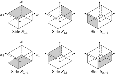
Figure 1: Convention for the sides of $R_{T}=[0,T]\times R$.

We consider a time-homogeneous diffusion process $(X_{t})_{t\geq 0}$ living in $R$. On each side of $R$, the process $X$ may be reflected or absorbed. Moreover, if $T<+\infty$, the process is stopped at time $T$. We can thus identify the sides of $R$ with the sides $S_{i,\eta}$ of $R_{T}$ for $i\in\{1,2\}$ and $\eta\in\{-1,1\}$. We denote by $\mathfrak{R}$ the subset of $\{1,2\}\times\{-1,1\}$ that contains the indices of the sides on which a Neumann boundary condition holds (possibly, $\mathfrak{R}=\varnothing$). On this set the diffusion is reflected. Let us denote by $\mathfrak{D}$ the subset of $\{1,2\}\times\{-1,1\}$ that contains the indices of the sides on which a Dirichlet boundary condition holds. On this set the diffusion is killed. Finally let us set $\mathfrak{A}=\mathfrak{D}$ if $T=+\infty$ and $\mathfrak{A}=\{(0,1)\}\cup\mathfrak{D}$ if $T<+\infty$. With this notation the time–space process $t\mapsto(t,X_{t})$ is absorbed when hitting one of the sides $S_{i,\eta}$ with $(i,\eta)\in\mathfrak{A}$.

Let $B=(B^{1},B^{2})$ be a two-dimensional Brownian motion and $\mu=(\mu_{1},\mu_{2})$ a vector of $\mathbb{R}^{2}$. For $i\in\{1,2\}$, we set

$$\gamma_{i,\eta}=\cases{1,&\quad if $(i,\eta)\in\mathfrak{R}\mbox{ (reflection)}$,\cr 0,&\quad if $(i,\eta)\in\mathfrak{A}\mbox{ (absorption)}$.}$$

We consider the two-dimensional diffusion process $(X,\mathbb{P}_{x})_{x\in R}$ whose coordinates are, for $x=(x_{1},x_{2})\in R$,

$$X_{t}^{i}=x_{i}+B^{i}_{t}+\mu_{i}t+\gamma_{i,1}\ell_{t}^{L_{i}}(X^{i})-\gamma_{i,-1}\ell_{t}^{-L_{i}}(X^{i}),\qquad\mathbb{P}_{x}\mbox{-a.s.},$$ (2)

where $\ell_{t}^{\pm L_{i}}(X^{i})$ stands for the symmetric local time of $X^{i}$ at $\pm L_{i}$, respectively.

We define $\tau_{0}=T$, $\tau_{i}=\inf\{t>0||X_{t}^{i}|>L_{i}\}$ for $i\in\{1,2\}$ and

$$\tau=\min_{i\in\{0,1,2\}}\tau_{i}.$$

In addition, we set $J=\arg\min_{i\in\{0,1,2\}}\tau_{i}$. With this notation, unless $J\not=0$, the $J$th component of $X$ is the first to exit from the domain. For $J\in\{1,2\}$, let us define $\varepsilon=X_{\tau_{J}}^{J}/L_{J}\in\{-1,1\}$. For $J=0$ we set $\varepsilon=1$. In this case $X$ has not reached the sides of $\mathfrak{D}$ before time $T$.

The couple $(J,\varepsilon)$ labels the side in $\mathfrak{A}$ of the parallelepiped $R_{T}=[0,T]\times R$ that the diffusion $X$ hits first. Note that with our convention, the sides on which the process is reflected cannot be reached so that $\tau_{i}=+\infty$ if $X^{i}$ is reflected both at $-L_{i}$ and $L_{i}$.

We are interested in computing $\mathbb{E}_{x}[f(\tau,X_{\tau})]$ by a Monte Carlo method for a bounded, measurable function $f$ where $\tau$ is defined as above.

Instead of simulating $(\tau,X_{\tau})$, we will simulate some random variables according to the following procedure. The aim is to simulate $(J,\varepsilon,\tau,X_{\tau})$ by using an importance sampling technique. In order to do this we choose a probability $\widehat{\mathbb{P}}_{x}$ which is absolutely continuous with respect to $\mathbb{P}_{x}$, and we draw a realization of $(J,\varepsilon,\tau,X_{\tau})$. Let us set

$$\alpha_{i,\eta}=\widehat{\mathbb{P}}_{x}[(J,\varepsilon)=(i,\eta)]$$

for $(i,\eta)\in\mathfrak{A}$. For $(i,\eta)\in\mathfrak{A}$ let $k_{i,\eta}$ denote the density under $\widehat{\mathbb{P}}_{x}$ of $(\tau,X_{\tau})$ given $\{(\tau,X_{\tau})\in S_{i,\eta}\}$.

In order to simplify notation let us consider an underlying probability space $(\Omega,\mathcal{{F}},\mathbb{P}_{x})$ rich enough. Let $Z$ be a random variable on this space, with distribution $\mathbb{P}_{x}$. Let $A$ be a measurable event on this space. We suppose that, conditionally on $A$, $Z$ has a density $p(\cdot|A)$ with respect to the Lebesgue measure. Let us introduce the following convention:

$$\mathbb{P}_{x}[Z=z;A]=p(z|A)\mathbb{P}_{x}[A].$$

That is, for $B$ a measurable event of $(\Omega,\mathcal{{F}},\mathbb{P}_{x})$,

$$\mathbb{P}_{x}[\{Z\in B\}\cap A]=\int_{B}p(z|A)\mathbb{P}_{x}[A]\,{d}z=\int_{B}\mathbb{P}_{x}[Z=z;A]\,{d}z.$$

Consider now the following notation: let $(i,\eta)\in\mathfrak{A}$. For $i\in\{1,2\}$ set $j=3-i$. Then for any $\theta>0$ and $z\in S_{i,\eta}$, we define

$$M_{i,\eta}(\theta,z)=\frac{\mathbb{P}_{x}[\tau_{i}=\theta;X^{i}_{\tau_{i}}=\eta L_{i}]\mathbb{P}_{x}[X^{j}_{\theta}=z_{j};\tau_{j}>\theta]}{\alpha_{i,\eta}k_{i,\eta}(\theta,z)},$$ (3)

where $k_{i,\eta}$ is the $\{X_{\tau}\in S_{i,\eta}\}$-conditional density under $\widehat{\mathbb{P}}_{x}$ of $(\tau,X_{\tau})$.

If $T<+\infty$, we define

$$M_{0,1}(T,z)=\frac{1}{\alpha_{0,1}k_{0,1}(T,z)}\prod_{j\in\{1,2\}}\mathbb{P}_{x}[X^{j}_{T}=z_{j};\tau_{j}>T],$$ (4)

where $k_{i,\eta}$ is the $\{X_{\tau}\in S_{i,\eta}\}$-conditional density under $\widehat{\mathbb{P}}_{x}$ of $(\tau,X_{\tau})$.

We call $M_{i,\eta}$ weight.

Proposition 1

The weights $M_{i,\eta}$ defined in $(\ref{eq-weight-1})$ and $(\ref{eq-weight-2})$ satisfy

$$\mathbb{E}_{x}[f(\tau,X_{\tau})]=\widehat{\mathbb{E}}_{x}[M_{J,\varepsilon}(\tau,X_{\tau})f(\tau,X_{\tau})]$$

for any measurable and bounded function $f$ on $\partial R_{T}$.

Before proving this proposition let us introduce the algorithm.

The algorithm is described as follows:

Algorithm 1.

Let $x$ be fixed in $R$.

1. [(1)]

2. Draw a realization $(\overline{J},\overline{\varepsilon})$ of $(J,\varepsilon)\in\mathfrak{A}$ under $\widehat{\mathbb{P}}_{x}$.

3. Draw a realization of the exit time and exit position $(\overline{\tau},\overline{X}_{\overline{\tau}})$ according to the density $k_{\overline{J},\overline{\varepsilon}}$ on $S_{\overline{J},\overline{\varepsilon}}$.

4. Compute the value of $M_{\overline{J},\overline{\varepsilon}}(\overline{\tau},\overline{X}_{\overline{\tau}})$ by

   $$\widehat{\mathbb{E}}_{x}[M_{J,\varepsilon}(\tau,X_{\tau})f(\tau,X_{\tau})]=\mathbb{E}_{x}[f(\tau,X_{\tau})].$$

   We call $M_{\overline{J},\overline{\varepsilon}}(\overline{\tau},\overline{X}_{\overline{\tau}})$, weight.

If $\{(\overline{J}^{(i)},\overline{\varepsilon}^{(i)},\overline{\tau}^{(i)},\overline{X}_{\overline{\tau}}^{(i)},\overline{w}^{(i)})\}_{i=1,\ldots,N}$ are $N$ independent realizations of the random variables $(J,\varepsilon,\tau,X_{\tau},M_{J,\varepsilon}(\tau,X_{\tau}))$ constructed as above, by the law of large numbers we have

$$\mathbb{E}_{x}[f(\tau,X_{\tau})]=\lim_{N\to\infty}\frac{1}{N}\sum_{i=1}^{N}\overline{w}^{(i)}f\bigl{(}\overline{\tau}^{(i)},\overline{X}_{\overline{\tau}^{(i)}}^{(i)}\bigr{)}.$$

The main feature of our approach is that the weights $M_{J,\varepsilon}(\tau,X_{\tau})$ can be easily evaluated.

Remark 1.

In order to evaluate $M_{i,\eta}$ with (3) and (4), there is no need to know $\mathbb{P}_{x}[(J,\varepsilon)=(i,\eta)]$. It is important to notice that $M_{i,\eta}$ depends only on the one-dimensional distributions of the drifted Brownian motion.

Proof of the Proposition 1 We want to prove that

$$\mathbb{E}_{x}[f(\tau,X_{\tau})]=\widehat{\mathbb{E}}_{x}[M_{J,\varepsilon}(\tau,X_{\tau})f(\tau,X_{\tau})]$$

for any measurable and bounded function $f$ on $\partial R_{T}$.

We remark first that if $p_{i,\eta}=\mathbb{P}_{x}[(J,\varepsilon)=(i,\eta)]$ for $(i,\eta)$ in $\mathfrak{A}$, then

$$\mathbb{E}_{x}[f(\tau,X_{\tau})]=\sum_{(i,\eta)\in\mathfrak{A}}\frac{p_{i,\eta}}{\alpha_{i,\eta}}\widehat{\mathbb{E}}_{x}[M_{i,\eta}(\tau,X_{\tau})f(\tau,X_{\tau})|(J,\varepsilon)=(i,\eta)].$$ (5)

Furthermore, for $(i,\eta)\in\mathfrak{D}$, if $i=2$ set $j=1$ and $z=(z_{1},\eta L_{2})$ else, if $i=1$ set $j=2$ and $z=(\eta L_{1},z_{2})$.

$$\mathbb{E}_{x}[f(\tau,X_{\tau})|(J,\varepsilon)=(i,\eta)]$$

$$\qquad=\int_{[0,T]\times[-L_{j},L_{j}]}f(\theta,z)\mathbb{P}_{x}[(\tau_{i},X^{j}_{\tau_{i}})=(\theta,z_{j})|(J,\varepsilon)=(i,\eta)]\,{d}\theta\,{d}z_{j},$$

where $\mathbb{P}_{x}[(\tau_{i},X^{j}_{\tau_{i}})=(\theta,z_{j})|(J,\varepsilon)=(i,\eta)]$ is the $\{(J,\varepsilon)=(i,\eta)\}$-conditional density of $(\tau_{i},X^{j}_{\tau_{i}})$ with respect to ${d}t\,{d}z_{j}$. Hence

$$\mathbb{E}_{x}[f(\tau,X_{\tau})|(J,\varepsilon)=(i,\eta)]=\widehat{\mathbb{E}}_{x}[f(\tau,X_{\tau})M^{\prime}_{i,\eta}(\tau,X_{\tau})|(J,\varepsilon)=(i,\eta)],$$

where

$$M_{i,\eta}^{\prime}(\theta,z)=\frac{\mathbb{P}_{x}[(\tau_{i},X^{j}_{\tau_{i}})=(\theta,z_{j})|(J,\varepsilon)=(i,\eta)]}{k_{i,\eta}(\tau,X_{\tau})}.$$

Let us note that $M_{i,\eta}(\theta,z)=M^{\prime}_{i,\eta}(\theta,z)p_{i,\eta}/\alpha_{i,\eta}$. With (5), we can deduce that

$$\mathbb{E}_{x}[f(\tau,X_{\tau})]=\widehat{\mathbb{E}}_{x}[f(\tau,X_{\tau})M_{J,\varepsilon}(\tau,X_{\tau})].$$

Indeed, it suffices to remark that for $(i,\eta)\in\mathfrak{D}$,

$$M_{i,\eta}(\theta,z) = \frac{1}{\alpha_{i,\eta}k_{i,\eta}(\theta,z)}\mathbb{P}_{x}[(\tau_{i},X^{j}_{\tau_{i}})=(\theta,z_{j});(J,\varepsilon)=(i,\eta)]$$

$$= \frac{1}{\alpha_{i,\eta}k_{i,\eta}(\theta,z)}\mathbb{P}_{x}[(\tau_{i},X^{j}_{\tau_{i}})=(\theta,z_{j});X^{i}_{\tau_{i}}=\eta L_{i},\tau^{j}>\theta].$$

The independence of the coordinates of $X$ leads to the desired equality. If $T<+\infty$, similar computations imply that for $z\in R$,

$$M_{0,1}(T,z)=\frac{1}{\alpha_{0,1}k_{0,1}(T,z)}\mathbb{P}_{x}\Bigl{[}X_{T}=z;\min_{i\in\{1,2\}}\tau_{i}>T\Bigr{]}$$

and the conclusion also holds.

Let us evaluate these probabilities.

For $i\in\{1,2\}$, let $p^{i}(t,x_{1},x_{2})$ be the solution of

$$\cases{\displaystyle\frac{\partial p^{i}(t,x_{1},x_{2})}{\partial t}=\frac{1}{2}\,\frac{\partial^{2}p^{i}}{\partial x_{2}^{2}}(t,x_{1},x_{2})+\mu_{i}\,\frac{\partial p^{i}}{\partial x_{2}}(t,x_{1},x_{2}),\cr\hskip 134.2pt\mbox{for }\displaystyle(t,x_{1},x_{2})\in\mathbb{R}_{+}\times(-L_{i},L_{i})^{2},\cr p^{i}(t,x_{1},x_{2})\mathop{\longrightarrow}\limits_{t\searrow 0}\delta_{x_{1}}(x_{2}),\qquad\mbox{for $(x_{1},x_{2})\in(-L_{i},L_{i})^{2}$},}$$ (6)

with the following boundary conditions (b.c.):

$$p^{i}(t,x_{1},-L_{i}) = 0\mbox{ (Dirichlet b.c.)}\qquad\mbox{if }(i,-1)\in\mathfrak{A},$$

$$\frac{\partial p^{i}}{\partial x_{2}}(t,x_{1},-L_{i}) = 0\mbox{ (Neumann b.c.)}\qquad\mbox{if }(i,-1)\in\mathfrak{R},$$

$$p^{i}(t,x_{1},L_{i}) = 0\mbox{ (Dirichlet b.c.)}\qquad\mbox{if }(i,1)\in\mathfrak{A},$$

$$\frac{\partial p^{i}}{\partial x_{2}}(t,x_{1},L_{i}) = 0\mbox{ (Neumann b.c.)}\qquad\mbox{if }(i,1)\in\mathfrak{R}.$$

Thus, $p^{i}$ denotes the density of the drifted Brownian motion $X^{i}$ with possibly some reflection at the endpoints of $(-L_{i},L_{i})$, and killed when it exits from this interval by an endpoint where no reflection holds. For $f$ a bounded measurable function from $[-L_{i},L_{i}]$ to $\mathbb{R}$, we have

$$\mathbb{E}_{x_{1}}[f(X^{i}_{t});t<\tau_{i}]=\int_{-L_{i}}^{L_{i}}p^{i}(t,x_{1},x_{2})f(x_{2})\,{d}x_{2}$$

for $x_{1}\in[-L_{i},L_{i}]$ where $\mathbb{P}_{x_{1}}$ is the distribution of $X^{i}$ with $X^{i}_{0}=x_{1}\in[-L_{i},L_{i}]$. Let us note that the distribution of the marginal $X^{i}$ of $X$ under $\mathbb{P}_{(x_{1},x_{2})}$ depends only on $x_{i}$.

We introduce the scale function $\Phi^{i,+}$ of $X^{i}$ defined by

$$\mbox{for $x_{2}\in[-L_{i},L_{i}]$,}\qquad\Phi^{i,+}(x_{2})=\cases{\displaystyle\frac{e^{2\mu_{i}L_{i}}-e^{-2\mu_{i}x_{2}}}{e^{2\mu_{i}L_{i}}-e^{-2\mu_{i}L_{i}}},&\quad if $\mu_{i}\not=0$,\cr\displaystyle\frac{x_{2}+L_{i}}{2L_{i}},&\quad if $\mu_{i}=0$.}$$

The function $\Phi^{i,+}(x_{2})$ has been normalized such that $\Phi^{i,+}(L_{i})=1$. Let us note that $\Phi^{i,+}(x_{i})=\mathbb{P}_{x_{i}}[X^{i}_{\tau_{i}}=L_{i}]$ if Dirichlet boundary conditions hold at both endpoints $-L_{i}$ and $L_{i}$. We also set $\Phi^{i,-}(x_{2})=1-\Phi^{i,+}(x_{2})$.

If Dirichlet boundary conditions hold both at $-L_{i}$ and $L_{i}$, then we set for $t>0$ and $(x_{1},x_{2})\in[-L_{i},L_{i}]^{2}$,

$$p^{i,\pm}(t,x_{1},x_{2})=p^{i}(t,x_{1},x_{2})\frac{\Phi^{i,\pm}(x_{2})}{\Phi^{i,\pm}(x_{1})}.$$

Via a Doob transform, for a bounded and measurable function $f$,

$$\mathbb{E}_{x_{1}}[f(X_{t}^{i});t<\tau_{i}|X^{i}_{\tau_{i}}=\pm L_{i}]=\int_{-L_{i}}^{L_{i}}p^{i,\pm}(t,x_{1},x_{2})f(x_{2})\,{d}x_{2}.$$

Let us set for $x_{1}\in(-L_{i},L_{i})$,

$$q^{i}(t,x_{1})=-\int_{-L_{i}}^{L_{i}}\frac{\partial p^{i}}{\partial t}(t,x_{1},x_{2})f(x_{2})\,{d}x_{2}$$ (7)

and

$$q^{i,\pm}(t,x_{1})=-\int_{-L_{i}}^{L_{i}}\frac{\partial p^{i,\pm}}{\partial t}(t,x_{1},x_{2})f(x_{2})\,{d}x_{2}.$$ (8)

We can easily deduce that

$$\mathbb{P}_{x_{1}}[\tau_{i}\leq t]=\int_{0}^{t}q^{i}(s,x_{1})\,{d}s\quad\mbox{and}\quad\mathbb{P}_{x_{1}}[\tau_{i}\leq t|X^{i}_{\tau_{i}}=\pm L_{i}]=\int_{0}^{t}q^{i,\pm}(s,x_{1})\,{d}s.$$

In other words, $q^{i}(t,x_{1})$ [respectively, $q^{i,\pm}(t,x_{1})$] is the density of the first exit time from $[-L_{i},L_{i}]$ for $X^{i}$ (respectively, the first exit time from $[-L_{i},L_{i}]$ for $X^{i}$ given $\{X^{i}_{\tau_{i}}=\pm L_{i}\}$).

Thanks to these expressions, $M_{0,1}(T,z)$ and $M_{i,\eta}(\theta,z)$ are easily computed since

$$\mathbb{P}_{x_{i}}[X^{i}_{\theta}=z_{i};\tau_{i}>T] = p^{i}(\theta,x_{i},z_{i}),$$

$$\mathbb{P}_{x_{i}}[\tau_{i}=\theta;X^{i}_{\theta}=\pm L_{i}] = q^{i,\pm}(\theta,x_{i})\Phi^{i,\pm}(x_{i})\qquad\mbox{if }(i,-1)\in\mathfrak{A}\mbox{ and }(i,1)\in\mathfrak{A},$$

$$\mathbb{P}_{x_{i}}[\tau_{i}=\theta;X^{i}_{\theta}=L_{i}] = q^{i}(\theta,x_{i})\qquad\mbox{if }(i,-1)\in\mathfrak{R}\mbox{ and }(i,1)\in\mathfrak{A},$$

$$\mathbb{P}_{x_{i}}[\tau_{i}=\theta;X^{i}_{\theta}=-L_{i}] = q^{i}(\theta,x_{i})\qquad\mbox{if }(i,-1)\in\mathfrak{A}\mbox{ and }(i,1)\in\mathfrak{R}.$$

3 Analytical expressions for the densities

In order to compute $p^{i}(t,x_{1},x_{2})$, together with $q^{i}(t,x_{1})$ and $q^{i,\pm}(t,x_{1})$ by (7) and (8), one has to solve equation (6). By using a scaling principle, we may assume that $L_{i}=1$, as

$$p^{i}(t,x_{1},x_{2})=\frac{1}{L_{i}}p\biggl{(}\frac{t}{L_{i}^{2}},\frac{x_{1}}{L_{i}},\frac{x_{2}}{L_{i}};L_{i}\mu\biggr{)},$$

where $p(t,x_{1},x_{2};\delta)$ is solution to (6) with $L_{i}=1$ and a convective term $\mu_{i}$ equal to $\delta$.

There are basically two ways to obtain $p(t,x_{1},x_{2};\delta)$. The first one is based on the spectral expansion of $\frac{1}{2}\triangle+\delta\nabla$ since this operator may be reduced to a self-adjoint one with respect to the scalar product induced by the measure $\exp(-2\delta x_{1})$. The second one is the method of images when $\delta=0$.

If $\delta\not=0$, the case of a Dirichlet boundary condition at both endpoints may be treated by using a simple transform that reduces the problem to $\delta=0$.

For the case of Neumann boundary condition at both endpoints, one can invert term by term the Laplace transform of a series for the Green function.

In the case of a mixed boundary condition, the previous method gives rise to a series that cannot be used in practice, so only the spectral expansion should be used. In addition, the first eigenvalues have to be computed numerically.

As the formula are standard in most of the cases, we give the relevant expressions in the Appendix.

4 General domain

As stated before, we aim to solve by a Monte Carlo method a parabolic or an elliptic PDE. The idea is to represent the domain as the union of time–space parallelepipeds and to simulate the successive exit times and positions from these parallelepipeds. Attention has to be paid while doing this decomposition in order to control the error at each simulation step.

4.1 From parallelepipeds to right parallelepipeds

Consider herein the notation of Section 2. Let us study first the parabolic PDE with constant coefficients $\lambda$, $c$ and $\mu=(\mu_{i})_{i=1,\ldots,d}$ on the rectangle $R_{T}$,

$$\qquad\cases{\displaystyle\frac{\partial v(t,x)}{\partial t}+\frac{1}{2}\sum_{i=1}^{d}\frac{\partial^{2}v(t,x)}{\partial x_{i}^{2}}\cr\qquad{}+\displaystyle\sum_{i=1}^{d}\mu_{i}\,\frac{\partial v(t,x)}{\partial x_{i}}+cv(t,x)=\lambda,&\quad on $R_{T}$,\cr\dfrac{\partial v(t,x)}{\partial x_{i}}=0,&\quad for $x\in S_{i,\eta}\mbox{ if }(i,\eta)\in\mathfrak{R}$,\cr v(t,x)=\phi(t,x),&\quad for $x\in S_{i,\eta}\mbox{ if }(i,\eta)\in\mathfrak{A}$,\cr v(T,x)=g(x),&\quad if $T<+\infty$.}$$ (9)

We assume that a classical solution to this problem exists, which is, for example, the case if $\phi$ and $g$ are continuous and bounded. Let $X$ be the diffusion process whose components are given by (2). Then it follows from the Itô formula applied to $X$ that, for $t\in[0,T]$,

$$v(t,x) = \mathbb{E}_{x}\bigl{[}e^{c(\tau-t)}\phi(\tau-t,X_{\tau-t});\tau<T-t\bigr{]}$$

$${}+\mathbb{E}_{x}\bigl{[}e^{c(T-t)}g(X_{T-t});\tau=T-t\bigr{]}+\mathbb{E}_{x}\biggl{[}\lambda\int_{0}^{\tau-t}e^{c(\tau-t-s)}\,{d}s\biggr{]},$$

where $\tau$ is as above the first exit time from $R_{T}$.

Let us remark that if $\sigma$ is an invertible $d\times d$-matrix, then the function $u(t,x)=v(t,\sigma^{-1}x)$ is solution to

$$\cases{\displaystyle\frac{\partial u(t,x)}{\partial t}+\frac{1}{2}\sum_{i,j=1}^{d}[\sigma{\sigma}^{*}]_{i,j}\,\frac{\partial^{2}u(t,x)}{\partial x_{i}\,\partial x_{j}}\cr\qquad{}+\displaystyle\sum_{i=1}^{d}[\mu{\sigma}^{*}]_{i}\,\frac{\partial u(t,x)}{\partial x_{i}}+cu(t,x)=\lambda,\cr\hskip 119.08pt\mbox{on $[0,T]\times\sigma R$},\cr\sigma_{j,i}\,\dfrac{\partial u(t,x)}{\partial x_{j}}=0,\qquad\hskip 17.7pt\mbox{for $x\in\sigma S_{i,\eta}$ if $(i,\eta)\in\mathfrak{R}$},\cr u(t,x)=\phi(t,\sigma^{-1}x),\qquad\mbox{for $x\in\sigma S_{i,\eta}$ if $(i,\eta)\in\mathfrak{A}$},\cr u(T,x)=g(\sigma^{-1}x),\qquad\hskip 7.09pt\mbox{if $T<+\infty$.}}$$ (10)

If $\mathbf{n}_{i}$ is the unit vector orthogonal to the side $\sigma S_{i,\eta}$, then $\mathbf{n}_{i}=({\sigma}^{*})^{-1}\mathbf{e}_{i}$, where $\mathbf{e}_{i}$ is the unit vector in the $i$th direction. It follows that $\sigma{\sigma}^{*}\mathbf{n}_{i}=\sigma\mathbf{e}_{i}$ and thus

$$\mbox{for }x\in\sigma S_{i,\pm 1}\qquad[\sigma{\sigma}^{*}]\mathbf{n}_{i}\cdot\nabla u(t,x)=\sigma_{j,i}\,\frac{\partial u(t,x)}{\partial x_{j}},$$

which means that a Neumann boundary condition in the co-normal direction holds in (10) on $\sigma S_{i,\eta}$ if $(i,\eta)\in\mathfrak{R}$.

We can thus solve (10) by reducing the problem to (9) and use a Monte Carlo method in order to compute the values of $u(t,x)$.

4.2 The hypotheses

Let us consider a domain $Q$ in $\mathbb{R}_{+}\times\mathbb{R}^{d}$. For the sake of simplicity, we assume that $Q$ is the cylinder $[0,T]\times D$ (with possibly $T=+\infty$), where $D$ is an open, bounded domain of $\mathbb{R}^{d}$ with piecewise smooth boundary. Let us consider a function $a$ with values in the space of $d\times d$-symmetric matrices which is continuous on $D$ and everywhere positive definite, together with some functions $b\dvtx Q\to\mathbb{R}^{d}$, $c\dvtx Q\to\mathbb{R}$ and $f\dvtx Q\to\mathbb{R}$. For all $(t,x)\in Q$, we denote by $\sigma(t,x)$ a $d\times d$-symmetric matrix such that $\sigma(t,x){\sigma}^{*}(t,x)=a(t,x)$.

We set

$$L=\frac{1}{2}\sum_{i,j=1}^{d}a_{i,j}(t,x)\,\frac{\partial^{2}}{\partial x_{i}\,\partial x_{j}}+\sum_{i=1}^{d}b_{i}(t,x)\,\frac{\partial}{\partial x_{i}}.$$

Let us introduce the hypotheses needed to ensure the convergence of our algorithm. To set up a Monte Carlo numerical scheme, one needs three inter-connected ingredients:

The existence and the uniqueness of a solution $u$ to the following PDE

$$\cases{\dfrac{\partial u(t,x)}{\partial t}+Lu(t,x)\cr\qquad{}+c(t,x)u(t,x)+f(t,x)=0,&\quad on $[0,T]\times D$,\cr u(T,x)=g(x),&\quad$x\in D$,\cr u(t,x)=\phi(t,x),&\quad on $\Gamma_{\mathrm{d}}\subset[0,T)\times\partial D$,\cr\partial_{n}u(t,x)=0,&\quad on $\Gamma_{\mathrm{n}}\subset[0,T)\times\partial D$,}$$ (11)

where $\partial_{n}$ denotes the co-normal derivative along the lateral surface. $\Gamma_{\mathrm{d}}$ (respectively, $\Gamma_{\mathrm{n}}$) are subsets of $[0,T)\times\partial D$ on which a Dirichlet (respectively, Neumann) boundary condition holds.

The existence of a solution to the diffusion process associated with $L$. Note that since the simulation involves distributions and not stochastic integrals, we do not need strong existence for the associated SDE.

The solution $u$ can be expressed in terms of the probabilistic representation

$$u(t,x) = \mathbb{E}_{t,x}\biggl{[}\exp\biggl{(}\int_{t}^{\tau}c(s,X_{s})\,{d}s\biggr{)}\phi(\tau,X_{\tau})\mathbh{1}_{\tau<T}\biggr{]}$$

$${}+\mathbb{E}_{t,x}\biggl{[}\exp\biggl{(}\int_{t}^{T}c(s,X_{s})\,{d}s\biggr{)}g(X_{T})\mathbh{1}_{\tau>T}\biggr{]}$$

$${}+\mathbb{E}_{t,x}\biggl{[}\int_{t}^{\tau\wedge T}\exp\biggl{(}\int_{t}^{s}c(r,X_{r})\,{d}r\biggr{)}f(s,X_{s})\,{d}s\biggr{]},$$

where $\tau$ is the first exit time from $[0,+\infty)\times D$ by a point of $\Gamma_{\mathrm{d}}$.

Notation 1.

We denote by $\mathcal{P}$ the set of time–space parallelepipeds $P$ such that there exist $0\leq s<t\leq T$, $L_{1},\ldots,L_{d}$ and $x\in\mathbb{R}^{d}$ such that

$$P=[s,t]\times\bigl{(}x+\widehat{\sigma}([-L_{1},L_{1}]\times\cdots\times[-L_{d},L_{d}])\bigr{)},$$

where $\widehat{\sigma}$ is a $d\times d$-matrix. Possibly $t=+\infty$ (if $T=+\infty$).

The assumptions that have to be done are the following:

1. [(H1)]

2. There exists a subset $\mathcal{P}_{D}$ of $\mathcal{P}$ such that $Q=\bigcup_{P\in\mathcal{P}_{D}}P$. Besides, if $P=[s,t]\times U\in\mathcal{P}$ for a parallelepiped $U$, then for all $r\in[s,t)$, $[r,t]\times U\in\mathcal{P}$. In other words, one can truncate the parallelepipeds in time.

3. There exist $\Gamma_{\mathrm{n}}$, $\Gamma_{\mathrm{d}}$ contained in $\partial Q=[0,T]\times\partial D$ and some subsets $\mathcal{P}_{\mathrm{n}}$, $\mathcal{P}_{\mathrm{d}}$ of $I$ such that $\Gamma_{\mathrm{n}}\subset\bigcup_{P\in\mathcal{P}_{\mathrm{n}}}\partial P$, $\Gamma_{\mathrm{d}}\subset\bigcup_{P\in\mathcal{P}_{\mathrm{d}}}\partial P$. The closure of $\Gamma_{\mathrm{n}}\cup\Gamma_{\mathrm{d}}$ is equal to $[0,T]\times\partial D$ and $\Gamma_{\mathrm{n}}\cap\Gamma_{\mathrm{d}}=\varnothing$. This means that the boundary of $[0,T]\times\partial D$ is split in two distinct parts, where either the Dirichlet or the Neumann boundary conditions hold. More precisely a side of a parallelepiped in $\mathcal{P}_{D}$ contained in $\partial Q$ is either from $\Gamma_{\mathrm{n}}$ or from $\Gamma_{\mathrm{d}}$.

4. The differential operator $L$ is the generator of a continuous diffusion process $X$ that is reflected at $\Gamma_{\mathrm{n}}$ and killed when hitting $\Gamma_{\mathrm{d}}\cup\{T\}\times D$. The probabilistic representation of the solution given by (4.2) holds (see, e.g., lions84a for existence results of such reflected process and stroock79a if there are no reflections).

5. There exists an unique solution $u$ of class $\mathcal{C}^{1,2}$ on $[0,T)\times D$ to (11) which is continuous on $[0,T]\times\overline{D}$.

6. For a right parallelepiped $R$ and a matrix $\widehat{\sigma}$ let $P=[s,t]\times(x+\widehat{\sigma}R)\in\mathcal{P}_{D}$. We associate with $P$ a vector $\widehat{b}\in\mathbb{R}^{d}$, two constants $\widehat{c}$, $\widehat{f}$ and we construct the differential operator

   $$\widehat{L}=\frac{1}{2}\sum_{k,l=1}^{d}\widehat{a}_{k,\ell}\,\frac{\partial^{2}}{\partial x_{k}\,\partial x_{\ell}}+\sum_{k=1}^{d}\widehat{b}_{k}\,\frac{\partial}{\partial_{x_{k}}}$$

   with $\widehat{a}=\widehat{\sigma}{\widehat{\sigma}}^{*}$.

   Fix $\delta>0$. We assume that the solution $u$ to (11) satisfies, for any $y$ in the interior of $x+\widehat{\sigma}R$,

   $$\mathbb{E}_{s,y}\biggl{|}\int_{s}^{\tilde{\tau}}e^{\widehat{c}(r-s)}\biggl{(}\frac{\partial u}{\partial t}+\widehat{L}u+\widehat{c}u-\widehat{f}\biggr{)}(r,\widehat{X}_{r})\,{d}r\biggr{|}\leq\delta,$$

   where $\widehat{X}$ is the diffusion process generated by $\widehat{L}$, and ${\tilde{\tau}}$ is its first exit time from $P$.

Remark 2.

If $T=+\infty$ and the coefficients are time-homogeneous and $\Gamma_{\mathrm{d}}=[0,\infty)\times\gamma_{\mathrm{d}}$, $\Gamma_{\mathrm{n}}=[0,\infty)\times\gamma_{\mathrm{n}}$, then $v(x)=u(0,x)$ is solution to the elliptic PDE

$$\cases{Lv(x)+c(x)v(x)=f(x),&\quad on $D$,\cr v(x)=\phi(x),&\quad on $\gamma_{\mathrm{d}}\subset\partial D$,\cr\partial_{n}v(x)=0,&\quad on $\gamma_{\mathrm{n}}\subset\partial D$.}$$ (13)

Thus, by solving the parabolic PDE (11), we may also solve the elliptic PDE (13). We will thus focus only on (11).

Remark 3.

The result of the existence of a stochastic process reflected on some part of the boundary of $[0,T)\times D$ is deduced from the existence of a stochastic process reflected on the lateral boundary $[0,T)\times D$ which is killed when it hits $\Gamma_{\mathrm{n}}$.

4.3 The algorithm and its weak error

In order to simplify the notation, if $T<+\infty$, we denote the final condition $g$ of (11) by $\phi(T,x)$.

Given $(t,x)\in Q$, the solution $u(t,x)$ of (11) is computed by the Feynman–Kac formula. For this, we have to simulate the diffusion process $X$ up to its first exit time $\tau$ from $Q$. We suppose here that the particle cannot exit by a part of boundary where a Neumann boundary condition holds. Let $u$ be the solution of (11). Let us introduce the following notation:

$$\mbox{for }s\geq t\qquad\cases{\displaystyle Y_{s}=1+\int_{t}^{s}c(r,X_{r})Y_{r}\,{d}r=\exp\biggl{(}\int_{t}^{s}c(r,X_{r})\,{d}r\biggr{)},\cr\displaystyle Z_{s}=\int_{t}^{s}f(r,X_{r})Y_{r}\,{d}r.}$$

Then $u(t,x)$ is given by

$$u(t,x)=\mathbb{E}_{t,x}[\phi(\tau,X_{\tau})Y_{\tau}+Z_{\tau}].$$ (14)

We construct now the algorithm that approximates (14) by a Monte Carlo method.

Algorithm 2.

Assume that we start initially at the point $(t,x)\in Q$ and fix a number $N$ of particles.

1. [(1)]

2. For $i=1,\ldots,N$ do

   1. [(A)]

   2. Set $(\theta_{0},\Xi_{0},Y_{0},Z_{0},W_{0})=(t,x,1,0,1)$ and $k=0$.

   3. Repeat:

      1. [(a)]

      2. Choose an element $P^{(k)}\in\mathcal{P}_{D}$ of the form $P^{(k)}=[\theta_{k},s]\times U$, $U\subset\mathbb{R}^{d}$ such that $(\theta_{k},\Xi_{k})$ belongs to the basis of $P$ ($s$ is possibly infinite if, for example, $T=+\infty$ and the coefficients are time-inhomogeneous). On $P^{(k)}$, consider the differential operator $L^{(k)}$ as well $c^{(k)}$ and $f^{(k)}$ which approximate $L$, $c$ and $f$ as in (H5).

      3. Draw a realization of a random variable $(\theta_{k+1},\Xi_{k+1})$ with values in $(\{s\}\times U)\cup((\theta_{k},s)\times\partial U)$ and compute its associated weight $w_{k}$ as shown in Sections 2 and 4.1 by considering the exit time and position from the parallelepiped $P^{(k)}$.

      4. Compute $W_{k}=W_{k-1}w_{k}$ and

         $$Y_{k+1} = Y_{k}\exp\bigl{(}c^{(k)}(\theta_{k+1}-\theta_{k})\bigr{)},$$

         $$Z_{k+1} = Z_{k}+f^{(k)}\int_{\theta_{k}}^{\theta_{k+1}}\exp\bigl{(}c^{(k)}s\bigr{)}\,{d}s.$$

      5. If $\Xi_{k+1}\in\Gamma_{\mathrm{d}}$ or $\theta_{k+1}=T$, then exit from the loop.

      6. Increase $k$.

   4. Set $(\theta^{(i)},\Xi^{(i)},Y^{(i)},Z^{(i)},W^{(i)})=(\theta_{k+1},\Xi_{k+1},Y_{k+1},Z_{k+1},W_{k})$.

3. Return

   $$\widehat{u}(t,x)=\frac{1}{N}\sum_{i=1}^{N}\bigl{(}W^{(i)}\phi\bigl{(}\theta^{(i)},\Xi^{(i)}\bigr{)}Y^{(i)}+W^{(i)}Z^{(i)}\bigr{)}.$$ (15)

We denote from now on by $\widehat{\mathbb{P}}_{x}$ the distribution of the Markov chain $\Lambda_{k}=(\theta_{k},\Xi_{k}),k\geq 0$. Note that $(Y_{k},Z_{k},w_{k})_{k\geq 0}$ is obtained from $(\Lambda_{k})_{k\geq 0}$.

Proposition 2

For any $(t,x)\in[0,T)\times D$,

$$|u(t,x)-\widehat{\mathbb{E}}_{x}[\widehat{u}(t,x)]|\leq\delta\widehat{\mathbb{E}}_{x}[W_{\nu}\nu\exp(M\theta_{\nu})],$$ (16)

where $\delta$ is defined in (H5), $\nu$ is the number of steps that $(\Lambda_{k})_{k\geq 0}$ takes to reach the boundary $\Gamma_{\mathrm{d}}\cap\{T\}\times D$ and

$$M=\sup_{(s,y)\in[t,T)\times D}c(s,y).$$

Remark 4.

Note that the weak error in (16) does not depend on the choice of the importance sampling technique while the Monte Carlo error depends on this choice. If the coefficients $a$, $b$, $f$ and $c$ are constant on the domain, one can choose $\delta=0$ and the simulation becomes exact.

To the Markov chain $(\Lambda_{k})_{k\geq 0}$ is associated a random sequence of parallelepipeds $(P^{(k)})_{k=0,\ldots,\nu}$. Let us denote by $\tau^{(k)}$ the successive times the diffusion process $X$ reaches the boundary of the $P^{(k)}$’s.

Since $Z_{0}=0$, $Y_{0}=1$ and $u=\phi$ on the boundary of $Q$, we get

$$\qquad\widehat{\mathbb{E}}_{x}[\widehat{u}(t,x)] = \widehat{\mathbb{E}}_{x}[W_{\nu}Y_{\nu}\phi(\theta_{\nu},\Xi_{\nu})+W_{\nu}Z_{\nu}]$$

$$= u(t,x)+\widehat{\mathbb{E}}_{x}\Biggl{[}W_{\nu}\sum_{k=0}^{\nu-1}\bigl{(}Z_{k+1}-Z_{k}+Y_{k+1}u(\theta_{k+1},\Xi_{k+1})$$

$$\hskip 177.2pt{}-Y_{k}u(\theta_{k},\Xi_{k})\bigr{)}\Biggr{]}.$$

Let $(\mathcal{G}_{k})_{k\geq 0}$ be the filtration generated by the Markov chain $(\Lambda_{k})_{k\geq 0}$. We remark that $Y_{k}$ and $Z_{k}$ are measurable with respect to $\mathcal{G}_{k}$ while $w_{k}$ is measurable with respect to $\mathcal{G}_{k+1}$ (since it is obtained from $\theta_{k}$, $\Xi_{k}$, $\theta_{k+1}$ and $\Xi_{k+1}$).

By using the Markov property, after setting $W_{k+1,\nu}=\widehat{\mathbb{E}}_{x}[w_{k+1}\cdots w_{\nu}|\mathcal{G}_{k+1}]$, we get

$$\widehat{\mathbb{E}}_{x}[W_{\nu}(Z_{k+1}-Z_{k})]$$

$$\qquad=\widehat{\mathbb{E}}_{x}\bigl{[}W_{k+1,\nu}\widehat{\mathbb{E}}_{x}[w_{k}(Z_{k+1}-Z_{k})|\mathcal{G}_{k}]W_{k-1}\bigr{]},$$

$$\widehat{\mathbb{E}}_{x}\bigl{[}W_{\nu}\bigl{(}Y_{k+1}u(\theta_{k+1},\Xi_{k+1})-Y_{k}u(\theta_{k},\Xi_{k})\bigr{)}\bigr{]}$$

$$\qquad=\widehat{\mathbb{E}}_{x}\bigl{[}W_{k+1,\nu}\widehat{\mathbb{E}}_{x}\bigl{[}w_{k}\bigl{(}Y_{k+1}u(\theta_{k+1},\Xi_{k+1})-Y_{k}u(\theta_{k},\Xi_{k})\bigr{)}|\mathcal{G}_{k}\bigr{]}W_{k-1}\bigr{]}.$$

Let us denote by $(X^{(k)},\mathbb{P}^{(k)}_{t,x})$ the process generated by the operator $L^{(k)}$ with constant coefficients $a^{(k)}$ and $b^{(k)}$ on $P^{(k)}$. Define recursively $(t^{(0)},x^{(0)})=(t,x)$ and $(t^{(k+1)},x^{(k+1)})=({\overline{\tau}}^{(k)},X^{(k)}_{{\overline{\tau}}^{(k)}})$ where ${\overline{\tau}}^{(k)}$ is, as above, the first exit time from $P^{(k)}$ for the diffusion $X^{(k)}$. Let also $f^{(k)}$ and $c^{(k)}$ be the values that approach $f$ and $c$ on $P^{(k)}$, and define also recursively $y^{(0)}=1$ and $y^{(k)}=y^{(k-1)}\exp(c^{(k)}(t^{(k+1)}-t^{(k)}))$.

By using the properties of $\widehat{\mathbb{P}}_{x}$ and the Itô formula we obtain

$$\widehat{\mathbb{E}}_{x}\bigl{[}w_{k}\bigl{(}Y_{k+1}u(\theta_{k+1},\Xi_{k+1})-Y_{k}u(\theta_{k},\Xi_{k})\bigr{)}|\mathcal{G}_{k}\bigr{]}$$

$$\qquad=y^{(k)}\mathbb{E}^{(k)}_{t^{(k)},x^{(k)}}\bigl{[}\bigl{(}e^{c^{(k)}(t^{(k+1)}-t^{(k)})}u\bigl{(}t^{(k+1)},X^{(k+1)}_{t^{(k+1)}}\bigr{)}-u\bigl{(}t^{(k)},x^{(k)}\bigr{)}\bigr{)}\bigr{]}$$

$$\qquad=y^{(k)}\mathbb{E}^{(k)}_{t^{(k)},x^{(k)}}\biggl{[}\int_{t^{(k)}}^{t^{(k+1)}}e^{c^{(k)}(s-t^{(k)})}\biggl{(}\frac{\partial}{\partial t}+L^{(k)}+c^{(k)}\biggr{)}u\bigl{(}s,X_{s}^{(k)}\bigr{)}\,{d}s\biggr{]}.$$

Also,

$$\widehat{\mathbb{E}}_{x}[w_{k}(Z_{k+1}-Z_{k})|\mathcal{G}_{k}]=y^{(k)}\mathbb{E}^{(k)}_{t^{(k)},x^{(k)}}\biggl{[}f^{(k)}\int_{t^{(k)}}^{t^{(k+1)}}e^{c^{(k)}s}\,{d}s\biggr{]}.$$

Under the hypothesis on the coefficients and the parallelepiped $P^{(k)}$ we have

$$\bigl{|}\widehat{\mathbb{E}}_{x}\bigl{[}w_{k}\bigl{(}Y_{k+1}u(\theta_{k+1},\Xi_{k+1})-Y_{k}u(\theta_{k},\Xi_{k})+Z_{k+1}-Z_{k}\bigr{)}|\mathcal{G}_{k}\bigr{]}\bigr{|}$$

$$\qquad=\biggl{|}y^{(k)}\mathbb{E}^{(k)}_{t^{(k)},x^{(k)}}\biggl{[}\int_{t^{(k)}}^{t^{(k+1)}}e^{c^{(k)}(s-t^{(k)})}$$

$$\hskip 124.0pt{}\times\biggl{(}\biggl{(}\frac{\partial}{\partial t}+L^{(k)}+c^{(k)}\biggr{)}u\bigl{(}s,X_{s}^{(k)}\bigr{)}+f^{(k)}\biggr{)}\,{d}s\biggr{]}\biggr{|}$$

$$\qquad\leq y^{(k)}\delta\leq\widehat{\mathbb{E}}_{x}[\delta w_{k}Y_{k}|\mathcal{G}_{k}],$$

since the $Y_{k}$’s (and so the $y^{(k)}$’s) are positive. Hence, from (4.3) and the Jensen inequality applied to $|\cdot|$, we obtain

$$|\widehat{\mathbb{E}}_{x}[Y_{\nu}\phi(\theta_{\nu},\Xi_{\nu})+Z_{\nu}]-\widehat{\mathbb{E}}_{x}[\widehat{u}(t,x)]|\leq\delta\widehat{\mathbb{E}}_{x}\Biggl{[}W_{\nu}\sum_{k=0}^{\nu-1}Y_{k}\Biggr{]}.$$

As $0<Y_{k}\leq e^{M\theta_{k}}$ for $k=0,\ldots,\nu$, we deduce (16).

4.4 The Monte Carlo error

In order to compute the solution $u(t,x)$ of (11), we have constructed the estimator $\widehat{u}(t,x)$ given by (15) whose variance is

$$\operatorname{Var}_{\widehat{\mathbb{P}}_{x}}\widehat{u}(t,x)=\frac{1}{N}\operatorname{Var}_{\widehat{\mathbb{P}}_{x}}\bigl{(}W_{\nu}\phi(\theta_{\nu},\Xi_{\nu})Y_{\nu}+W_{\nu}Z_{\nu}\bigr{)}.$$

The Monte Carlo error depends on this variance $s^{2}=\operatorname{Var}_{\widehat{\mathbb{P}}_{x}}\widehat{u}(t,x)$, since asymptotically for $N\to\infty$ the true mean $\widehat{\mathbb{E}}_{x}[\widehat{u}(t,x)]$ lies in the interval $[\widehat{u}(t,x)-2s,\widehat{u}(t,x)+2s]$ with a confidence of $95.4\%$.

We denote by $\widehat{\mathbb{P}}^{\mathrm{n}}$ the distribution of $(\Lambda_{k})_{k\geq 0}$ with respect to the real distribution of the exit time and position of the rectangles. In this case the weights are equal to $1$. Any event $\Phi$ measurable with respect to $(\Lambda_{k})_{k\geq 0}$ satisfies $\widehat{\mathbb{P}}^{\mathrm{n}}[\Phi]=\widehat{\mathbb{P}}_{x}[W\Phi]$.

We get thus

$$\operatorname{Var}_{\widehat{\mathbb{P}}_{x}}\bigl{(}W_{\nu}\phi(\theta_{\nu},\Xi_{\nu})Y_{\nu}+W_{\nu}Z_{\nu}\bigr{)}=\Psi+\operatorname{Var}_{\widehat{\mathbb{P}}^{\mathrm{n}}}(\widehat{u}(t,x))$$

with

$$\Psi=\widehat{\mathbb{E}}^{\mathrm{n}}\bigl{[}(W_{\nu}-1)\bigl{(}\phi(\theta_{\nu},\Xi_{\nu})Y_{\nu}+Z_{\nu}\bigr{)}^{2}\bigr{]}.$$

This shows that a good choice for the density of the exit time and position from the parallelepipeds is such that $\Psi\leq 0$ is as small as possible. By the way, reducing the variance is a difficult task and requires some automatic selection/optimization techniques, as explained in the Introduction.

In addition, the numerical experiments we performed up to now highlight another difficulty. $W_{\nu}$ may take large values, and this implies meaningless values for $\widehat{u}(t,x)$. That is why we suggest to keep track also of the empirical distribution, or at least of the variance of $W_{\nu}$.

In order to illustrate this, let us assume that the diffusion process $X$ has no drift and that for the simulation, the right parallelepipeds we use are squares centered on the particle, and consider the same density for the exit time and position. By a scaling argument, the distribution of the weight $w_{k}$ at the $k$th step does not depend on the size of the squares, so that the $w_{k}$’s are independent and identically distributed under $\widehat{\mathbb{P}}_{x}$.

Let us fix an integer $n$ such that $\nu\geq n$ a.s. (for example, the minimal number of steps needed to reach an absorbing boundary). We set $\xi^{i}=\log(w_{i})$, so that $W_{n}=\exp(\sum_{i=1}^{n}\xi^{i})$. As the $\xi^{i}$ are independent and identically distributed, let us note $S_{n}=\sum_{i=1}^{n}\xi^{i}$, then $S_{n}/\sqrt{n}$ converges to some normal random variable $\chi$ with mean $m$ and variance $s^{2}$. For $n$ large enough, the distribution of $W_{n}$ is close to the distribution of $\exp(\sqrt{n}\chi)$. We obtain, with the expression of the Laplace transform for the normal distribution, for $j\in\{1,2\}$,

$$\widehat{\mathbb{E}}_{x}[(W_{n})^{j}]\approx\mathbb{E}_{x}\bigl{[}\exp\bigl{(}j\sqrt{n}\chi\bigr{)}\bigr{]}=\exp\biggl{(}mj\sqrt{n}+n\frac{j^{2}s^{2}}{2}\biggr{)}.$$

This leads us to the following approximation:

$$\operatorname{Var}_{\widehat{\mathbb{P}}_{x}}(W_{n}) \approx \exp\bigl{(}2m\sqrt{n}+2ns^{2}\bigr{)}-\exp\biggl{(}m\sqrt{n}+\frac{n}{2}s^{2}\biggr{)}$$

$$\approx \exp(2ns^{2})\biggl{(}\exp\biggl{(}\frac{m}{\sqrt{n}}+1\biggr{)}-\exp\biggl{(}\frac{m}{2\sqrt{n}}-\frac{3n}{2}s^{2}\biggr{)}\biggr{)}$$

$$\mathop{\sim}\limits_{n\to\infty} \exp(1+2ns^{2}).$$

So, for large $n$, the variance of $W_{n}$ explodes, while $\widehat{\mathbb{E}}_{x}[W_{n}]=1$ for any $n\geq 1$.

In glynn (see also glasserman04a ), Glynn and Iglehart exhibit another argument that shows that the simulation performs badly if too many steps are used.

4.5 Population Monte Carlo

In order to overcome the explosion of the variance due to the weights one can use a population Monte Carlo method. This kind of method, also known as quantum Monte Carlo, sequential Monte Carlo, Green Monte Carlo$,\ldots$ has been used for a long time in physical simulations (see, e.g., iba for a brief survey) but also in signal theory, statistics$,\ldots.$ A probabilistic point of view is developed in the book delmoral04a of Del Moral.

In our case, instead of simulating the particles one after another, the idea is to keep track of the whole population of $N$ particles $(y^{(i)})_{i\in\{1,\ldots,N\}}$ with time and space coordinates $(t^{(i)},x^{(i)})$ and a weight $w^{(i)}$ according to the algorithm given below. Each particle has two possible states: still running or stopped. A particle is stopped either at the first time it reaches an absorbing boundary, or if its time is equal to the finite final time $T$. Otherwise, the particle is still running.

Algorithm 3.

This algorithm computes an approximation of the quantity $\mathbb{E}_{x}[f(T\wedge\tau,X_{T\wedge\tau})]$ when $X_{0}=0$ by using a population of $N$ particles.

1. Set $n=0$; $n$ is the number of steps.

2. For $i$ from $1$ to $N$ set

   1. [(a)]

   2. $(w^{(i)}_{0},t^{(i)}_{0},x^{(i)}_{0})=(0,0,x)$.

3. Set $\mathfrak{S}=\varnothing$ and $\mathfrak{R}_{n}=\{(w^{(i)}_{0},t^{(i)}_{0},x^{(i)}_{0})\}_{i=1,\ldots,N}$.

4. While the set $\mathfrak{R}_{n}$ of still running particles at step $n$ is nonempty do:

   1. [(a)]

   2. Set $\mathfrak{R}_{n+1}=\varnothing$.

   3. Do $\#\mathfrak{R}_{n}$ times the following operations:

      1. [(iii)]

      2. Pick a still running particle of index $j$ at random according to a family of discrete probability distribution

         $$p_{j}=\frac{w^{(j)}_{n}}{\sum_{k\ \mathrm{index}\ \mathrm{of}\ \mathrm{particles}\ \mathrm{in}\ \mathfrak{R}_{n}}w^{(k)}_{n}},$$

         where $w^{(j)}_{n}$ is the weight of the particle after $n$ iterations.

      3. The particle is moved in time and space according to the exit time and position from a time–space parallelepiped that contains $(t^{(j)}_{n},x^{(j)}_{n})$. Its new position is denoted $(t^{(j)}_{n+1},x^{(j)}_{n+1})$ and its associated weight $w^{(j)}_{n+1}$.

      4. If $t^{(j)}_{n+1}=T$ or if $x^{(j)}_{n+1}$ belongs to an absorbing boundary, then $(w^{(j)}_{n+1},t^{(j)}_{n+1},x^{(j)}_{n+1})$ is added to the set $\mathfrak{S}$ of stopped particles. Otherwise, it is added to $\mathfrak{R}_{n+1}$.

   4. Increment $n$ by $1$.

5. Return

   $$\frac{1}{\sum_{i=1}^{N^{\prime}}w^{(i)}}\sum_{i=1}^{N^{\prime}}w^{(i)}f\bigl{(}t^{(i)},x^{(i)}\bigr{)},$$

   when $\mathfrak{S}=\{(w^{(i)},t^{(i)},x^{(i)})\}_{i=1,\ldots,N^{\prime}}$.

As we need to keep track of the positions of all the particles, this algorithm is memory consuming. On the other hand, it avoids the multiplication of the weights. In addition, this algorithm can be modified in the following way: instead of using $\#\mathfrak{R}_{n}$ particles at step $n$, it is possible to use $N$ particles, and in this case, one has to keep track of the number of still running particles and to multiply the weights by the proportion of still running particles. The algorithm stops when the proportion of still running particles is smaller than a given threshold. This approach can be used, for example, for long time simulation, or to estimate rare events, as, for example, in cerou06a , delmoral04a , delmoral05a , lejay08a .

4.6 Estimation of the number of steps

Let us consider now the estimation of the number of steps. In order to do this we will use the techniques employed in milstein95a , milstein99a , milstein04a .

In Algorithm 2, we have constructed the Markov chain $(\Lambda_{k})_{k\geq 0}$ which is absorbed when reaching $\Gamma_{\mathrm{k}}=\Gamma_{\mathrm{d}}\cap\{T\}\times D$.

For a function $u$ on $D$, we set

$$Pu(t,x)=\widehat{\mathbb{E}}^{\mathrm{n}}[u(\Lambda_{1})|\Lambda_{0}=(t,x)]\quad\mbox{and}\quad A=Pu(t,x)-u(t,x).$$

The operator $A$ is the generator of a Markov chain.

Lemma 1.

If $T<+\infty$ and

$$\widehat{\mathbb{E}}^{\mathrm{n}}[\theta_{1}|(\theta_{0},\Xi_{0})=(t,x)]-t\geq\gamma,$$

then

$$\widehat{\mathbb{E}}^{\mathrm{n}}[\nu|(\theta_{0},\Xi_{0})=(t,x)]\leq 1+\frac{T-t}{\gamma}.$$

Consider the problem

$$\cases{Av(t,x)=-g(t,x),&\quad on $Q$,\cr u(t,x)=0,&\quad on $[0,T]\times\Gamma$,}$$

whose solution is

$$u(t,x)=\widehat{\mathbb{E}}^{\mathrm{n}}\Biggl{[}\sum_{k=0}^{\nu-1}g(\Lambda_{k})\Biggr{]}.$$

We remark that if $u$ and $g$ are well chosen this equality gives a good estimate of $\widehat{\mathbb{E}}^{\mathrm{n}}[\nu]$.

Let $V(t,x)$ be the function $V(t,x)=(T-t)\mathbh{1}_{(t,x)\in Q}$. For $(t,x)$ in $Q$, we have

$$AV(t,x)=\widehat{\mathbb{E}}^{\mathrm{n}}[V(\theta_{1},\Xi_{1})|(\theta_{0},\Xi_{0})=(t,x)]-(T-t)\leq-\gamma.$$

Hence $T-t\geq\widehat{\mathbb{E}}^{\mathrm{n}}[\sum_{k=0}^{\nu-1}\gamma|(\theta_{0},\Xi_{0})=(t,x)]$ and the result follows easily.

Lemma 2.

With the previous notation, for every $L>0$ fixed, we have

$$\sup_{x\in Q}\widehat{\mathbb{P}}^{\mathrm{n}}[\nu\geq L|(\theta_{0},\Xi_{0})=(t,x)]\leq(1+T-t)\exp\bigl{(}-c\gamma L/(1+T-t)\bigr{)},$$

where $c$ is a constant depending on $\gamma$; more precisely $c$ converges to $1$ as $\gamma$ decreases to $0$.

The proof follows from the one of Theorem 7.2 in milstein99a .

Lemma 3.

If $T=+\infty$, $Q$ is bounded and

$$\widehat{\mathbb{E}}^{\mathrm{n}}[|x+\Xi_{1}+c|^{2}]\geq\gamma>0,$$

where $c$ is such that $\min_{x\in\overline{Q}}|x+c|\geq C>0$. Then

$$\widehat{\mathbb{E}}^{\mathrm{n}}[\nu]\leq\frac{B^{2}-C^{2}}{B^{2}-\gamma}$$

with $B>\max\{\gamma,\sup_{x\in\overline{Q}}|x+c|\}$.

Let us proceed as in milstein95a . Choose a vector $c$ such that $\min_{x\in\overline{Q}}|x+c|\geq C>0$, and set

$$V(t,x)=\cases{B^{2}-|x+c|^{2},&\quad if $(t,x)\in\mathbb{R}_{+}\times Q$,\cr 0,&\quad otherwise.}$$

Thus for $B^{2}>\gamma$,

$$AV(t,x)\leq|x+c|^{2}-\widehat{\mathbb{E}}^{\mathrm{n}}[|x+\Xi_{1}+c|^{2}|(\theta_{0},\Xi_{0})=(t,x)]\leq B^{2}-\gamma$$

and the result follows.

5 Numerical examples

We present in this section some numerical examples in order to test our algorithm.

5.1 Speeding up the random walk on squares algorithm

In milstein99a (see also milstein04a ), Milstein and Tretyakov propose a method to simulate Brownian motions and solutions of SDEs by using the first exit time and position from a hyper-cube or a time–space parallelepiped with cubic space basis. A similar method has been previously proposed by Faure in his Ph.D. thesis faure92a . This method is a variation of the random walk on spheres method. Some authors already used random walk on squares and rectangles by using the explicit expression of the Green function but without simulating the exit time (see, e.g., simonov04a ). One of the main features of our approach is the simulation of the couple of nonindependent random variables (exit time, exit position) by means of real valued random variables. We have explained in deaconulejay05a how to extend this approach to rectangles and the starting point everywhere in the rectangle. This approach is still using only one-dimensional distributions. However, by using symmetry properties, we can notice that it is simpler to deal with squares centered on the current position of the particle than with a rectangle.

Nevertheless, the computation may be time consuming. We are looking now to speed up the computations by using a simple density for the exit position.

Let us consider here the $d$-dimensional hypercube $C=[-1,1]^{d}$, and a fixed time $T>0$ (possibly $T=+\infty$). Let $B$ be a $d$-dimensional Brownian motion. We set $\tau^{B}=\inf\{t>0|B_{t}\notin C\}$. Let $W$ be a one-dimensional Brownian motion. We set $\tau^{W}_{[-1,1]}=\inf\{t>0|W_{t}\notin[-1,1]\}$, $R(t)=\mathbb{P}_{0}[\tau^{W}_{[-1,1]}<t]$, $r$ the density of $\tau^{W}_{[-1,1]}$, $S(t,y)=\mathbb{P}_{0}[W_{t}<y|t<\tau^{W}_{[-1,1]}]$ and $s(t,y)=\partial_{y}S(t,y)$ the density of $W_{t}$ given $\{t<\tau^{W}_{[-1,1]}\}$.

Let us note that we can easily switch from $C=[-1,1]^{d}$ to any hypercube $[-L,L]^{d}$ after a scaling argument in space and time. Thus, from a numerical point of view, we need only to implement the required functions $r$, $s$, $R$ and $S$ on $[-1,1]$. Analytical expressions for these distribution functions are easily deduced from the series presented in the Appendix.

To simulate the exit time and position from $[0,T]\times C$, we proceed in the following steps:

• Compute the probability $\beta=1-(1-R(T))^{d}$ that $\tau^{B}<T$.

• With probability $\beta$, decide if $\{\tau^{B}<T\}$ happens or not.

• If $\{\tau^{B}<T\}$ happens:

  • For a realization $\mathsf{U}$ of a uniform random variable $U$ on $[0,1)$, set

    $$\overline{\tau}^{B}=R^{-1}\bigl{(}1-(1-\mathsf{U}\beta)^{1/d}\bigr{)},$$

    which is a realization of $\tau^{B}$ given $\{\tau^{B}<T\}$.

  • Choose with probability $1/2d$ an exit side $(J,\varepsilon)$, and set $\xi_{J}=\varepsilon$.

  • For each $i=1,\ldots,d$, $i\not=J$, set $\chi_{i}=\sqrt{\mathsf{U}_{i}}$, where the $\mathsf{U}_{i}$’s are $d-1$ independent realizations of uniform random variables on $[0,1)$. With probability $1/2$, set $\xi_{i}=\chi_{i}-1$ and with probability $1/2$, set $\xi_{i}=1-\chi_{i}$.

  • Compute the weight

    $$w=\frac{1}{1-R(\overline{\tau}^{B})}\prod_{i=1,\ldots,d,i\neq J}\frac{s(\overline{\tau}^{B},\xi_{i})}{\chi_{i}}.$$

• If $\{\tau^{B}\geq T\}$ happens, then:

  • Set $\overline{\tau}^{B}=T$.

  • For $i=1,\ldots,d$, set $\chi_{i}=\sqrt{\mathsf{U}_{i}}$, where the $\mathsf{U}_{i}$’s are $d-1$ independent realizations of uniform random variables on $[0,1)$. With probability $1/2$, set $\xi_{i}=\chi_{i}-1$ and with probability $1/2$, set $\xi_{i}=1-\chi_{i}$.

  • Compute the weight

    $$w=\frac{1}{1-\beta}\prod_{i=1,\ldots,d}\frac{s(T,\xi_{i})}{\chi_{i}}.$$

$(\overline{\tau}^{B},\xi_{1},\ldots,\xi_{d})$ represent the first exit time and position from $[0,T]\times C$, and $w$ is the associated weight.

For the random walk on squares we can also use the idea proposed in milstein99a and in faure92a . This leads to the following algorithm:

• Compute the probability $\beta=1-(1-R(T))^{d}$ that $\tau^{B}<T$.

• With probability $\beta$, decide if $\{\tau^{B}<T\}$ happens or not.

• If $\{\tau^{B}<T\}$ happens:

  • For a realization $\mathsf{U}$ of a uniform random variable $U$ on $[0,1)$, set

    $$\overline{\tau}^{B}=R^{-1}\bigl{(}1-(1-\mathsf{U}\beta)^{1/d}\bigr{)},$$

    which is a realization of $\tau^{B}$ given $\{\tau^{B}<T\}$.

  • Choose with probability $1/2d$ an exit side $(J,\varepsilon)$, and set $\xi_{J}=\varepsilon$.

  • For each $i=1,\ldots,d$, $i\not=J$, draw $\xi_{i}$ according to the distribution of $B^{i}_{\overline{\tau}^{B}}$ given $\tau^{B^{i}}>\overline{\tau}^{B}$, where $\tau^{B^{i}}=\inf\{t>0|B^{i}\notin[-1,1]\}$.

• If $\{\tau^{B}\geq T\}$ happens, then:

  • Set $\overline{\tau}^{B}=T$.

  • For $i=1,\ldots,d$, draw $\xi_{i}$ according to the distribution of $B^{i}_{\overline{\tau}^{B}}$ given $\tau^{B^{i}}>\overline{\tau}^{B}$.

In both cases, we use tabulated values for $R$ and $R^{-1}$. In order to simulate $B^{i}_{t}$ given $\tau^{B^{i}}>t$, we use the rejection method proposed by Faure in faure92a for $t\in[0.25,2]$. Otherwise, we draw $B^{i}_{t}$ by using the fact that it is equal to $S^{-1}(t,U)$ for some random variable $U$ with uniform distribution on $[0,1)$. This is the method proposed by Milstein and Tretyakov in milstein99a . For $t>2$, the latter method is more efficient than the previous one. For $t<0.2$, the rejection method may give wrong results. For $t$ close to $0.2$, the rejection method can be up to $6$ times faster than the inversion method, while for $t$ close to $2$, they are comparable in the computation time.

If the Brownian motion reaches the side labeled by $(1,-1)$ first at time $\tau^{B}$, then in order to simulate $B^{i}_{t}$ for $i=2,\ldots,d$ we use a random variable with density $\phi(x)=1+x$ if $x\in(-1,0]$ and $\phi(x)=1-x$ if $x\in[0,-1)$. In this case, the weights $w$ are close to $1$ as we see in Table 1,

Table 1: Speeding up the random walk on squares: experiments with 1,000,000 samples are used

Method	$\bolds T$	Mean of $\bolds w$	Variance of $\bolds w$	Time (s)
Walk on squares	$0.1$	–	–	$94$
Imp. sampling	$0.1$	$1.0005$	$0.28$0	$3.2$
Walk on squares	$0.2$	–	–	$82$
Imp. sampling	$0.1$	$0.9997$	$0.014$	$1.8$
Walk on squares	$0.5$	–	–	$10$
Imp. sampling	$0.5$	$0.9999$	$0.021$	$1.2$
Walk on squares	$1.0$	–	–	$10$
Imp. sampling	$1.0$	$0.9994$	$0.017$	$1$
Walk on squares	$+\infty$	–	–	$10$
Imp. sampling	$+\infty$	$0.9998$	$0.015$	$0.98$

and the execution time is usually divided by $10$. For $T=0.1$, the variance of $w$ is too high and leads to some instabilities. In this case, it is preferable to simulate the exact distributions of $B_{T}$ given $\{T\leq\tau^{B}\}$.

5.2 Solving a bi-harmonic problem

To test the validity of our approach with respect to other algorithms, we consider first an example borrowed in milstein99a (see also milstein04a , page 332). Let $D=[-1,1]^{2}$, and consider the bi-harmonic equation

$$\cases{\frac{1}{2}\triangle^{2}u(x)=1,&\quad$x\in D$,\cr u(x)=\phi(x),&\quad on $\partial D$,\cr\frac{1}{2}\triangle u(x)=\psi(x),&\quad on $\partial D$,}$$ (18)

with

$$\phi(x_{1},\pm 1) = \frac{1+x_{1}^{4}}{12},\qquad\phi(\pm 1,x_{2})=\frac{1+x_{2}^{4}}{12},$$ (19)

$$\psi(x_{1},\pm 1) = \frac{1+x_{1}^{2}}{2},\qquad\psi(\pm 1,x_{2})=\frac{1+x_{2}^{2}}{2}.$$ (20)

After setting $v(x)=\frac{1}{2}\triangle u(x)$, (18) may be transformed into the system

$$\cases{\frac{1}{2}\triangle v(x)=1\mbox{ on $D$},&\quad with $u(x)=\psi(x)\mbox{ on }\partial D$,\vspace*{2pt}\cr\frac{1}{2}\triangle u(x)-v(x)=0\mbox{ on $D$},&\quad with $u(x)=\phi(x)\mbox{ on }\partial D$,}$$

whose exact solution is

$$u(x)=\frac{x_{1}^{4}+x_{2}^{4}}{12},\qquad v(x)=\frac{x_{1}^{2}+x_{2}^{2}}{2}.$$

By Itô’s formula, it is easy to show that

where $B$ is a two-dimensional Brownian motion, and ${\tau^{B}}$ is, as above, its first exit time from $D$.

Here, in contrast with the values presented in milstein99a , we only need to use one square, since we are not forced to start from its center. We compare the results given by our algorithm (first lines) with the one given by the random walk on rectangles (second line). Each side is chosen uniformly with probability $1/4$. The time is drawn by using an exponential random variable of parameter $1/(1-\varepsilon x_{i})$ if $(i,\varepsilon)$ is the exit side. The position is drawn uniformly on the exit side. This strategy corresponds in some sense to a “naive” and simple way to choose the exit time and position.

As we evaluate quantities of the form $\mathbb{E}[f({\tau^{B}},B_{\tau^{B}})]$, we report the quantities $\mu_{n}\pm 2\sigma_{n}/\sqrt{n}$, where $\mu_{n}$ is the empirical mean of $f({\tau^{B}},B_{\tau^{B}})$ with $n$ samples, and $\sigma_{n}$ is the corresponding empirical standard deviation. The interval $[\mu_{n}-2\sigma_{n}/\sqrt{n},\mu_{n}+2\sigma_{n}/\sqrt{n}]$ represents the $95.5\%$ confidence interval for $\mathbb{E}[f({\tau^{B}},B_{\tau^{B}})]$. The estimations $\overline{u}(x)$ and $\overline{v}(x)$ of $u$ and $v$ for three points are given in Table 2.

Table 2: Solution of the bi-harmonic equation: the first line of each row contains the results for our algorithm, and the second line contains the results for the random walk on rectangles

$\bolds x$	$\bolds n$	$\bolds{u(x)}$	$\bolds{\overline{u}(x)}$	$\bolds{v(x)}$	$\bolds{\overline{v}(x)}$	Time (s)
$(0.3,0.5)$	$10^{4}$	$0.00588$	$0.0047\pm 0.0037$	$0.17000$	$0.1638\pm 0.0081$	$0.03$
			$0.0064\pm 0.0039$		$0.1684\pm 0.0081$	$3.8$
–	$10^{5}$	–	$0.0061\pm 0.0012$	–	$0.1669\pm 0.0026$	$0.23$
			$0.0062\pm 0.0012$		$0.1679\pm 0.0026$	$38$
–	$10^{6}$	–	$0.0059\pm 0.0004$	–	$0.1698\pm 0.0008$	$2.2$
			$0.0059\pm 0.0004$		$0.1696\pm 0.0008$	$381$
$(0.7,0.8)$	$10^{4}$	$0.05414$	$0.0480\pm 0.0017$	$0.56500$	$0.5297\pm 0.0064$	$0.02$
			$0.0553\pm 0.0020$		$0.5707\pm 0.0061$	$7$
–	$10^{5}$	–	$0.0526\pm 0.0005$	–	$0.5593\pm 0.0019$	$0.2$
			$0.0543\pm 0.0006$		$0.5652\pm 0.0019$	$73$
–	$10^{6}$	–	$0.0536\pm 0.0002$	–	$0.5654\pm 0.0006$	$2.5$
			$0.0542\pm 0.0002$		$0.5650\pm 0.0006$	$726$
$(0.9,0.9)$	$10^{4}$	$0.10935$	$0.1103\pm 0.0009$	$0.81000$	$0.8186\pm 0.0034$	$0.01$
			$0.1109\pm 0.0020$		$0.8105\pm 0.0038$	$11$
–	$10^{5}$	–	$0.1131\pm 0.0002$	–	$0.8390\pm 0.0006$	$0.2$
			$0.1095\pm 0.0003$		$0.8107\pm 0.0011$	$112$
–	$10^{6}$	–	$0.1087\pm 0.0001$	–	$0.8097\pm 0.0003$	$2$
			$0.1093\pm 0.0001$		$0.8100\pm 0.0003$	$1100$

Although a small numerical bias seems to appear, our algorithm provides results comparable with the random walk on rectangles method. The execution time is much smaller than the one given by this method (also the one given by the random walk on squares, for which the simulation of one step takes less time, but where more steps are needed).

5.3 Estimation of rare events: Computing hitting probabilities

Let us consider the following problem: what is the probability $p(x)$ that starting from a point $x$ in a domain $D$ a Brownian motion reaches a part $S$ of the boundary $\partial D$? It is well known that $p$ is the solution of the Dirichlet problem

$$\tfrac{1}{2}\triangle p(x)=0\mbox{ on }D\quad\mbox{and}\quad p(x)=\cases{1,&\quad if $x\in S$,\cr 0,&\quad if $x\in\partial D\setminus S$.}$$ (22)

We illustrate our method on the simple two-dimensional domain $D$ drawn in Figure 2 and we compute the value of $p$ at the five points marked, respectively, by (a), (b), (c), (d) and (e) on Figure 2.

Figure 2: A simple domain $D$.

To set up our algorithm, we use two rectangles as in Figure 3. The numbers marked on each side are the probabilities to reach each one of these sides.

In order to obtain the simulated exit time we draw an exponential random variable with parameter $\alpha$ where $\alpha$ is given by $\alpha=1/(\sqrt{L_{i}/2})$. The $L_{i}$ notes the length of the rectangle in the direction perpendicular to the boundary that the particle hits.

Figure 3: Decomposition of $D$ into rectangles.

We perform 100,000 samples; each computation takes around 1 s on our computer (a MacBook 12^′′, 2 GHz with a code written in C). The values for $p$ are given in Table 3. We perform a comparison with the value given by MATLAB/PDEtool where (22) is solved by using a finite element method, and with the method of random walk on rectangles deaconulejay05a which is exact (up to the Monte Carlo error), for such a domain. In this case, with a sample of size $n$, the variance of the empirical mean is $p(x)(1-p(x))/n$.

=236pt Point Import. sampling Finite element Walk on rect. (a) $3.32\cdot 10^{-6}$ $3.39\cdot 10^{-6}$ $0.00$$1\cdot 0^{-6}$ (b) $2.31\cdot 10^{-5}$ $2.23\cdot 10^{-5}$ $1.00\cdot 10^{-5}$ (c) $1.70\cdot 10^{-4}$ $1.77\cdot 10^{-4}$ $1.90\cdot 10^{-4}$ (d) $4.43\cdot 10^{-5}$ $4.64\cdot 10^{-5}$ $3.00\cdot 10^{-5}$ (e) $2.79\cdot 10^{-3}$ $2.81\cdot 10^{-3}$ $2.36\cdot 10^{-3}$

Table 3: Computation of $p(x)$ at given points of $D$

We notice that the results given by our method are close to the one given by the finite element method. As one can expect, the random walk on rectangles (and any other methods that do not rely on importance sampling or variance reduction techniques) is not efficient to estimate the values of $p(x)$ when they are of the same order as the standard deviation of the empirical mean.

In order to test the validity of our method for the simulation of rare events, we use the domain $D^{\prime}$ as in Figure 4.

Figure 4: A simple domain $D^{\prime}$.

The numerical results are reported in Table 4. $p_{n}$ is the empirical mean with $n=100\mbox{,}000$ samples, and $s_{50}(p_{n})$ is the empirical standard deviation computed over $50$ realizations of $p_{n}$. We obtain really good results even while computing small probabilities of order of magnitude $10^{-10}$.

5.4 Simulation of SDEs: Approximation close to the boundary

Let us consider the two-dimensional SDE

$$X_{t}=x+\int_{0}^{t}\sigma(X_{s})\,{d}B_{s}\qquad\mbox{with }\sigma(x)=\left[\matrix{1&\frac{1}{2}\sin(x_{1}+x_{2})\vspace*{2pt}\cr 0&1}\right],$$

which is driven by a two-dimensional Brownian motion $B$. The process $X$ is killed when it exits from the domain $D$ which is represented in Figure 5.

In order to simulate $X$, we use either an Euler scheme with a time step of $0.0025$ or a (possibly modified) random walk on squares. The squares sides lengths are smaller than $2L$ with $L=0.05$ (note that the time step of the Euler scheme corresponds to $0.05^{2}$ which is close to the average exit time of the square $[0.1,0.1]^{2}$). As the diffusion moves in a bounded domain, we use to deal with the boundary condition and apply the technique proposed in lejaym : if the distance between the position of the particle and the boundary is smaller than $2L$, we choose the square such that one of its sides is included in the boundary when it is possible to do so.

Unless the coefficients of the SDE are constant, one needs to simulate many couples of exit times and positions from small squares, and the computational time becomes very large and is not competitive with respect to the Euler scheme. In addition, when the random walk on squares is coupled with importance sampling, the weights grow quickly (see Section 4.4).

When the Euler scheme is used, we simply stop the algorithm when the particle leaves the domain $D$. This is a crude way to proceed, and some refinements can be done (see, e.g., gobet00a ). Note that the exit time is then overestimated.

Table 4: Computation of $p(x)$ at given points of $D^{\prime}$

Point	$\bolds{p_{n}}$	$\bolds{s_{50}(p_{n})}$	Finite element
(a)	0$1.00\cdot 10^{-10}$	$2.3\cdot 10^{-11}$	0$1.15\cdot 10^{-10}$
(b)	0$7.67\cdot 10^{-10}$	$1.6\cdot 10^{-10}$	0$8.13\cdot 10^{-10}$
(c)	$5.19\cdot 10^{-9}$	$1.0\cdot 10^{-9}$0	$6.61\cdot 10^{-9}$
(d)	$1.31\cdot 10^{-9}$	$2.8\cdot 10^{-10}$	$1.73\cdot 10^{-9}$
(e)	$2.27\cdot 10^{-7}$	$4.9\cdot 10^{-8}$0	$2.29\cdot 10^{-7}$

Figure 5: Domain $D$ with the label of the sides and the starting point.

The idea is to mix the two methods and to use the Euler scheme inside the domain, and a random walk on squares when the particle is close to the boundary. We improve thus the simulation as in this case the behavior of the particle is taken into account. In addition, it is possible by making a change of measure, to increase or to decrease the probability that the particle hits the boundary.

Our aim is here to increase the number of particles which are not killed before a given time $T$. When one side of the square is set on the boundary, we use a probability $p$ that the particle reaches the side of the square that is opposite to the boundary, and $q=(1-p)/3$ for any other side. We have thus a “repulsing” effect.

We use $P_{1}=\{p=0.7,q=0.1\}$ and $P_{2}=\{p=0.91,q=0.03\}$.

In order to avoid the explosion of the variance of the weight, we have used a limitation $N_{\max}$ for the number of times this procedure is used. The variance of the weight for each time this procedure is used is $0.04$ for the set $P_{1}$ and $0.34$ for the set $P_{2}$.

Table 5: Simulations of the proportions (in %) of the particles reaching a given part of the boundary as well as the surviving particles at time $T$. We write “unstable” in the column for the variance of weights when the mean of the global weights is rather far from $1$

$\bolds T$	Type	Side 1	Side 2	Side 3	Side 4	Side 5	Final time	Var. weights	$\bolds{N_{\max}}$	Time
Test with set of probabilities $P_{1}$ on the boundary
1	Est.	$31.55$	$12.39$	$4.16$	$0.44$	$51.27$	$0.17$	00$9.3$0	00$5$	0$73$
	Sim.	$31.91$	$12.97$	$5.07$	$0.65$	$48.96$	$0.41$
1	Est.	$30.81$	$13.19$	$4.06$	$0.32$	$51.43$	$0.17$	0$29.9$0	0$10$	0$83$
	Sim.	$31.93$	$13.08$	$5.42$	$0.75$	$48.10$	$0.66$
1	Est.	$31.05$	$13.83$	$4.37$	$0.42$	$50.14$	$0.17$	0$30.0$0	0$20$	0$93$
	Sim.	$32.01$	$13.40$	$5.57$	$0.91$	$47.10$	$0.96$
1	Est.	$30.96$	$13.54$	$4.08$	$0.36$	$50.84$	$0.19$	0$56.55$	$100$	0$99$
	Sim.	$31.78$	$13.27$	$5.57$	$0.98$	$46.83$	$1.36$
Test with set of probabilities $P_{2}$ on the boundary
1	Est.	$29.45$	$12.11$	$3.49$	$0.58$	$54.19$	$0.14$	$426$00.	00$5$	0$90$
	Sim.	$32.13$	$13.07$	$5.71$	$0.81$	$47.61$	$0.95$
1	Est.	$33.76$	$11.78$	$5.71$	$0.37$	$48.16$	$0.19$	$65.5$ (unstable)	0$10$	$117$
	Sim.	$32.03$	$13.50$	$6.70$	$1.13$	$45.21$	$1.48$
1	Est.	$31.28$	$14.19$	$3.75$	$0.44$	$50.10$	$0.21$	0$51.08$ (unstable)	0$20$	$162$
	Sim.	$31.18$	$13.48$	$7.64$	$1.62$	$42.44$	$3.62$
1	Est.	$29.87$	$13.73$	$2.83$	$0.30$	$53.03$	$0.23$	$312.5$ (unstable)0	$100$	$223$
	Sim.	$28.13$	$12.21$	$7.50$	$1.58$	$36.36$	$14.23$0

All the simulations are done with 100,000 particles. The results are summarized in Table 5. For $T=1$, the proportion of particles still alive is of order $0.19\%$ (using the Euler scheme without specific treatment on the boundary, we get an estimation of $0.33\%$, yet for a quicker simulation of $7$ s). With a population Monte Carlo method, we obtain an estimate of $0.17\%$, using the set $P_{1}$ and a running time of $126$ s. We see that our scheme allows one to get much more alive particles.

Appendix: How to get densities for different situations?

We present in this section analytical expressions for the density in different cases.

Except for the case of a drifted Brownian motion with Dirichlet boundary condition at one endpoint of $[-1,1]$ and a Neumann boundary condition at the other endpoint of $[-1,1]$, we obtain two expressions, one which follows from the images method and the other one from the spectral decomposition. From a numerical point of view, the spectral decomposition gives rise to series that converge very quickly for large times. It is worth using the expressions given by the method of images for small times.

.5 Brownian motion without drift

We are interested in this section in writing down some useful formulas for the calculations. Let us consider first the case of the standard one-dimensional Brownian motion starting from $x\in[-1,1]$ which is killed or reflected when hitting the boundaries $-1$ or $1$. We shall write $D$ for Dirichlet condition on the boundary and $N$ for Neumann condition, which of course correspond to killing and, respectively, reflection. Furthermore we shall note, for example, $p_{\mathit{DN}}(t,x_{1},x_{2})$ the density of the Brownian motion on $[-1,1]$ killed when hitting $-1$ and reflected on $1$ more precisely the order in the indices indicates the boundary condition in $-1$ and $1$, respectively.

.5.1 Reflected Brownian motion on $[-1,1]$

Let $p_{\mathit{NN}}(t,x_{1},x_{2})$ denote the probability density function of a Brownian motion at time $t$, starting from $x_{1}$ and reflected at $-1$ and $1$. By using the method of images we get the following formula for the transition density:

$$p_{\mathit{NN}}(t,x_{1},x_{2})=\frac{1}{\sqrt{2\pi t}}\sum_{n=-\infty}^{\infty}\bigl{[}e^{-{(x_{1}-x_{2}+4n)^{2}}/({2t})}+e^{-{(x_{1}+x_{2}+4n+2)^{2}}/({2t})}\bigr{]}.$$

The spectral representation of this density writes

$$p_{\mathit{NN}}(t,x_{1},x_{2})={\frac{1}{2}}+{\sum_{n=1}^{\infty}}e^{-{n^{2}\pi^{2}}/{8}t}\cos\biggl{(}\frac{n\pi}{2}(x_{1}+1)\biggr{)}\cos\biggl{(}\frac{n\pi}{2}(x_{2}+1)\biggr{)}.$$

These expressions may be found, for example, in beck92a .

.5.2 Killed Brownian motion on $[-1,1]$

Let $p_{\mathit{DD}}(t,x_{1},x_{2})$ denote the probability density function of a Brownian motion at time $t$, starting from $x_{1}$ and killed when it exits from the interval $[-1,1]$. That is,

$$p_{\mathit{DD}}(t,x_{1},x_{2})\,dx_{2}=\mathbb{P}_{x_{1}}[B_{t}\in dx_{2};t<\tau_{\mathit{DD}}],$$

where $\tau_{\mathit{DD}}=\inf\{t\geq 0;B_{t}\notin[-1,1]\}$. Then, by the images’ method we have

$$p_{\mathit{DD}}(t,x_{1},x_{2})={\frac{1}{\sqrt{2\pi t}}\sum_{n=-\infty}^{\infty}}\bigl{[}e^{-{(x_{1}-x_{2}+4n)^{2}}/({2t})}-e^{-{(x_{1}+x_{2}+4n+2)^{2}}/({2t})}\bigr{]}.$$

For the law of the exit time we get

$$\mathbb{P}_{x_{1}}[\tau_{\mathit{DD}}\in{d}t]={\frac{1}{\sqrt{2\pi t^{3}}}}{\sum_{n=-\infty}^{\infty}}(-1)^{n}(x_{1}+2n+1)e^{-{(x_{1}+2n+1)^{2}}/({2t})}\,{d}t.$$

The spectral representation can be also written and yields

$$p_{\mathit{DD}}(t,x_{1},x_{2})={\sum_{n=1}^{\infty}}e^{-{n^{2}\pi^{2}}/{8}t}\sin\biggl{(}\frac{n\pi}{2}(x_{1}+1)\biggr{)}\sin\biggl{(}\frac{n\pi}{2}(x_{2}+1)\biggr{)}.$$

The law of the exit time is given by

$$\mathbb{P}_{x_{1}}[\tau_{\mathit{DD}}\in{d}t]=\frac{\pi}{2}\sum_{n=0}^{\infty}(-1)^{n}(2n+1)e^{-{(2n+1)^{2}\pi^{2}}/{8}t}\cos\biggl{(}\biggl{(}n+\frac{1}{2}\biggr{)}\pi x_{1}\biggr{)}\,{d}t.$$

These expressions may be found, for example, in beck92a or in milstein99a .

.5.3 Mixed boundary conditions for the Brownian motion on $[-1,1]$

We give here explicit solutions for the Brownian motion killed on $-1$ and reflected on $1$. Let $p_{\mathit{DN}}(t,x_{1},x_{2})$ denote the probability density function of a Brownian motion at time $t$, starting from $x_{1}$ and killed when it hits $-1$ and reflected on $1$. Then, by the images’ method, one gets

$$p_{\mathit{DN}}(t,x_{1},x_{2})=\frac{1}{\sqrt{2\pi t}}\sum_{n=-\infty}^{\infty}(-1)^{n}\bigl{[}e^{-{(x_{1}-x_{2}+4n)^{2}}/({2t})}-e^{-{(x_{1}+x_{2}+4n+2)^{2}}/({2t})}\bigr{]}.$$

Let us denote also by $\tau_{\mathit{DN}}$ the killing time for the Brownian motion on $[-1,1)$ killed on $-1$ and reflected on $1$. Hence

$$\mathbb{P}_{x_{1}}[\tau_{\mathit{DN}}\in{d}t]=\frac{1}{\sqrt{2\pi t^{3}}}\sum_{n=-\infty}^{\infty}(-1)^{n}(x_{1}+4n+1)e^{-{(x_{1}+4n+1)^{2}}/({2t})}\,{d}t.$$

The spectral representation can be also written and yields

$$p_{\mathit{DN}}(t,x_{1},x_{2}) = \sum_{n=0}^{\infty}e^{-{(2n+1)^{2}\pi^{2}}/{32}t}\sin\biggl{(}\frac{(2n+1)\pi}{4}(x_{1}+1)\biggr{)}$$

$$\hskip 13.7pt{}\times\sin\biggl{(}\frac{(2n+1)\pi}{4}(x_{2}+1)\biggr{)}.$$

Then we get from the spectral representation the law of this exit time,

$$\mathbb{P}_{x_{1}}[\tau_{\mathit{DN}}\in{d}t]=\frac{\pi}{8}\sum_{n=0}^{\infty}(2n+1)e^{-{(2n+1)^{2}\pi^{2}}/{32}t}\sin\biggl{(}\frac{(2n+1)\pi}{4}(x_{1}+1)\biggr{)}\,{d}t.$$

The dual situation (reflection on $-1$ and absorption on $1$) can be obtained easily by the transformation

$$p_{\mathit{ND}}(t,x_{1},x_{2})=p_{\mathit{DN}}(t,-x_{1},x_{2}).$$

These expressions may be found, for example, in beck92a .

.6 Brownian motion with drift $\mu$

As in the previous part of the Appendix we consider here the case of the Brownian motion with drift on the interval $[-1,1]$ which is killed or reflected on $-1$ and $1$. If we note by $p^{L,\mu}_{\cdot\cdot}(t,x_{1},x_{2})$ the law of the process with drift $\mu$ and living on $[-L,L]$ and $p^{\mu}_{\cdot\cdot}(t,x_{1},x_{2})$ the corresponding law on $[-1,1]$, then by the properties of the Brownian motion we have

$$p^{L,\mu}_{\cdot\cdot}(t,x_{1},x_{2})=\frac{1}{L}p^{\mu L}_{\cdot\cdot}\biggl{(}\frac{t}{L^{2}},\frac{x_{1}}{L},\frac{x_{2}}{L}\biggr{)},$$

where the dots in the indices can take the value $D$ for a Dirichlet condition or $N$ for a Neumann condition, as previously noted.

.6.1 Brownian motion with drift $\mu$ reflected on $[-1,1]$

We keep the same notation as before. The use of the images’ method gives the following representation of the density:

$$p^{\mu}_{\mathit{NN}}(t,x_{1},x_{2}) = \frac{2\mu e^{2\mu x_{2}}}{e^{2\mu}-e^{-2\mu}}+\frac{1}{\sqrt{2\pi t}}\sum_{n=-\infty}^{\infty}e^{4\mu n}e^{-{(x_{1}-x_{2}+\mu t+4n)^{2}}/({2t})}$$

$${}+\frac{1}{\sqrt{2\pi t}}\sum_{n=-\infty}^{\infty}e^{-2\mu x_{1}}e^{-\mu(4n+2)}e^{-{(x_{1}+x_{2}-\mu t+4n+2)^{2}}/({2t})}$$

$${}-\mu e^{2\mu x_{2}}{\sum_{n=-\infty}^{\infty}}e^{\mu(4n+2)}\operatorname{erfc}\biggl{(}\frac{x_{1}+x_{2}+\mu t+4n+2}{\sqrt{2t}}\biggr{)}.$$

This formula can be obtained also from the results in Veestraeten veertraeten05a .

By the spectral method (see, e.g., linetsky05a ), we have, after some calculations,

$$p^{\mu}_{\mathit{NN}}(t,x_{1},x_{2}) = \frac{2\mu e^{2\mu x_{2}}}{e^{2\mu}-e^{-2\mu}}$$

$${}+e^{\mu(x_{2}-x_{1})-{\mu^{2}}/{2}t}$$

$$\hskip 9.36pt{}\times\sum_{n=1}^{\infty}\frac{e^{-{n^{2}\pi^{2}}/{8}t}}{\mu^{2}+{n^{2}\pi^{2}}/{4}}\biggl{[}\frac{\pi n}{2}\cos\biggl{(}\frac{\pi n}{2}(x_{1}+1)\biggr{)}$$

$$\hskip 104.0pt{}+\mu\sin\biggl{(}\frac{\pi n}{2}(x_{1}+1)\biggr{)}\biggr{]}$$

$$\hskip 36.45pt{}\times\biggl{[}\frac{\pi n}{2}\cos\biggl{(}\frac{\pi n}{2}(x_{2}+1)\biggr{)}+\mu\sin\biggl{(}\frac{\pi n}{2}(x_{2}+1)\biggr{)}\biggr{]}.$$

.6.2 Brownian motion with drift $\mu$ on $[-1,1]$ killed at the boundary

We keep the same notation as before. By using classical properties of the Brownian motion and the results from Milstein and Tretyakov milstein99a we have the following transformation:

$$p^{\mu}_{\mathit{DD}}(t,x_{1},x_{2})=e^{\mu(x_{2}-x_{1})-{\mu^{2}t}/{2}}p_{\mathit{DD}}(t,x_{1},x_{2}).$$

Then, by the images’ method,

$$p_{\mathit{DD}}^{\mu}(t,x_{1},x_{2}) = e^{\mu(x_{2}-x_{1})-{\mu^{2}t}/{2}}\frac{1}{\sqrt{2\pi t}}$$

$${}\times\sum_{n=-\infty}^{\infty}\bigl{[}e^{-{(x_{1}-x_{2}+4n)^{2}}/({2t})}-e^{-{(x_{1}+x_{2}+4n+2)^{2}}/({2t})}\bigr{]}.$$

We write down both distribution and density for the exit time. The distribution writes

$$\mathbb{P}_{x_{1}}[\tau_{\mathit{DD}}^{\mu}<t] = 1-{\frac{1}{2}}{\sum_{n=-\infty}^{\infty}}e^{4\mu n}\biggl{[}\operatorname{erfc}\biggl{(}\frac{x_{1}+\mu t+4n-1}{\sqrt{2t}}\biggr{)}$$

$$\hskip 75.3pt{}-\operatorname{erfc}\biggl{(}\frac{x_{1}+\mu t+4n+1}{\sqrt{2t}}\biggr{)}\biggr{]}$$

$${}+{\frac{1}{2}}{\sum_{n=-\infty}^{\infty}}e^{-(2\mu x_{1}+\mu(4n+2))}\biggl{[}\operatorname{erfc}\biggl{(}\frac{x_{1}-\mu t+4n+1}{\sqrt{2t}}\biggr{)}$$

$$\hskip 124.6pt{}-\operatorname{erfc}\biggl{(}\frac{x_{1}-\mu t+4n+3}{\sqrt{2t}}\biggr{)}\biggr{]},$$

while for the density we obtain

$$\mathbb{P}_{x_{1}}[\tau_{\mathit{DD}}^{\mu}\in{d}t] = \frac{e^{-\mu x_{1}-{\mu^{2}t}/{2}}}{\sqrt{2\pi t^{3}}}\sum_{n=-\infty}^{\infty}\bigl{[}e^{-\mu}(x_{1}+4n+1)e^{-{(x_{1}+4n+1)^{2}}/({2t})}$$

$$\hskip 84.72pt{}-e^{\mu}(x_{1}+4n-1)e^{-{(x_{1}+4n-1)^{2}}/({2t})}\bigr{]}.$$

The spectral representation can be also written and yields

$$p_{\mathit{DD}}^{\mu}(t,x_{1},x_{2}) = e^{\mu(x_{2}-x_{1})-{\mu^{2}t}/{2}}$$

$${}\times{\sum_{n=1}^{\infty}}e^{-{n^{2}\pi^{2}}/{8}t}\sin\biggl{(}\frac{n\pi}{2}(x_{1}+1)\biggr{)}\sin\biggl{(}\frac{n\pi}{2}(x_{2}+1)\biggr{)}.$$

The distribution of the exit time is given by

$$\mathbb{P}_{x_{1}}[\tau_{\mathit{DD}}^{\mu}<t]$$

$$\qquad=1-e^{-\mu x_{1}-{\mu^{2}t}/{2}}{\sum_{n=1}^{\infty}}\bigl{(}e^{-\mu}-(-1)^{n}e^{\mu}\bigr{)}\frac{2n\pi}{4\mu^{2}+n^{2}\pi^{2}}e^{-{n^{2}\pi^{2}}/{8}t}$$

$$\hskip 117.47pt{}\times\sin\biggl{(}\frac{n\pi}{2}(x_{1}+1)\biggr{)}$$

$$\qquad=1-e^{-\mu x_{1}-{\mu^{2}t}/{2}}(e^{-\mu}-e^{\mu}){\sum_{n=1}^{\infty}}(-1)^{n}\frac{n\pi}{\mu^{2}+n^{2}\pi^{2}}e^{-{n^{2}\pi^{2}}/{2}t}\sin(n\pi x_{1})$$

$$\qquad\quad{}-e^{-\mu x_{1}-{\mu^{2}t}/{2}}(e^{-\mu}+e^{\mu}){\sum_{n=0}^{\infty}}(-1)^{n}\frac{2(2n+1)\pi}{4\mu^{2}+(2n+1)^{2}\pi^{2}}$$

$$\hskip 162.4pt{}\times e^{-{(2n+1)^{2}\pi^{2}}/{8}t}\cos\biggl{(}\frac{(2n+1)\pi}{2}x_{1}\biggr{)}$$

and

$$\mathbb{P}_{x_{1}}[\tau_{\mathit{DD}}^{\mu}\in{d}t] = e^{-\mu x_{1}-{\mu^{2}t}/{2}}$$

$${}\times{\sum_{n=1}^{\infty}}\frac{n\pi}{4}\bigl{(}e^{-\mu}-(-1)^{n}e^{\mu}\bigr{)}e^{-{n^{2}\pi^{2}}/{8}t}$$

$$\hskip 25.4pt{}\times\sin\biggl{(}\frac{n\pi}{2}(x_{1}+1)\biggr{)}\,{d}t.$$

In a more detailed expression we can write this on the form

$$\mathbb{P}_{x_{1}}[\tau_{\mathit{DD}}^{\mu}\in{d}t] = e^{-\mu x_{1}-{\mu^{2}t}/{2}}(e^{-\mu}-e^{\mu})$$

$${}\times{\sum_{n=1}^{\infty}}(-1)^{n}\frac{n\pi}{2}e^{-{n^{2}\pi^{2}}/{2}t}\sin(n\pi x_{1})$$

$${}+e^{-\mu x_{1}-{\mu^{2}t}/{2}}(e^{-\mu}+e^{\mu})$$

$$\hskip 10.0pt{}\times{\sum_{n=0}^{\infty}}(-1)^{n}\frac{(2n+1)\pi}{4}e^{-{(2n+1)^{2}\pi^{2}}/{8}t}$$

$$\hskip 129.8pt{}\times\cos\biggl{(}\frac{(2n+1)\pi}{2}x_{1}\biggr{)}\,{d}t.$$

These expressions may be found, for example, in beck92a or in milstein99a .

.6.3 Mixed boundary condition for the Brownian motion on $[-1,1]$ with drift $\mu$

The aim is to express some explicit solutions for the Brownian motion killed on $-1$ and reflected on $1$. We solve now the following eigenvalue problem:

$$\cases{\frac{1}{2}\varphi^{\prime\prime}(x_{1})+\mu\varphi^{\prime}(x_{1})=\lambda\varphi(x_{1}),\cr\varphi(-1)=0,\cr\varphi^{\prime}(1)=0.}$$

We can remark first that if $\varphi_{\lambda}$ is an eigenfunction for the eigenvalue $\lambda$ for the preceding PDE, then $\lambda$ is negative.

Table 6: Eigenvalues and eigenfunctions for the Dirichlet/Neumann problem with a constant transport term $\mu$

$\bolds\mu$	$\bolds\lambda$	$\bolds{\varphi_{\lambda}}$
$\mu<\frac{1}{2}$	$\lambda\leq-\frac{\mu^{2}}{2}$,	$\frac{e^{-\mu x_{1}}}{\sqrt{2(1-({\cos^{2}(2\sqrt{-\mu^{2}-2\lambda})})/({2\mu}))}}\sin(\sqrt{-\mu^{2}-2\lambda}(x_{1}+1))$
	$\tan(2\sqrt{-\mu^{2}-2\lambda})=\frac{\sqrt{-\mu^{2}-2\lambda}}{\mu}$
$\mu=\frac{1}{2}$	$-\frac{1}{8}$	$\frac{\sqrt{3}}{4}e^{-{x_{1}}/{2}}(x_{1}+1)$
	$\lambda<-\frac{1}{8}$,	$\frac{e^{-{x_{1}}/{2}}}{\sqrt{2}|\sin(2\sqrt{{1}/{4}+2\lambda})|}\sin(\sqrt{\frac{1}{4}+2\lambda}(1+x_{1}))$
	$\tan(2\sqrt{(\frac{1}{4}+2\lambda)})=2\sqrt{(\frac{1}{4}+2\lambda)}$
$\mu>\frac{1}{2}$	$\lambda\geq-\frac{\mu^{2}}{2}$,	$\frac{e^{-\mu x_{1}}}{\sqrt{{2\cosh^{2}(2\sqrt{\mu^{2}+2\lambda})}/{\mu}-1}}\sinh(\sqrt{\mu^{2}+2\lambda}(x_{1}+1))$
	$\tanh(2\sqrt{\mu^{2}+2\lambda})=\frac{\sqrt{\mu^{2}+2\lambda}}{\mu}$	$\frac{e^{-\mu x_{1}}}{\sqrt{2(1-{\cos^{2}(2\sqrt{-\mu^{2}-2\lambda})}/({2\mu}))}}\sin(\sqrt{-\mu^{2}-2\lambda}(x_{1}+1))$
	$\lambda\leq-\frac{\mu^{2}}{2}$,
	$\tan(2\sqrt{-\mu^{2}-2\lambda})=\frac{\sqrt{-\mu^{2}-2\lambda}}{\mu}$

We associate with this problem the corresponding second degree equation and note $\Delta=\mu^{2}+2\lambda$. After a detailed calculus with respect to the sign of $\Delta$ we can express the countable set of eigenfunctions and eigenvalues with respect to the possible values of $\mu$. There are three different situations, expressed in Table 6 (see, e.g., pinsky1998 ). The density $p_{\mathit{DN}}(t,x_{1},x_{2})$ is obtained by using the spectral expansion $p_{\mathit{DN}}(t,x_{1},x_{2})=\sum_{k\geq 0}\exp{\lambda_{k}t}\varphi_{\lambda_{k}}(x_{1})\varphi_{\lambda_{k}}(x_{2})$, where $\cdots\leq\lambda_{2}\leq\lambda_{1}<\lambda_{0}$. The density $q_{\mathit{DN}}(t,x_{1})$ of the exit time is also expressed by

$$\mathbb{P}_{x_{1}}[\tau_{\mathit{DN}}\in{d}t]/{d}t=-\sum_{k\geq 0}\lambda_{k}e^{\lambda_{k}t}\phi_{\lambda_{k}}(x_{1})\int_{-1}^{1}\phi_{\lambda_{k}}(x_{2})\,{d}x_{2}.$$

References

- (1) {barticle}[mr] \bauthor\bsnmArouna, \bfnmBouhari\binitsB. (\byear2004). \btitleAdaptative Monte Carlo method, a variance reduction technique. \bjournalMonte Carlo Methods Appl. \bvolume10 \bpages1–24. \biddoi=10.1163/156939604323091180, mr=2054568 \endbibitem
- (2) {bmisc}[auto:SpringerTagBib—2009-01-14—16:51:27] \bauthor\bsnmArouna, \bfnmB.\binitsB. (\byear2004). \bhowpublishedAlgorithmes stochastiques et méthodes de Monte Carlo. Ph.D. thesis, École Nationale des Ponts et Chaussées. \endbibitem
- (3) {bmisc}[auto:SpringerTagBib—2009-01-14—16:51:27] \bauthor\bsnmBardou, \bfnmO.\binitsO. (\byear2005). \bhowpublishedContrôle dynamique des erreurs de simulation et d’estimation de processus de diffusion. Ph.D. thesis, Univ. de Nice/INRIA Sophia-Antipolis. \endbibitem
- (4) {bbook}[mr] \bauthor\bsnmBeck, \bfnmJ. V.\binitsJ. V., \bauthor\bsnmCole, \bfnmK. D.\binitsK. D., \bauthor\bsnmHaji-Sheikh, \bfnmA.\binitsA. and \bauthor\bsnmLitkouhi, \bfnmB.\binitsB. (\byear1992). \btitleHeat Conduction Using Green’s Functions. \bpublisherHemisphere, \baddressLondon. \bidmr=1176512 \endbibitem
- (5) {barticle}[mr] \bauthor\bsnmBossy, \bfnmMireille\binitsM., \bauthor\bsnmGobet, \bfnmEmmanuel\binitsE. and \bauthor\bsnmTalay, \bfnmDenis\binitsD. (\byear2004). \btitleA symmetrized Euler scheme for an efficient approximation of reflected diffusions. \bjournalJ. Appl. Probab. \bvolume41 \bpages877–889. \bidmr=2074829 \endbibitem
- (6) {barticle}[mr] \bauthor\bsnmCérou, \bfnmFrédéric\binitsF., \bauthor\bsnmDel Moral, \bfnmPierre\binitsP., \bauthor\bsnmLeGland, \bfnmFrançois\binitsF. and \bauthor\bsnmLezaud, \bfnmPascal\binitsP. (\byear2006). \btitleGenetic genealogical models in rare event analysis. \bjournalALEA Lat. Am. J. Probab. Math. Stat. \bvolume1 \bpages181–203. \bidmr=2249654 \endbibitem
- (7) {barticle}[mr] \bauthor\bsnmCampillo, \bfnmFabien\binitsF. and \bauthor\bsnmLejay, \bfnmAntoine\binitsA. (\byear2002). \btitleA Monte Carlo method without grid for a fractured porous domain model. \bjournalMonte Carlo Methods Appl. \bvolume8 \bpages129–147. \biddoi=10.1515/mcma.2002.8.2.129, mr=1916913 \endbibitem
- (8) {barticle}[mr] \bauthor\bsnmDeaconu, \bfnmMadalina\binitsM. and \bauthor\bsnmLejay, \bfnmAntoine\binitsA. (\byear2006). \btitleA random walk on rectangles algorithm. \bjournalMethodol. Comput. Appl. Probab. \bvolume8 \bpages135–151. \biddoi=10.1007/s11009-006-7292-3, mr=2253080 \endbibitem
- (9) {bbook}[mr] \bauthor\bsnmDel Moral, \bfnmPierre\binitsP. (\byear2004). \btitleFeynman–Kac Formulae: Genealogical and Interacting Particle Systems With Applications. \bpublisherSpringer, \baddressNew York. \bidmr=2044973 \endbibitem
- (10) {barticle}[mr] \bauthor\bsnmDel Moral, \bfnmPierre\binitsP. and \bauthor\bsnmGarnier, \bfnmJosselin\binitsJ. (\byear2005). \btitleGenealogical particle analysis of rare events. \bjournalAnn. Appl. Probab. \bvolume15 \bpages2496–2534. \biddoi=10.1214/105051605000000566, mr=2187302 \endbibitem
- (11) {bmisc}[auto:SpringerTagBib—2009-01-14—16:51:27] \bauthor\bsnmFaure, \bfnmO.\binitsO. (\byear1992). \bhowpublishedSimulation du mouvement brownien et des diffusions. Ph.D. thesis, École Nationale des Ponts et Chaussées. \endbibitem
- (12) {bbook}[mr] \bauthor\bsnmFishman, \bfnmGeorge S.\binitsG. S. (\byear1996). \btitleMonte Carlo: Concepts, Algorithms, and Applications. \bpublisherSpringer, \baddressNew York. \bidmr=1392474 \endbibitem
- (13) {barticle}[mr] \bauthor\bsnmGlynn, \bfnmPeter W.\binitsP. W. and \bauthor\bsnmIglehart, \bfnmDonald L.\binitsD. L. (\byear1989). \btitleImportance sampling for stochastic simulations. \bjournalManagement Sci. \bvolume35 \bpages1367–1392. \bidmr=1024494 \endbibitem
- (14) {bbook}[mr] \bauthor\bsnmGlasserman, \bfnmPaul\binitsP. (\byear2004). \btitleMonte Carlo Methods in Financial Engineering: Stochastic Modelling and Applied Probability. \bseriesApplications of Mathematics (New York) \bvolume53. \bpublisherSpringer, \baddressNew York. \bidmr=1999614 \endbibitem
- (15) {barticle}[mr] \bauthor\bsnmGobet, \bfnmEmmanuel\binitsE. (\byear2000). \btitleWeak approximation of killed diffusion using Euler schemes. \bjournalStochastic Process. Appl. \bvolume87 \bpages167–197. \biddoi=10.1016/S0304-4149(99)00109-X, mr=1757112 \endbibitem
- (16) {barticle}[mr] \bauthor\bsnmGobet, \bfnmEmmanuel\binitsE. (\byear2001). \btitleEfficient schemes for the weak approximation of reflected diffusions. \bjournalMonte Carlo Methods Appl. \bvolume7 \bpages193–202. \biddoi=10.1515/mcma.2001.7.1-2.193, mr=1828209 \endbibitem
- (17) {barticle}[mr] \bauthor\bsnmHeath, \bfnmDavid\binitsD. and \bauthor\bsnmPlaten, \bfnmEckhard\binitsE. (\byear2002). \btitleA variance reduction technique based on integral representations. \bjournalQuant. Finance \bvolume2 \bpages362–369. \biddoi=10.1088/1469-7688/2/5/305, mr=1937317 \endbibitem
- (18) {barticle}[auto:SpringerTagBib—2009-01-14—16:51:27] \bauthor\bsnmIba, \bfnmY.\binitsY. (\byear2001). \btitlePopulation Monte Carlo algorithms. \bjournalTrans. Jpn. Soc. Artif. Intell. \bvolume16 \bpages279–286. \biddoi=10.1527/tjsai.16.279\endbibitem
- (19) {barticle}[mr] \bauthor\bsnmJansons, \bfnmKalvis M.\binitsK. M. and \bauthor\bsnmLythe, \bfnmG. D.\binitsG. D. (\byear2003). \btitleExponential timestepping with boundary test for stochastic differential equations. \bjournalSIAM J. Sci. Comput. \bvolume24 \bpages1809–1822. \biddoi=10.1137/S1064827501399535, mr=1978162 \endbibitem
- (20) {bmisc}[auto:SpringerTagBib—2009-01-14—16:51:27] \bauthor\bsnmKebaier, \bfnmA.\binitsA. (\byear2005). \bhowpublishedRéduction de Variance et discrétisation d’équations différentielles stochastiques. Théorèmes limites presque sûres pour les martingales quasi-continues à gauche. Ph.D. thesis, Univ. de Marne-la-Vallée. \endbibitem
- (21) {barticle}[mr] \bauthor\bsnmKohatsu-Higa, \bfnmArturo\binitsA. and \bauthor\bsnmPettersson, \bfnmRoger\binitsR. (\byear2002). \btitleVariance reduction methods for simulation of densities on Wiener space. \bjournalSIAM J. Numer. Anal. \bvolume40 \bpages431–450. \biddoi=10.1137/S0036142901385507, mr=1921664 \endbibitem
- (22) {bbook}[mr] \bauthor\bsnmKloeden, \bfnmPeter E.\binitsP. E. and \bauthor\bsnmPlaten, \bfnmEckhard\binitsE. (\byear1992). \btitleNumerical Solution of Stochastic Differential Equations. \bseriesApplications of Mathematics (New York) \bvolume23. \bpublisherSpringer, \baddressBerlin. \bidmr=1214374 \endbibitem
- (23) {barticle}[mr] \bauthor\bsnmLejay, \bfnmAntoine\binitsA. and \bauthor\bsnmMaire, \bfnmSylvain\binitsS. (\byear2008). \btitleComputing the principal eigenelements of some linear operators using a branching Monte Carlo method. \bjournalJ. Comput. Phys. \bvolume227 \bpages9794–9806. \biddoi=10.1016/j.jcp.2008.07.018, mr=2469034 \endbibitem
- (24) {barticle}[mr] \bauthor\bsnmLinetsky, \bfnmVadim\binitsV. (\byear2005). \btitleOn the transition densities for reflected diffusions. \bjournalAdv. in Appl. Probab. \bvolume37 \bpages435–460. \biddoi=10.1239/aap/1118858633, mr=2144561 \endbibitem
- (25) {barticle}[mr] \bauthor\bsnmLions, \bfnmP. L.\binitsP. L. and \bauthor\bsnmSznitman, \bfnmA. S.\binitsA. S. (\byear1984). \btitleStochastic differential equations with reflecting boundary conditions. \bjournalComm. Pure Appl. Math. \bvolume37 \bpages511–537. \biddoi=10.1002/cpa.3160370408, mr=745330 \endbibitem
- (26) {barticle}[mr] \bauthor\bsnmMil’shteĭn, \bfnmG. N.\binitsG. N. (\byear1995). \btitleSolution of the first boundary value problem for equations of parabolic type by means of the integration of stochastic differential equations. \bjournalTeor. Veroyatnost. i Primenen. \bvolume40 \bpages657–665. \biddoi=10.1137/1140061, mr=1401995 \endbibitem
- (27) {barticle}[mr] \bauthor\bsnmMil’shteĭn, \bfnmG. N.\binitsG. N. and \bauthor\bsnmRybkina, \bfnmN. F.\binitsN. F. (\byear1993). \btitleAn algorithm for the method of a random walk on small ellipsoids for the solution of the general Dirichlet problem. \bjournalZh. Vychisl. Mat. i Mat. Fiz. \bvolume33 \bpages704–725. \bidmr=1218867 \endbibitem
- (28) {barticle}[mr] \bauthor\bsnmMilstein, \bfnmG. N.\binitsG. N. and \bauthor\bsnmTretyakov, \bfnmM. V.\binitsM. V. (\byear1999). \btitleSimulation of a space–time bounded diffusion. \bjournalAnn. Appl. Probab. \bvolume9 \bpages732–779. \biddoi=10.1214/aoap/1029962812, mr=1722281 \endbibitem
- (29) {bbook}[mr] \bauthor\bsnmMilstein, \bfnmG. N.\binitsG. N. and \bauthor\bsnmTretyakov, \bfnmM. V.\binitsM. V. (\byear2004). \btitleStochastic Numerics for Mathematical Physics. \bpublisherSpringer, \baddressBerlin. \bidmr=2069903 \endbibitem
- (30) {barticle}[mr] \bauthor\bsnmMuller, \bfnmMervin E.\binitsM. E. (\byear1956). \btitleSome continuous Monte Carlo methods for the Dirichlet problem. \bjournalAnn. Math. Statist. \bvolume27 \bpages569–589. \bidmr=0088786 \endbibitem
- (31) {barticle}[mr] \bauthor\bsnmNewton, \bfnmNigel J.\binitsN. J. (\byear1994). \btitleVariance reduction for simulated diffusions. \bjournalSIAM J. Appl. Math. \bvolume54 \bpages1780–1805. \biddoi=10.1137/S0036139992236220, mr=1301282 \endbibitem
- (32) {barticle}[mr] \bauthor\bsnmPettersson, \bfnmRoger\binitsR. (\byear1995). \btitleApproximations for stochastic differential equations with reflecting convex boundaries. \bjournalStochastic Process. Appl. \bvolume59 \bpages295–308. \biddoi=10.1016/0304-4149(95)00040-E, mr=1357657 \endbibitem
- (33) {bbook}[mr] \bauthor\bsnmPinsky, \bfnmMark A.\binitsM. A. (\byear1991). \btitlePartial Differential Equations and Boundary Value Problems with Applications, \bedition2nd ed. \bpublisherMcGraw-Hill, \baddressNew York. \bidmr=1233559 \endbibitem
- (34) {barticle}[mr] \bauthor\bsnmSłomiński, \bfnmLeszek\binitsL. (\byear2001). \btitleEuler’s approximations of solutions of SDEs with reflecting boundary. \bjournalStochastic Process. Appl. \bvolume94 \bpages317–337. \biddoi=10.1016/S0304-4149(01)00087-4, mr=1840835 \endbibitem
- (35) {barticle}[mr] \bauthor\bsnmSimonov, \bfnmN. A.\binitsN. A. and \bauthor\bsnmMascagni, \bfnmM.\binitsM. (\byear2004). \btitleRandom walk algorithms for estimating effective properties of digitized porous media. \bjournalMonte Carlo Methods Appl. \bvolume10 \bpages599–608. \biddoi=10.1515/mcma.2004.10.3-4.599, mr=2105085 \endbibitem
- (36) {bbook}[mr] \bauthor\bsnmStroock, \bfnmDaniel W.\binitsD. W. and \bauthor\bsnmVaradhan, \bfnmS. R. Srinivasa\binitsS. R. S. (\byear1979). \btitleMultidimensional Diffusion Processes. \bseriesGrundlehren der Mathematischen Wissenschaften [Fundamental Principles of Mathematical Sciences] \bvolume233. \bpublisherSpringer, \baddressBerlin. \bidmr=532498 \endbibitem
- (37) {barticle}[auto:SpringerTagBib—2009-01-14—16:51:27] \bauthor\bsnmVeestraeten, \bfnmD.\binitsD. (\byear2005). \btitleThe conditional probability density function for a reflected Brownian motion. \bjournalComput. Econom. \bvolume24 \bpages185–207. \biddoi=10.1023/B:CSEM.0000049491.13935.af \endbibitem
- (38) {barticle}[mr] \bauthor\bsnmZou, \bfnmGang\binitsG. and \bauthor\bsnmSkeel, \bfnmRobert D.\binitsR. D. (\byear2004). \btitleRobust variance reduction for random walk methods. \bjournalSIAM J. Sci. Comput. \bvolume25 \bpages1964–1981. \biddoi=10.1137/S1064827503424025, mr=2086826 \endbibitem