Technical Report # KU-EC-10-3:
A Comparison of Two Proximity Catch Digraph Families in Testing Spatial Clustering

Abstract

We consider two parametrized random digraph families, namely, proportional-edge and central similarity proximity catch digraphs (PCDs) and compare the performance of these two PCD families in testing spatial point patterns. These PCD families are based on relative positions of data points from two classes and the relative density of the PCDs is used as a statistic for testing segregation and association against complete spatial randomness. When scaled properly, the relative density of a PCD is a $U$-statistic. We extend the distribution of the relative density of central similarity PCDs for expansion parameter being larger than one. We compare the asymptotic distribution of the statistic for the two PCD families, using the standard central limit theory of $U$-statistics. We compare finite sample performance of the tests by Monte Carlo simulations and prove the consistency of the tests under the alternatives. The asymptotic performance of the tests under the alternatives is assessed by Pitman’s asymptotic efficiency. We find the optimal expansion parameters of the PCDs for testing each of the segregation and association alternatives in finite samples and in the limit. We demonstrate that in terms of empirical power (i.e., for finite samples) relative density of central similarity PCD has better performance (which occurs for expansion parameter values larger than one) under segregation alternative, while relative density of proportional-edge PCD has better performance under association alternative. The methods are illustrated in a real-life example from plant ecology.

Keywords: association, complete spatial randomness, consistency, Delaunay triangulation, Pitman asymptotic efficiency, random proximity graphs, relative density, segregation,

1 Introduction

Spatial clustering has received considerable attention in the statistical literature. In recent years, a new clustering approach has been developed which uses data-random proximity catch digraphs (PCDs) and is based on the relative positions of the data points from various classes. A catch digraph is a directed graph whose vertices are pointed sets (a pointed set is a pair $(S,p)$ where $S$ is a set and $p$ a distinguished point) with an arc from vertex $(S_{u},p_{u})$ to vertex $(S_{v},p_{v})$ whenever $p_{v}\in S_{u}$. Hence $S_{u}$ catches $p_{v}$. Priebe et al., (2001) introduced the class cover catch digraphs (CCCDs) and gave the exact and the asymptotic distribution of the domination number of the CCCD in $\mathbb{R}$. For two classes, $\mathcal{X}$ and $\mathcal{Y}$, of points, let $\mathcal{X}$ be the class of interest and $\mathcal{Y}$ be the reference class and $\mathcal{X}_{n}$ and $\mathcal{Y}_{m}$ be samples of size $n$ and $m$ from classes $\mathcal{X}$ and $\mathcal{Y}$, respectively. In the CCCD approach the points correspond to observations from class $\mathcal{X}$ and the sets are defined to be (open) balls centered at the points with maximal radius (relative to the other class $\mathcal{Y}$): $S_{x}=B(x,r(x))$, where $r(x)=d(x,\mathcal{Y}_{m})$ is the minimum distance between the observation $x\in\mathcal{X}$ and the observations of the other class, $\mathcal{Y}_{m}$. The CCCD approach is extended to multiple dimensions by DeVinney et al., (2002), Marchette and Priebe, (2003), Priebe et al., 2003a , and Priebe et al., 2003b , who demonstrated relatively good performance of it in classification by employing data reduction (condensing) based on approximate minimum dominating sets as prototype sets (since finding the exact minimum dominating set is an NP-hard problem —in particular for CCCDs).

Ceyhan, (2005) generalized CCCDs to PCDs. In the PCD approach the points correspond to observations from class $\mathcal{X}$ and the sets are defined to be (closed) regions (usually convex regions or simply triangles) based on class $\mathcal{X}$ and $\mathcal{Y}$ points and the regions increase as the distance of a class $\mathcal{X}$ point from class $\mathcal{Y}$ points increases. The (non-parametrized) central similarity proximity map and parameterized proportional-edge proximity maps and the associated random PCDs are introduced in Ceyhan and Priebe, 2003a and Ceyhan and Priebe, 2003b , respectively. In both cases, the space is partitioned by the Delaunay tessellation of class $\mathcal{Y}$ points which is the Delaunay triangulation in $\mathbb{R}^{2}$. In each triangle, a family of PCDs is constructed based on the relative positions of the $\mathcal{X}$ points with respect to each other and to $\mathcal{Y}$ points. These proximity maps have the advantage that the calculations yielding the asymptotic distribution of the relative density are analytically tractable.

Recently, the use of mathematical graphs has gained popularity in spatial analysis (Roberts et al., (2000)) providing a way to move beyond the usual Euclidean metrics for spatial analysis. Graph theory is well suited to ecological applications concerned with connectivity or movement, although it is only recently introduced to landscape ecology (Minor and Urban, (2007)). Conventional graphs reduce the utility of other geo-spatial information, because they do not explicitly maintain geographic reference. Fall et al., (2007) introduce spatial graphs that preserve the relevant spatial information by integrating a geometric reference system that ties patches and paths to specific spatial locations and spatial dimensions. However, usually the scale is lost after a graph is constructed using spatial data (see for instance, Su et al., (2007)). Many concepts in spatial ecology depend on the idea of spatial adjacency which requires information on the close vicinity of an object. Graph theory conveniently can be adapted to express and communicate adjacency information allowing one to compute meaningful quantities related to a spatial point pattern. Adding vertex and edge properties to graphs extends the problem domain to network modeling (Keitt, (2007)). Wu and Murray, (2008) propose a new measure based on spatial interaction and graph theory, which reflects intra-patch and inter-patch relationships by quantifying contiguity within and among patches. Friedman and Rafsky, (1983) also propose a graph-theoretic method to measure multivariate association, but their method is not designed to analyze spatial interaction between two or more classes; instead it is an extension of generalized correlation coefficient (such as Spearman’s $\rho$ or Kendall’s $\tau$) to measure multivariate (possibly nonlinear) correlation.

Intuitively, relative density should be useful for testing association or segregation. Under association, the observations from one class tend to cluster around those of the other, while under segregation they tend to avoid observations from the other class. For example, the pattern of spatial segregation has been investigated for species (Diggle, (2003)), age classes of plants (Hamill and Wright, (1986)) and sexes of dioecious plants (Nanami et al., (1999)). Under association, the defining proximity regions tend to be small, and hence there should be fewer arcs; while under segregation, the proximity regions tend to be larger and cover many points, resulting in many arcs. Thus, the relative density (number of arcs divided by the total number of possible arcs) is a reasonable statistic to employ in this problem. Unfortunately, in the case of the CCCD, it is difficult to make precise calculations in multiple dimensions due to the geometry of the neighborhoods. The domination number of the proportional-edge PCD with $r=3/2$ is used for testing segregation or association in Ceyhan and Priebe, (2005) and with general $r$ in Ceyhan, 2010b .

This is appropriate when both classes are comparably large. Ceyhan et al., (2006) used the relative density of the same proximity digraph for the same purpose which is appropriate when only size of one of the classes is large. The parameters of the PCDs expand the associated proximity region as a function of the distance from the point defining the proximity region to the vertices or edges of the triangles in which the point lies.

In this article, we compare the two parameterized PCD families, namely proportional-edge and central similarity PCDs in testing bivariate spatial patterns. The graph invariant we use as a statistic is the relative density. We also extend the (expansion) parameter of central similarity PCD for values larger than one; previously it was defined on for the range of $(0,1]$ (Ceyhan and Priebe, 2003a ; Ceyhan et al., (2007)). We compare the finite sample performance of the relative density of these two PCD families by empirical size and power analysis based on extensive Monte Carlo simulations. We also compare the asymptotic distributions and asymptotic power performance of the tests under the alternatives. We first consider the case of one triangle, followed by the case of multiple triangles (based on the Delaunay triangulation of four or more $\mathcal{Y}$ points). We also propose a correction term for the proportion of $\mathcal{X}$ points that lies outside the convex hull of $\mathcal{Y}$ points.

In Section 2, we provide a general definition of the proximity maps and the associated PCDs and their relative density, describe the two particular PCD families (namely, proportional-edge and central similarity PCDs). We provide the asymptotic distribution of relative density of the PCDs for uniform data in one and multiple triangles in Section 3, describe the alternative patterns of segregation and association, provide the asymptotic normality under the alternatives, present the standardized versions of the test statistics, and prove their consistency in Section 4. We present the empirical size performance of the PCDs in Section 5, and empirical power analysis under the alternatives in Section 6 by extensive Monte Carlo simulations. The asymptotic performance of the tests is assessed by comparison of Pitman asymptotic efficiency scores in Section 7. We propose a correction method for the $\mathcal{X}$ points outside the convex hull of $\mathcal{Y}_{m}$ in Section 8, illustrate the use of the tests in an ecological data set in Section 9. We present discussion and conclusions in Section 10. Derivations of some of the quantities and lengthy expressions are deferred to the Appendix Sections.

2 Proximity Maps and the Associated PCDs

Our PCDs are based on the proximity maps which are defined in a fairly general setting. Let $(\Omega,\mathcal{M})$ be a measurable space and consider a function $N:\Omega\times\wp(\Omega)\rightarrow\wp(\Omega)$, where $\wp(\cdot)$ represents the power set function. Then given $\mathcal{Y}_{m}\subseteq\Omega$, the proximity map $N(\cdot)=N(\cdot,\mathcal{Y}_{m}):\Omega\rightarrow\wp(\Omega)$ associates a proximity region $N(x)\subseteq\Omega$ with each point $x\in\Omega$. The region $N(x)$ is defined in terms of the distance between $x$ and $\mathcal{Y}_{m}$. If $\mathcal{X}_{n}:=\{X_{1},X_{2},\ldots,X_{n}\}$ is a set of $\Omega$-valued random variables, then the $N(X_{i}),\;i=1,2,\ldots,n$, are random sets. If the $X_{i}$ are independent and identically distributed (iid), then so are the random sets $N(X_{i})$.

Define the data-random PCD, $D$, with vertex set $\mathcal{V}=\{X_{1},X_{2},\ldots,X_{n}\}$ and arc set $\mathcal{A}$ by $(X_{i},X_{j})\in\mathcal{A}\iff X_{j}\in N(X_{i})$. The random digraph $D$ depends on the (joint) distribution of the $X_{i}$ and on the map $N$. The adjective proximity — for the catch digraph $D$ and for the map $N$ — comes from thinking of the region $N(x)$ as representing those points in $\Omega$ “close” to $x$. An extensive treatment of the proximity graphs is presented in Toussaint, (1980) and Jaromczyk and Toussaint, (1992).

The relative density of a digraph $D=(\mathcal{V},\mathcal{A})$ of order $|\mathcal{V}|=n$, denoted $\rho(D)$, is defined as

$$\rho(D)=\frac{|\mathcal{A}|}{n(n-1)}$$

where $|\cdot|$ stands for set cardinality (Janson et al., (2000)). Thus $\rho(D)$ represents the ratio of the number of arcs in the digraph $D$ to the number of arcs in the complete symmetric digraph of order $n$, which is $n(n-1)$.

If $X_{1},X_{2},\ldots,X_{n}\stackrel{{\scriptstyle iid}}{{\sim}}F$, then the relative density of the associated data-random PCD, denoted $\rho(\mathcal{X}_{n};h,N)$, is a U-statistic,

$$\rho(\mathcal{X}_{n};h,N)=\frac{1}{n(n-1)}\sum\sum_{i<j\hskip 18.06749pt}h(X_{i},X_{j};N)$$ (1)

where

$$h(X_{i},X_{j};N) = \mathbf{I}\{(X_{i},X_{j})\in\mathcal{A}\}+\mathbf{I}\{(X_{j},X_{i})\in\mathcal{A}\}$$ (2)

$$= \mathbf{I}\{X_{j}\in N(X_{i})\}+\mathbf{I}\{X_{i}\in N(X_{j})\}.$$

We denote $h(X_{i},X_{j};N)$ as $h_{ij}$ for brevity of notation. Since the digraph is asymmetric, $h_{ij}$ is defined as the number of arcs in $D$ between vertices $X_{i}$ and $X_{j}$, in order to produce a symmetric kernel with finite variance (Lehmann, (1988)).

The random variable $\rho_{n}:=\rho(\mathcal{X}_{n};h,N)$ depends on $n$ and $N$ explicitly and on $F$ implicitly. The expectation $\mathbf{E}[\rho_{n}]$, however, is independent of $n$ and depends on only $F$ and $N$:

$$0\leq\mathbf{E}[\rho_{n}]=\frac{1}{2}\mathbf{E}[h_{12}]\leq 1\text{ for all $n\geq 2$}.$$ (3)

The variance $\mathbf{Var}[\rho_{n}]$ simplifies to

$$0\leq\mathbf{Var}[\rho_{n}]=\frac{1}{2n(n-1)}\mathbf{Var}[h_{12}]+\frac{n-2}{n(n-1)}\mathbf{Cov}[h_{12},h_{13}]\leq 1/4.$$ (4)

A central limit theorem for $U$-statistics (Lehmann, (1988)) yields

$$\sqrt{n}(\rho_{n}-\mathbf{E}[\rho_{n}])\stackrel{{\scriptstyle\mathcal{L}}}{{\longrightarrow}}\mathcal{N}(0,\mathbf{Cov}[h_{12},h_{13}])$$ (5)

provided $\mathbf{Cov}[h_{12},h_{13}]>0$ where $\mathcal{N}(\mu,\sigma^{2})$ stands for the normal distribution with mean $\mu$ and variance $\sigma^{2}$. The asymptotic variance of $\rho_{n}$, $\mathbf{Cov}[h_{12},h_{13}]$, depends on only $F$ and $N$. Thus, we need determine only $\mathbf{E}[h_{12}]$ and $\mathbf{Cov}[h_{12},h_{13}]$ in order to obtain the normal approximation

$$\rho_{n}\stackrel{{\scriptstyle\text{approx}}}{{\sim}}\mathcal{N}\left(\mathbf{E}[\rho_{n}],\mathbf{Var}[\rho_{n}]\right)=\mathcal{N}\left(\frac{\mathbf{E}[h_{12}]}{2},\frac{\mathbf{Cov}[h_{12},h_{13}]}{n}\right)\text{ for large $n$}.$$ (6)

2.1 The Proximity Map Families

We now briefly define two proximity map families. Let $\Omega=\mathbb{R}^{d}$ and let $\mathcal{Y}_{m}=\left\{\mathsf{y}_{1},\mathsf{y}_{2},\ldots,\mathsf{y}_{m}\right\}$ be $m$ points in general position in $\mathbb{R}^{d}$ and $T_{i}$ be the $i^{th}$ Delaunay cell for $i=1,2,\ldots,J_{m}$, where $J_{m}$ is the number of Delaunay cells. Let $\mathcal{X}_{n}$ be a set of iid random variables from distribution $F$ in $\mathbb{R}^{d}$ with support $\mathcal{S}(F)\subseteq\mathcal{C}_{H}(\mathcal{Y}_{m})$ where $\mathcal{C}_{H}(\mathcal{Y}_{m})$ stands for the convex hull of $\mathcal{Y}_{m}$. In particular, for illustrative purposes, we focus on $\mathbb{R}^{2}$ where a Delaunay tessellation is a triangulation, provided that no more than three points in $\mathcal{Y}_{m}$ are cocircular (i.e., lie on the same circle). Furthermore, for simplicity, let $\mathcal{Y}_{3}=\{\mathsf{y}_{1},\mathsf{y}_{2},\mathsf{y}_{3}\}$ be three non-collinear points in $\mathbb{R}^{2}$ and $T(\mathcal{Y}_{3})=T(\mathsf{y}_{1},\mathsf{y}_{2},\mathsf{y}_{3})$ be the triangle with vertices $\mathcal{Y}_{3}$. Let $\mathcal{X}_{n}$ be a set of iid random variables from $F$ with support $\mathcal{S}(F)\subseteq T(\mathcal{Y}_{3})$. Let $\mathcal{U}(T\left(\mathcal{Y}_{3}\right))$ be the uniform distribution on $T\left(\mathcal{Y}_{3}\right)$. If $F=\mathcal{U}(T(\mathcal{Y}_{3}))$, a composition of translation, rotation, reflections, and scaling will take any given triangle $T(\mathcal{Y}_{3})$ to the basic triangle $T_{b}=T((0,0),(1,0),(c_{1},c_{2}))$ with $0<c_{1}\leq 1/2$, $c_{2}>0$, and $(1-c_{1})^{2}+c_{2}^{2}\leq 1$, preserving uniformity. That is, if $X\sim\mathcal{U}(T(\mathcal{Y}_{3}))$ is transformed in the same manner to, say $X^{\prime}$, then we have $X^{\prime}\sim\mathcal{U}(T_{b})$. In fact this will hold for data from any distribution $F$ up to scale.

2.1.1 Proportional-Edge Proximity Maps and Associated Proximity Regions

For the expansion parameter $r\in[1,\infty]$, define $N_{PE}(x,r)$ to be the proportional-edge proximity map with expansion parameter $r$ as follows; see also Figure 1 (left). Using line segments from the center of mass of $T(\mathcal{Y}_{3})$ to the midpoints of its edges, we partition $T(\mathcal{Y}_{3})$ into “vertex regions” $R_{V}(\mathsf{y}_{1})$, $R_{V}(\mathsf{y}_{2})$, and $R_{V}(\mathsf{y}_{3})$. For $x\in T(\mathcal{Y}_{3})\setminus\mathcal{Y}_{3}$, let $v(x)\in\mathcal{Y}_{3}$ be the vertex in whose region $x$ falls, so $x\in R_{V}(v(x))$. If $x$ falls on the boundary of two vertex regions, we assign $v(x)$ arbitrarily to one of the adjacent regions. Let $e(x)$ be the edge of $T(\mathcal{Y}_{3})$ opposite $v(x)$. Let $\ell(x)$ be the line parallel to $e(x)$ through $x$. Let $d(v(x),\ell(x))$ be the Euclidean distance from $v(x)$ to $\ell(x)$. For $r\in[1,\infty)$, let $\ell_{r}(x)$ be the line parallel to $e(x)$ such that $d(v(x),\ell_{r}(x))=rd(v(x),\ell(x))$ and $d(\ell(x),\ell_{r}(x))<d(v(x),\ell_{r}(x))$. Let $T_{PE}(x,r)$ be the triangle similar to and with the same orientation as $T(\mathcal{Y}_{3})$ having $v(x)$ as a vertex and $\ell_{r}(x)$ as the opposite edge. Then the proportional-edge proximity region $N_{PE}(x,r)$ is defined to be $T_{PE}(x,r)\cap T(\mathcal{Y}_{3})$. Notice that $r\geq 1$ implies $x\in N_{PE}(x,r)$. Note also that $\lim_{r\rightarrow\infty}N_{PE}(x,r)=T(\mathcal{Y}_{3})$ for all $x\in T(\mathcal{Y}_{3})\setminus\mathcal{Y}_{3}$, so we define $N_{PE}(x,\infty)=T(\mathcal{Y}_{3})$ for all such $x$. For $x\in\mathcal{Y}_{3}$, we define $N_{PE}(x,r)=\{x\}$ for all $r\in[1,\infty]$. See Ceyhan and Priebe, 2003b for more detail.

2.1.2 Central Similarity Proximity Maps and Associated Proximity Regions

For the expansion parameter $\tau\in(0,\infty]$, define $N_{CS}(x,\tau)$ to be the central similarity proximity map with expansion parameter $\tau$ as follows; see also Figure 1 (right). Let $e_{j}$ be the edge opposite vertex $\mathsf{y}_{j}$ for $j=1,2,3$, and let “edge regions” $R_{E}(e_{1})$, $R_{E}(e_{2})$, $R_{E}(e_{3})$ partition $T(\mathcal{Y}_{3})$ using line segments from the center of mass of $T(\mathcal{Y}_{3})$ to the vertices. For $x\in(T(\mathcal{Y}_{3}))^{o}$, let $e(x)$ be the edge in whose region $x$ falls; $x\in R_{E}(e(x))$. If $x$ falls on the boundary of two edge regions we assign $e(x)$ arbitrarily. For $\tau>0$, the central similarity proximity region $N_{CS}(x,\tau)$ is defined to be the triangle $T_{CS}(x,\tau)\cap T(\mathcal{Y}_{3})$ with the following properties:

• For $\tau\in(0,1]$, the triangle $T_{CS}(x,\tau)$ has an edge $e_{\tau}(x)$ parallel to $e(x)$ such that $d(x,e_{\tau}(x))=\tau\,d(x,e(x))$ and $d(e_{\tau}(x),e(x))\leq d(x,e(x))$ and for $\tau>1$, $d(e_{\tau}(x),e(x))<d(x,e_{\tau}(x))$ where $d(x,e(x))$ is the Euclidean distance from $x$ to $e(x)$,

• the triangle $T_{CS}(x,\tau)$ has the same orientation as and is similar to $T(\mathcal{Y}_{3})$,

• the point $x$ is at the center of mass of $T_{CS}(x,\tau)$.

Note that (i) implies the expansion parameter $\tau$, (ii) implies “similarity”, and (iii) implies “central” in the name, (parametrized) central similarity proximity map. Notice that $\tau>0$ implies that $x\in N_{CS}(x,\tau)$ and, by construction, we have $N_{CS}(x,\tau)\subseteq T(\mathcal{Y}_{3})$ for all $x\in T(\mathcal{Y}_{3})$. For $x\in\partial(T(\mathcal{Y}_{3}))$ and $\tau\in(0,\infty]$, we define $N_{CS}(x,\tau)=\{x\}$. For all $x\in T(\mathcal{Y}_{3})^{o}$ the edges $e_{\tau}(x)$ and $e(x)$ are coincident iff $\tau=1$. Note also that $\lim_{\tau\rightarrow\infty}N_{CS}(x,\tau)=T(\mathcal{Y}_{3})$ for all $x\in(T(\mathcal{Y}_{3}))^{o}$, so we define $N_{CS}(x,\infty)=T(\mathcal{Y}_{3})$ for all such $x$. Observe that the central similarity proximity maps in Ceyhan and Priebe, 2003a and Ceyhan et al., (2007) are $N_{CS}(\cdot,\tau)$ with $\tau=1$ and $\tau\in(0,1]$, respectively.

Remark 2.1.

Notice that $X_{i}\stackrel{{\scriptstyle iid}}{{\sim}}F$, with the additional assumption that the non-degenerate two-dimensional probability density function $f$ exists with support$(f)\subseteq T(\mathcal{Y}_{3})$, implies that the special case in the construction of $N_{PE}(\cdot,r)$ — $X$ falls on the boundary of two vertex regions — occurs with probability zero; similarly, the special case in the construction of $N_{CS}(\cdot,\tau)$ — $X$ falls on the boundary of two edge regions — occurs with probability zero. $\square$

Figure 1: Plotted in the left is the illustration of the construction of proportional-edge proximity region, $N_{PE}(x,r=2)$ (shaded region) for an $x\in R_{V}(\mathsf{y}_{1})$ where $d_{1}=d(v(x),\ell(v(x),x))$ and $d_{2}=d(v(x),\ell_{2}(v(x),x))=2\,d(v(x),\ell(v(x),x))$; and in the right is the illustration of the construction of central similarity proximity region, $N_{CS}(x,\tau=1/2)$ (shaded region) for an $x\in R_{E}(e_{3})$ where $h_{2}=d(x,e_{3}^{\tau}(x))=\frac{1}{2}\,d(x,e(x))$ and $h_{1}=d(x,e(x))$.

3 The Asymptotic Distribution of Relative Density for Uniform Data

3.1 The One Triangle Case

For simplicity, we consider $\mathcal{X}$ points iid uniform in one triangle only. The null hypothesis we consider is a type of complete spatial randomness (CSR); that is,

$$H_{o}:X_{i}\stackrel{{\scriptstyle iid}}{{\sim}}\mathcal{U}(T\left(\mathcal{Y}_{3}\right))\text{ for }i=1,2,\ldots,n.$$

If it is desired to have the sample size be a random variable, we may consider a spatial Poisson point process on $T\left(\mathcal{Y}_{3}\right)$ as our null hypothesis.

We first present a “geometry invariance” result that will simplify our subsequent analysis by allowing us to consider the special case of the equilateral triangle.

Theorem 3.1.

(Geometry Invariance for Uniform Data) Let $\mathcal{Y}_{3}=\{\mathsf{y}_{1},\mathsf{y}_{2},\mathsf{y}_{3}\}\subset\mathbb{R}^{2}$ be three non-collinear points. For $i=1,2,\ldots,n$, let $X_{i}\stackrel{{\scriptstyle iid}}{{\sim}}F=\mathcal{U}(T(\mathcal{Y}_{3}))$. Then

• for any $r\in[1,\infty]$ the distribution of relative density of proportional-edge PCDs, $\rho_{{}_{PE}}(n,r)$, is independent of $\mathcal{Y}_{3}$, hence the geometry of $T(\mathcal{Y}_{3})$.

• for any $\tau\in(0,\infty]$ the distribution of relative density of central similarity PCDs, $\rho_{{}_{CS}}(n,\tau)$, is independent of $\mathcal{Y}_{3}$, hence the geometry of $T(\mathcal{Y}_{3})$.

The proof for (i) is are provided in Ceyhan et al., (2006) and the proof of (ii) for $\tau\in(0,1]$ is provided in Ceyhan et al., (2007) and the proof for $\tau>1$ is similar.

In fact, the geometry invariance of $\rho_{{}_{PE}}(n,\infty)$ for data from any continuous distribution on $T(\mathcal{Y}_{3})$ follows trivially, since for $r=\infty$, $\rho_{{}_{PE}}(n,r)=1$ a.s. (i.e., it is degenerate). Likewise, the geometry invariance of $\rho_{{}_{CS}}(n,\infty)$ for data from any continuous distribution on $T(\mathcal{Y}_{3})$ follows trivially, since for $\tau=\infty$, $\rho_{{}_{CS}}(n,\tau)=1$ a.s. (i.e., it is degenerate).

Based on Theorem 3.1 and our uniform null hypothesis, we may assume that $T(\mathcal{Y}_{3})$ is a standard equilateral triangle with vertices $\mathcal{Y}_{3}=\left\{(0,0),(1,0),\bigl{(}1/2,\sqrt{3}/2\bigr{)}\right\}$ henceforth.

Remark 3.2.

Notice that, we proved the geometry invariance property for the relative density of PCDs based on proportional-edge proximity regions where vertex regions are defined with the lines joining $\mathcal{Y}_{3}$ to the center of mass $M_{C}$. If we had used the orthogonal projections from $M_{C}$ to the edges, the vertex regions (hence $N_{PE}(\cdot,r)$) would depend on the geometry of the triangle. That is, the orthogonal projections from $M_{C}$ to the edges will not be mapped to the orthogonal projections in the standard equilateral triangle. Hence the exact and asymptotic distribution of the relative density will depend on $c_{1},c_{2}$ of $T_{b}$, so one needs to do the calculations for each possible combination of $c_{1},c_{2}$. $\square$

3.2 Asymptotic Normality under the Null Hypothesis

By detailed geometric probability calculations, the means and the asymptotic variances of the relative density of the proportional-edge and central similarity PCDs can be calculated explicitly (Ceyhan et al., (2006) and Ceyhan et al., (2007)).

The central limit theorem for $U$-statistics then establishes the asymptotic normality under the uniform null hypothesis. For our proportional-edge proximity map and uniform null hypothesis, the asymptotic null distribution of $\rho_{{}_{PE}}(n,r)$ can be derived as a function of $r$. Let $\mu_{{}_{PE}}(r):=\mathbf{E}[\rho_{{}_{PE}}(n,r)]$ and $\nu_{{}_{PE}}(r):=\mathbf{Cov}[h_{12},h_{13}]$. Notice that $\mu_{{}_{PE}}(r)=\mathbf{E}[h_{12}]/2=P(X_{2}\in N_{PE}(X_{1},r))$ is the probability of an arc occurring between any pair of vertices, hence is called arc probability also. Similarly, the asymptotic null distribution of $\rho_{{}_{CS}}(n,\tau)$ as a function of $\tau$ can be derived. Let $\mu_{{}_{CS}}(\tau):=\mathbf{E}[\rho_{{}_{CS}}(n,\tau)]$, then $\mu_{{}_{CS}}(\tau)=\mathbf{E}[h_{12}]/2=P\bigl{(}X_{2}\in N_{CS}(X_{1},\tau)\bigr{)}$ and let $\nu_{{}_{CS}}(\tau):=\mathbf{Cov}[h_{12},h_{13}]$. These results are summarized in the following theorems.

Theorem 3.3.

For $r\in[1,\infty)$,

$$\frac{\sqrt{n}\,\bigl{(}\rho_{{}_{PE}}(n,r)-\mu_{{}_{PE}}(r)\bigr{)}}{\sqrt{\nu_{{}_{PE}}(r)}}\stackrel{{\scriptstyle\mathcal{L}}}{{\longrightarrow}}\mathcal{N}(0,1)$$ (7)

where

$$\mu_{{}_{PE}}(r)=\begin{cases}\frac{37}{216}r^{2}&\text{for}\quad r\in[1,3/2),\\ -\frac{1}{8}r^{2}+4-8r^{-1}+\frac{9}{2}r^{-2}&\text{for}\quad r\in[3/2,2),\\ 1-\frac{3}{2}r^{-2}&\text{for}\quad r\in[2,\infty),\\ \end{cases}$$ (8)

and

$$\nu_{{}_{PE}}(r)=\nu_{1}(r)\,\mathbf{I}(r\in[1,4/3))+\nu_{2}(r)\,\mathbf{I}(r\in[4/3,3/2))+\nu_{3}(r)\,\mathbf{I}(r\in[3/2,2))+\nu_{4}(r)\,\mathbf{I}(r\in[2,\infty])$$ (9)

with

$$\nu_{1}(r) =\frac{3007\,r^{10}-13824\,r^{9}+898\,r^{8}+77760\,r^{7}-117953\,r^{6}+48888\,r^{5}-24246\,r^{4}+60480\,r^{3}-38880\,r^{2}+3888}{58320\,r^{4}},$$

$$\nu_{2}(r) =\frac{5467\,r^{10}-37800\,r^{9}+61912\,r^{8}+46588\,r^{6}-191520\,r^{5}+13608\,r^{4}+241920\,r^{3}-155520\,r^{2}+15552}{233280\,r^{4}},$$

$$\nu_{3}(r) =-[7\,r^{12}-72\,r^{11}+312\,r^{10}-5332\,r^{8}+15072\,r^{7}+13704\,r^{6}-139264\,r^{5}+273600\,r^{4}-242176\,r^{3}$$

$$+103232\,r^{2}-27648\,r+8640]/[960\,r^{6}],$$

$$\nu_{4}(r) =\frac{15\,r^{4}-11\,r^{2}-48\,r+25}{15\,r^{6}}.$$

For $r=\infty$, $\rho_{{}_{PE}}(n,r)$ is degenerate.

See Ceyhan et al., (2006) for the proof.

Theorem 3.4.

For $\tau\in(0,\infty)$,

$$\frac{\sqrt{n}(\rho_{{}_{CS}}(n,\tau)-\mu_{{}_{CS}}(\tau))}{\sqrt{\nu_{{}_{CS}}(\tau)}}\stackrel{{\scriptstyle\mathcal{L}}}{{\longrightarrow}}\mathcal{N}(0,1)7$$ (10)

where

$$\mu_{{}_{CS}}(\tau)=\begin{cases}\tau^{2}/6&\text{for}\quad\tau\in(0,1],\\ {\frac{\tau\,\left(4\,\tau-1\right)}{2\left(1+2\,\tau\right)\left(2+\tau\right)}}&\text{for}\quad\tau\in(1,\infty),\\ \end{cases}$$ (11)

and

$$\nu_{{}_{CS}}(\tau)=\begin{cases}\frac{\tau^{4}(6\,\tau^{5}-3\,\tau^{4}-25\,\tau^{3}+\tau^{2}+49\,\tau+14)}{45\,(\tau+1)(2\,\tau+1)(\tau+2)}&\text{for}\quad\tau\in(0,1],\\ \\ {\frac{168\,\tau^{7}+886\,\tau^{6}+1122\,\tau^{5}+45\,\tau^{4}-470\,\tau^{3}-114\,\tau^{2}+48\,\tau+16}{5\left(2\,\tau+1\right)^{4}\left(\tau+2\right)^{4}}}&\text{for}\quad\tau\in(1,\infty).\\ \end{cases}$$ (12)

For $\tau=0$, $\rho_{{}_{CS}}(n,\tau)$ is degenerate.

See Ceyhan et al., (2007) for the derivation for $\tau\in(0,1]$ and Appendix 1 for $\tau>1$.

\psfrag{mu(r)}{{\Huge$\mu_{{}_{PE}}(r)$}}\psfrag{r}{{\Huge$r$}}\includegraphics{mu.eps}

\psfrag{mu(r)}{{\Huge$\mu_{{}_{PE}}(r)$}}\psfrag{r}{{\Huge$r$}}\psfrag{m}{{\Huge$\mu_{{}_{CS}}(\tau)$}}\psfrag{tau}{{\Huge$\tau$}}\includegraphics{muCS.eps}

Figure 2: Asymptotic null means (i.e., arc probabilities) $\mu_{{}_{PE}}(r)$ (left) and $\mu_{{}_{CS}}(\tau)$ (right) as a function of the expansion parameters from Theorems 3.3 and 3.4, respectively. The vertical lines indicate the endpoints of the intervals in the piecewise definition of the functions. Notice that the vertical axes are differently scaled.

Consider the forms of the mean functions, which are depicted in Figure 2. Note that $\mu_{{}_{PE}}(r)$ is monotonically increasing in $r$, since $N_{PE}(x,r)$ increases with $r$ for all $x\in R_{V}(\mathsf{y}_{j})\setminus\mathscr{R}_{S}(N_{PE}(\cdot,r),M_{C})$, where $\mathscr{R}_{S}(N_{PE}(\cdot,r),M_{C}):=\{x\in T(\mathcal{Y}_{3}):\;N_{PE}(x,r)=T(\mathcal{Y}_{3})\}$. In addition, $\mu_{{}_{PE}}(r)\rightarrow 1$ as $r\rightarrow\infty$ (at rate $O\left(r^{-2}\right)$), since the digraph becomes complete asymptotically, which explains why $\rho_{{}_{PE}}(n,r)$ becomes degenerate, i.e., $\nu_{{}_{PE}}(r=\infty)=0$. $\mu_{{}_{PE}}(r)$ is continuous, with the value at $r=1$, $\mu_{{}_{PE}}(1)=37/216\approx.1713$. Note also that $\mu_{{}_{CS}}(\tau)$ is monotonically increasing in $\tau$, since $N_{CS}(x,\tau)$ increases with $\tau$ for all $x\in R_{E}(e_{j})\setminus\mathscr{R}_{S}(N_{CS}(\cdot,\tau),M_{C})$, where $\mathscr{R}_{S}(N_{CS}(\cdot,\tau),M_{C}):=\{x\in T(\mathcal{Y}_{3}):\;N_{CS}(x,\tau)=T(\mathcal{Y}_{3})\}$. Note also that $\mu_{{}_{CS}}(\tau)$ is continuous in $\tau$ with $\mu_{{}_{CS}}(\tau=1)=1/6$ and $\lim_{\tau\rightarrow 0}\mu_{{}_{CS}}(\tau)=0$. In addition, $\mu_{{}_{CS}}(\tau)\rightarrow 1$ as $\tau\rightarrow\infty$ (at rate $O\left(\tau^{-1}\right)$), so $\rho_{{}_{CS}}(n,\tau)$ becomes degenerate as $\tau\rightarrow\infty$. The asymptotic means $\mu_{{}_{PE}}(r)$ and $\mu_{{}_{CS}}(\tau)$ are plotted together in Figure 4 (left). Observe that $\mu_{{}_{PE}}(r)>\mu_{{}_{CS}}(\tau)$ for all $r\in[1,\infty)$ and $\tau\in(0,\infty)$.

The asymptotic variance functions are depicted in Figure 3. Note that $\nu_{{}_{PE}}(r)$ is also continuous in $r$ with $\lim_{r\rightarrow\infty}\nu_{{}_{PE}}(r)=0$ and $\nu_{{}_{PE}}(1)=34/58320\approx.000583$ and observe that $\sup_{r\geq 1}\nu_{{}_{PE}}(r)\approx.1305$ which is attained at $r\approx 2.045$. Note also that $\nu_{{}_{CS}}(\tau)$ is continuous in $\tau$ with $\lim_{\tau\rightarrow\infty}\nu_{{}_{CS}}(\tau)=0$ and $\nu(\tau=1)=7/135$ and $\lim_{\tau\rightarrow 0}\nu_{{}_{CS}}(\tau)=0$ —there are no arcs when $\tau=0$ a.s.— which explains why $\rho_{n}(\tau=0)$ is degenerate. Moreover, $\sup_{\tau>0}\nu_{{}_{CS}}(\tau)\approx.1767$ which is attained at $\tau\approx 4.0051$. The asymptotic variances $\nu_{{}_{PE}}(r)$ and $\nu_{{}_{CS}}(\tau)$ are plotted together in Figure 4 (right). Observe that $\nu_{{}_{CS}}(\tau)>\nu_{{}_{PE}}(r)$ for all $r\in[1,\infty)$ and $\tau\in(0,\infty)$.

\psfrag{nu(r)}{{\Huge$\nu_{{}_{PE}}(r)$}}\psfrag{r}{{\Huge$r$}}\psfrag{tau}{{\Huge$\tau$}}\includegraphics{asy_var.eps}

\psfrag{nu(r)}{{\Huge$\nu_{{}_{PE}}(r)$}}\psfrag{r}{{\Huge$r$}}\psfrag{tau}{{\Huge$\tau$}}\psfrag{cov}{{\Huge$\nu_{{}_{CS}}(\tau)$}}\includegraphics{asy_varCS.eps}

Figure 3: Asymptotic null variances $\nu_{{}_{PE}}(r)$ (left) and $\nu_{{}_{CS}}(\tau)$ (right) as a function of the expansion parameters from Theorems 3.3 and 3.4, respectively. The vertical lines indicate the endpoints of the intervals in the piecewise definition of the functions. Notice that the vertical axes are differently scaled.

\psfrag{mu}{{\Huge arc probability}}\psfrag{t}{{\Huge expansion parameter}}\includegraphics{muPEvsCS.eps}

\psfrag{mu}{{\Huge arc probability}}\psfrag{t}{{\Huge expansion parameter}}\psfrag{cov}{{\Huge asymptotic variance}}\includegraphics{asy_varPEvsCS.eps}

Figure 4: Asymptotic null means (i.e., arc probabilities) (left) and variances (right) as a function of the expansion parameters for relative density of proportional-edge PCDs (solid line) and central similarity PCDs (dashed line). The vertical lines indicate the endpoints of the intervals in the piecewise definition of the functions. Notice that the vertical axes are differently scaled.

To illustrate the limiting distribution, $r=2$ yields $\rho_{{}_{PE}}(n,2)\stackrel{{\scriptstyle\text{\scriptsize approx}}}{{\sim}}\mathcal{N}\left(\frac{5}{8},\frac{25}{192n}\right)$ or equivalently,

$$\frac{\sqrt{n}\bigl{(}\rho_{{}_{PE}}(n,2)-\mu_{{}_{PE}}(2)\bigr{)}}{\sqrt{\nu_{{}_{PE}}(2)}}=\sqrt{\frac{192n}{25}}\left(\rho_{{}_{PE}}(n,2)-\frac{5}{8}\right)\stackrel{{\scriptstyle\mathcal{L}}}{{\longrightarrow}}\mathcal{N}(0,1)$$

where $\stackrel{{\scriptstyle\mathcal{L}}}{{\longrightarrow}}$ stands for convergence in law or distribution.

Similarly, $\tau=1$ yields $\rho_{{}_{CS}}(n,1)\stackrel{{\scriptstyle\text{approx}}}{{\sim}}\mathcal{N}\left(\frac{1}{6},\frac{7}{135\,n}\right)$ or equivalently,

$$\frac{\sqrt{n}\bigl{(}\rho_{{}_{CS}}(n,1)-\mu_{{}_{CS}}(1)\bigr{)}}{\sqrt{\nu_{{}_{CS}}(1)}}=\sqrt{\frac{135\,n}{7}}\left(\rho_{{}_{CS}}(n,1)-\frac{1}{6}\right)\stackrel{{\scriptstyle\mathcal{L}}}{{\longrightarrow}}\mathcal{N}(0,1).$$

The finite sample variance and skewness of $\rho_{{}_{PE}}(n,r)$ and $\rho_{{}_{CS}}(n,\tau)$ may be derived analytically in much the same way as was asymptotic variances. In particular, the variance of $h_{12}$ for proportional-edge PCD is

$$\omega_{{}_{PE}}(r)=\mathbf{Var}[h_{12}]=\omega^{1,1}_{{}_{PE}}(r)\,\mathbf{I}(r\in[1,4/3))+\\ \omega^{1,2}_{{}_{PE}}(r)\,\mathbf{I}(r\in[4/3,3/2))+\omega^{1,3}_{{}_{PE}}(r)\,\mathbf{I}(r\in[3/2,2))+\omega^{1,4}_{{}_{PE}}(r)\,\mathbf{I}(r\in[2,\infty))$$

where

$$\omega^{1,1}_{{}_{PE}}(r) =\frac{-(1369\,r^{8}+4107\,r^{7}+902\,r^{6}-78084\,r^{5}+161784\,r^{4}-182736\,r^{3}-23328\,r^{2}+155520\,r-55296)}{11664\,(r+2)(r+1)r^{2}},$$

$$\omega^{1,2}_{{}_{PE}}(r) =-\frac{1369\,r^{7}+4107\,r^{6}+9650\,r^{5}-98496\,r^{4}+132624\,r^{3}-79056\,r^{2}-57888\,r+72576}{11664\,(r+2)(r+1)r},$$

$$\omega^{1,3}_{{}_{PE}}(r) =-\frac{r^{10}+3\,r^{9}-62\,r^{8}+968\,r^{6}-1704\,r^{5}-1824\,r^{4}+5424\,r^{3}-1168\,r^{2}-3856\,r+2208}{16\,(r+2)(r+1)r^{4}},$$

$$\omega^{1,4}_{{}_{PE}}(r) =\frac{3\,r^{3}+3\,r^{2}+3\,r-13}{r^{4}(r+1)}.$$

\psfrag{var}{\huge{$\omega_{{}_{PE}}(r)$}}\psfrag{r}{\huge{$r$}}\includegraphics{var_nu_digraph.eps}

\psfrag{var}{\huge{$\omega_{{}_{PE}}(r)$}}\psfrag{r}{\huge{$r$}}\psfrag{var}{\huge{$\omega_{{}_{CS}}(\tau)$}}\psfrag{tau}{\huge{$\tau$}}\includegraphics{CSvar_nu_digraph.eps}

Figure 5: $\mathbf{Var}[h_{12}]=\omega_{{}_{PE}}(r)$ as a function of $r$ for $r\in[1,10]$ (left) and $\mathbf{Var}[h_{12}]=\omega_{{}_{CS}}(\tau)$ as a function of $\tau\in(0,10]$ (right).

In Figure 5 (left) is the graph of $\omega_{{}_{PE}}(r)$ for $r\in[1,10]$. Note that $\omega(r=1)=2627/11664\approx.2252$ and $\lim_{r\rightarrow\infty}\omega_{{}_{PE}}(r)=0$ (at rate $O\left(r^{-2}\right)$), $\sup_{r\in[1,\infty)}\omega_{{}_{PE}}(r)\approx.6796$ which is attained at $r\approx 1.66$.

\psfrag{var}{{\Huge$\mathbf{Var}[h_{12}]$}}\psfrag{t}{{\Huge expansion parameter}}\includegraphics{varPEvsCS.eps}

Figure 6: $\mathbf{Var}[h_{12}]$ terms for relative density of proportional-edge PCDs (solid line) and central similarity PCDs (dashed line) as a function of the expansion parameters. The vertical lines indicate the endpoints of the intervals in the piecewise definition of the functions.

Moreover, the variance of $h_{12}$ for central similarity PCDs is

$$\omega_{{}_{CS}}(\tau)=\begin{cases}{\frac{-\left(\tau^{3}+7\,\tau^{2}-5\,\tau-15\right)\tau^{2}}{9\,\tau+3}}&\text{for}\quad\tau\in[0,1/2),\\ {\frac{-\left(2\,\tau^{4}+11\,\tau^{3}+9\,\tau^{2}-33\,\tau-81\right)\tau^{2}}{9\,\left(\tau+3\right)\left(2\,\tau+5\right)}}&\text{for}\quad\tau\in[1/2,1),\\ {\frac{2\,\left(22\,\tau^{4}+151\,\tau^{3}+244\,\tau^{2}+12\,\tau-15\right)\tau}{\left(\tau+2\right)^{2}\left(2\,\tau+1\right)^{2}\left(\tau+3\right)\left(2\,\tau+5\right)}}&\text{for}\quad\tau\in[1,\infty).\end{cases}$$

In Figure 5 (right) is the graph of $\omega_{{}_{CS}}(\tau)$ for $\tau\in[1,10]$. Note that $\omega_{{}_{CS}}(\tau)$ is a continuous function of $\tau$ with $\lim_{\tau\rightarrow 0}\omega(\tau)=0$ and $\omega(\tau=1)=23/63\approx.3651$. Furthermore, $\lim_{\tau\rightarrow\infty}\omega_{{}_{CS}}(\tau)=0$ (at rate $O\left(\tau^{-2}\right)$), $\sup_{\tau\in(0,\infty)}\omega_{{}_{CS}}(\tau)\approx.60$ which is attained at $\tau\approx 2.94$. The variances $\mathbf{Var}[h_{12}]$, $\omega_{{}_{PE}}(r)$ and $\omega_{{}_{CS}}(\tau)$ are plotted together in Figure 6. Observe that $\omega_{{}_{CS}}(t)>\omega_{{}_{PE}}(t)$ for $1\leq t\lesssim 1.165)$ and $t\gtrsim 2.09$; and $\omega_{{}_{PE}}(t)>\omega_{{}_{CS}}(t)$ for $1.165\lesssim t\lesssim 2.09$

In fact, the exact distribution of $\rho_{{}_{PE}}(n,r)$ is, in principle, available by successively conditioning on the values of $X_{i}$. Alas, while the joint distribution of $h_{12},h_{13}$ is available, the joint distribution of $\{h_{ij}\}_{1\leq i<j\leq n}$, and hence the calculation for the exact distribution of $\rho_{{}_{PE}}(n,r)$, is extraordinarily tedious and lengthy for even small values of $n$. The same holds for the the exact distribution of $\rho_{{}_{CS}}(n,\tau)$.

Figure 7 indicates that, for $r=2$, the normal approximation for the relative density of proportional-edge PCD is accurate even for small $n$ (although kurtosis may be indicated for $n=10$). Figure 8 demonstrates, however, that severe skewness obtains for small values of $n$ and extreme values of $r$.

\psfrag{Density}{ \Huge{{density}}}\includegraphics{normskewa.ps}

\psfrag{Density}{ \Huge{{density}}}\includegraphics{normskewb.ps}

\psfrag{Density}{ \Huge{{density}}}\includegraphics{normskewc.ps}

Figure 7: Depicted are the distributions of $\rho_{{}_{PE}}(n,2)\stackrel{{\scriptstyle\text{\scriptsize approx}}}{{\sim}}\mathcal{N}\left(\frac{5}{8},\frac{25}{192n}\right)$ for $n=10,20,100$ (left to right). Histograms are based on 1000 Monte Carlo replicates. Solid curves represent the approximating normal densities given in Theorem 3.3. Note that the vertical axes are differently scaled.

\psfrag{Density}{ \Huge{{density}}}\includegraphics{skewn10r1.ps}

\psfrag{Density}{ \Huge{{density}}}\includegraphics{skewn10r5.ps}

Figure 8: Depicted are the histograms of relative density for 10000 Monte Carlo replicates of $\rho_{{}_{PE}}(10,1)$ (left) and $\rho_{{}_{PE}}(10,5)$ (right) indicating severe small sample skewness for extreme values of $r$.

Figure 9 indicates that, for $\tau=1$, the normal approximation for the relative density of central similarity PCD is accurate even for small $n$ (although kurtosis and skewness may be indicated for $n=10,\,20$). Figure 10 demonstrates, however, that the smaller the value of $\tau$, the more severe the skewness of the probability density.

\psfrag{Density}{ \Huge{{density}}}\includegraphics{CSnormskewtau1a.ps}

\psfrag{Density}{ \Huge{{density}}}\includegraphics{CSnormskewtau1b.ps}

\psfrag{Density}{ \Huge{{density}}}\includegraphics{CSnormskewtau1c.ps}

Figure 9: Depicted are $\rho_{{}_{CS}}(n,1)\stackrel{{\scriptstyle\text{\scriptsize approx}}}{{\sim}}\mathcal{N}\left(\frac{1}{6},\frac{7}{135\,n}\right)$ for $n=10,\,20,\,100$ (left to right). Histograms are based on 1000 Monte Carlo replicates. Solid curves represent the approximating normal densities given in Theorem 3.4. Note that the vertical axes are differently scaled.

\psfrag{Density}{ \Huge{{density}}}\includegraphics{CSskewn10tau1.ps}

\psfrag{Density}{ \Huge{{density}}}\includegraphics{CSskewn10tau2.ps}

\psfrag{Density}{ \Huge{{density}}}\includegraphics{CSskewn10tau3.ps}

Figure 10: Depicted are the histograms for 10000 Monte Carlo replicates of $\rho_{{}_{CS}}(10,1)$ (left), $\rho_{{}_{CS}}(10,2.5)$ (middle), and $\rho_{{}_{CS}}(10,10)$ (right) indicating severe small sample skewness for extreme values of $\tau$ (i.e., $\tau=1$ or $\tau=10$).

3.3 The Multiple Triangle Case

In this section, we present the asymptotic distribution of the relative density in multiple triangles. Suppose $\mathcal{Y}_{m}=\{\mathsf{y}_{1},\mathsf{y}_{2},\ldots,\mathsf{y}_{m}\}\subset\mathbb{R}^{2}$ be a set of $m$ points in general position with $m>3$ and no more than three points are cocircular. As a result of the Delaunay triangulation of $\mathcal{Y}_{m}$ (Okabe et al., (2000)), there are $J_{m}>1$ Delaunay triangles each of which is denoted as $T_{j}$. The Delaunay triangles partition the convex hull of $\mathcal{Y}_{m}$. We wish to investigate

$$H_{o}:X_{i}\stackrel{{\scriptstyle iid}}{{\sim}}\mathcal{U}(C_{H}(\mathcal{Y}_{m}))\text{ for }i=1,2,\ldots,n$$ (13)

against segregation and association alternatives (see Section 4). Figure 11 (middle) presents a realization of 1000 observations independent and identically distributed as $\mathcal{U}(C_{H}(\mathcal{Y}_{m}))$ for $m=10$ and $J_{m}=13$.

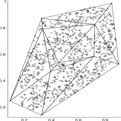
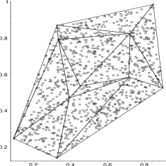
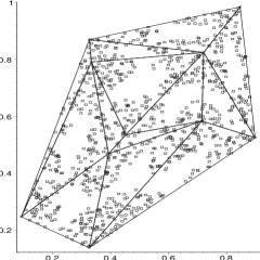
Figure 11: Realization of segregation (left), $H_{o}:CSR$ (middle), and association (right) for $|\mathcal{Y}_{m}|=10$.

For $J_{m}>1$ (i.e., $m>3$), as in Section 2, let $\widetilde{\rho}_{{}_{PE}}(n,m,r)=\left|\mathcal{A}\right|/(n\,(n-1))$ be the relative density for the proportional-edge PCD in the multiple triangle case. Let $\widetilde{\rho}_{{}_{CS}}(n,m,\tau)$ and $\rho^{{}^{[i]}}_{{}_{CS}}(\tau)$ be defined similarly for the central similarity PCD. Let $n_{i}$ be the number of $\mathcal{X}$ points in $T_{i}$ for $i=1,2,\ldots,J_{m}$. Letting $w_{i}=A(T_{i})/A(C_{H}(\mathcal{Y}_{m}))$ with $A(\cdot)$ being the area function and $\mathcal{W}=\{w_{1},w_{2},\ldots,w_{J_{m}}\}$, we obtain the following as a corollary to Theorems 3.3 and 3.4.

Corollary 3.5.

For $r\in[1,\infty]$, the asymptotic distribution for $\widetilde{\rho}_{{}_{PE}}(n,m,r)$ conditional on $\mathcal{W}$ is given by

$$\sqrt{n}\left(\widetilde{\rho}_{{}_{PE}}(n,m,r)-\widetilde{\mu}_{{}_{PE}}(m,r)\right)\stackrel{{\scriptstyle\mathcal{L}}}{{\longrightarrow}}\\ \mathcal{N}\left(0,4\,\widetilde{\nu}_{{}_{PE}}(m,r)\right),$$ (14)

as $n\rightarrow\infty$, where $\widetilde{\mu}_{{}_{PE}}(m,r)=\mu_{{}_{PE}}(r)\left(\sum_{i=1}^{J_{m}}w_{i}^{2}\right)$ and

$$\widetilde{\nu}_{{}_{PE}}(m,r)=\left[\nu_{{}_{PE}}(r)\left(\sum_{i=1}^{J_{m}}w_{i}^{3}\right)+\left(\mu_{{}_{PE}}(r)\right)^{2}\left(\sum_{i=1}^{J_{m}}w_{i}^{3}-\left(\sum_{j=1}^{J_{m}}w_{i}^{2}\right)^{2}\right)\right]$$

with $\mu_{{}_{PE}}(r)$ and $\nu_{{}_{PE}}(r)$ being as in Equations (8) and (9), respectively. The asymptotic distribution of $\widetilde{\rho}_{CS}(n,m,\tau)$ with $\tau\in(0,\infty]$ is similar.

Proof: The expectation of $\widetilde{\rho}_{{}_{PE}}(n,m,r)$ is

$$\mathbf{E}\left[\widetilde{\rho}_{{}_{PE}}(n,m,r)\right]=\frac{1}{n\,(n-1)}\sum\sum_{i<j\hskip 18.06749pt}\,\mathbf{E}\left[h_{ij}(r)\right]=\mathbf{E}\left[h_{12}(r)\right]/2=P(X_{2}\in N_{PE}(X_{1},r))=\widetilde{\mu}_{{}_{PE}}(r).$$

By definition of $N_{PE}(\cdot,r)$, if $X_{1}$ and $X_{2}$ are in different triangles, then $P(X_{2}\in N_{PE}(X_{1},r))=0$. So by the law of total probability

$$\widetilde{\mu}_{{}_{PE}}(r) := P(X_{2}\in N_{PE}(X_{1},r))=\sum_{i=1}^{J_{m}}P(X_{2}\in N_{PE}(X_{1},r)\,|\,\{X_{1},X_{2}\}\subset T_{i})\,P(\{X_{1},X_{2}\}\subset T_{i})$$

$$= \sum_{i=1}^{J_{m}}\mu_{{}_{PE}}(r)\,P(\{X_{1},X_{2}\}\subset T_{i})\text{ (since $P(X_{2}\in N_{PE}(X_{1},r)\,|\,\{X_{1},X_{2}\}\subset T_{i})=\mu_{{}_{PE}}(r)$)}$$

$$= \mu_{{}_{PE}}(r)\,\sum_{i=1}^{J_{m}}\left(\frac{A(T_{i})}{\sum_{i=1}^{J_{m}}A(T_{i})}\right)^{2}\text{ (since $P(\{X_{1},X_{2}\}\subset T_{i})=\left(\frac{A(T_{i})}{\sum_{i=1}^{J_{m}}A(T_{i})}\right)^{2}$)}$$

$$= \mu_{{}_{PE}}(r)\,\left(\sum_{i=1}^{J_{m}}w_{i}^{2}\right).$$

where $\mu_{{}_{PE}}(r)$ is given by Equation (8).

Likewise, we get $\widetilde{\mu}_{{}_{CS}}(\tau)=\mu_{{}_{CS}}(\tau)\,\left(\sum_{i=1}^{J_{m}}w_{i}^{2}\right)$ where $\mu_{{}_{CS}}(\tau)$ is given by Equation (11).

Furthermore, the asymptotic variance is

$$\widetilde{\nu}_{{}_{PE}}(m,r) = \mathbf{E}[h_{12}\,h_{13}]-\mathbf{E}[h_{12}]\,\mathbf{E}[h_{13}]$$

$$= P\bigl{(}\{X_{2},X_{3}\}\subset N_{PE}(X_{1},r)\bigr{)}+2\,P\bigl{(}X_{2}\in N_{PE}(X_{1},r),X_{3}\in\Gamma^{{}^{PE}}_{1}(X_{1},r)\bigr{)}$$

$$+P\bigl{(}\{X_{2},X_{3}\}\subset\Gamma^{{}^{PE}}_{1}(X_{1},r)\bigr{)}-4\,(\widetilde{\mu}_{{}_{PE}}(m,r))^{2}.$$

Let $P_{{}_{PE}}^{2N}(r):=P\bigl{(}\{X_{2},X_{3}\}\subset N_{PE}(X_{1},r)\bigr{)}$, $P_{{}_{PE}}^{2G}(r):=P\bigl{(}\{X_{2},X_{3}\}\subset\Gamma^{{}^{PE}}_{1}(X_{1},r)\bigr{)}$, and $P_{{}_{PE}}^{M}(r):=P\bigl{(}X_{2}\in N_{PE}(X_{1},r),X_{3}\in\Gamma^{{}^{PE}}_{1}(X_{1},r)\bigr{)}$. Then for $J_{m}>1$, we have

$$P\bigl{(}\{X_{2},X_{3}\}\subset N_{PE}(X_{1},r)\bigr{)} = \sum_{j=1}^{J_{m}}P\bigl{(}\{X_{2},X_{3}\}\subset N_{PE}(X_{1},r)\,|\,\{X_{1},X_{2},X_{3}\}\subset T_{j}\bigr{)}\,P\bigl{(}\{X_{1},X_{2},X_{3}\}\subset T_{j}\bigr{)}$$

$$= \sum_{j=1}^{J_{m}}P_{{}_{PE}}^{2N}(r)\,\bigl{(}A(T_{j})/A(C_{H}(\mathcal{Y}_{m}))\bigr{)}^{3}=P_{{}_{PE}}^{2N}(r)\,\left(\sum_{j=1}^{J_{m}}w_{j}^{3}\right).$$

Similarly, $P\bigl{(}X_{2}\in N_{PE}(X_{1},r),X_{3}\in\Gamma^{{}^{PE}}_{1}(X_{1},r)\bigr{)}=P_{{}_{PE}}^{M}(r)\,\left(\sum_{j=1}^{J_{m}}w_{j}^{3}\right)\text{ and }P\bigl{(}\{X_{2},X_{3}\}\subset\Gamma^{{}^{PE}}_{1}(X_{1},r)\bigr{)}=P_{{}_{PE}}^{2G}(r)\,\left(\sum_{j=1}^{J_{m}}w_{j}^{3}\right)$, hence,

$$\widetilde{\nu}_{{}_{PE}}(m,r)=\bigl{(}P_{{}_{PE}}^{2N}(r)+2\,P^{r}_{M}+P_{{}_{PE}}^{2G}(r)\bigr{)}\,\left(\sum_{j=1}^{J_{m}}w_{j}^{3}\right)-4\,\widetilde{\mu}_{{}_{PE}}(m,r)^{2}=\nu_{{}_{PE}}(r)\,\left(\sum_{j=1}^{J_{m}}w_{j}^{3}\right)+4\,\mu_{{}_{PE}}(r)^{2}\,\left(\sum_{j=1}^{J_{m}}w_{j}^{3}-\left(\sum_{j=1}^{J_{m}}w_{j}^{2}\right)^{2}\right),$$

Likewise, we get $\widetilde{\nu}_{{}_{CS}}(\tau)=\nu_{{}_{CS}}(\tau)\,\left(\sum_{i=1}^{J_{m}}w_{i}^{3}\right)+4\,\mu_{{}_{CS}}(\tau)^{2}\,\left(\sum_{i=1}^{J_{m}}w_{i}^{3}-\left(\sum_{i=1}^{J_{m}}w_{i}^{2}\right)^{2}\right).$

So, conditional on $\mathcal{W}$, if $\widetilde{\nu}_{{}_{PE}}(r)>0$, then $\sqrt{n}\,\left(\widetilde{\rho}_{{}_{PE}}(n,m,r)-\widetilde{\mu}_{{}_{PE}}(r)\right)\stackrel{{\scriptstyle\mathcal{L}}}{{\longrightarrow}}\mathcal{N}\left(0,\widetilde{\nu}_{{}_{PE}}(r)\right)$. A similar result holds for the relative density of the central similarity PCD. $\blacksquare$

By an appropriate application of the Jensen’s inequality, we see that $\sum_{i=1}^{J_{m}}w_{i}^{3}\geq\left(\sum_{i=1}^{J_{m}}w_{i}^{2}\right)^{2}.$ So the covariance above is zero iff $\nu_{{}_{PE}}(r)=0$ and $\sum_{i=1}^{J_{m}}w_{i}^{3}=\left(\sum_{i=1}^{J_{m}}w_{i}^{2}\right)^{2}$, so asymptotic normality may hold even though $\nu_{{}_{PE}}(r)=0$ in the multiple triangle case. That is, $\widetilde{\rho}_{{}_{PE}}(n,m,r)$ has the asymptotic normality for $r=\infty$ also provided that $\sum_{i=1}^{J_{m}}w_{i}^{3}>\left(\sum_{i=1}^{J_{m}}w_{i}^{2}\right)^{2}$. The same holds for $\tau=\infty$ in the central similarity case.

4 Alternative Patterns: Segregation and Association

In a two class setting, the phenomenon known as segregation occurs when members of one class have a tendency to repel members of the other class. For instance, it may be the case that one type of plant does not grow well in the vicinity of another type of plant, and vice versa. This implies, in our notation, that $X_{i}$ are unlikely to be located near elements of $\mathcal{Y}_{m}$. Alternatively, association occurs when members of one class have a tendency to attract members of the other class, as in symbiotic species, so that $X_{i}$ will tend to cluster around the elements of $\mathcal{Y}_{m}$, for example. See, for instance, Dixon, (1994) and Coomes et al., (1999).

These alternatives can be parametrized as follows. In the one triangle case, without loss of generality let $\mathcal{Y}_{3}=\left\{(0,0),(1,0),(c_{1},c_{2})\right\}$ and $T_{b}=T(\mathcal{Y}_{3})$ with $\mathsf{y}_{1}=(0,0),\mathsf{y}_{2}=(1,0)$, and $\mathsf{y}_{3}=(c_{1},c_{2})$. For the basic triangle $T_{b}$, let $Q_{\theta}:=\{x\in T_{b}:d(x,\mathcal{Y}_{3})\leq\theta\}$ for $\theta\in(0,(c_{1}^{2}+c_{2}^{2})/2]$ and $S(F)$ be the support of $F$. Then consider

$$\mathscr{H}_{S}:=\{F:S(F)\subseteq T_{b}\text{ and }P_{F}(X\in Q_{\theta})<P_{U}(X\in Q_{\theta})\}$$

and

$$\mathscr{H}_{A}:=\{F:S(F)\subseteq T_{b}\text{ and }P_{F}(X\in Q_{\theta})>P_{U}(X\in Q_{\theta})\}$$

where $P_{F}$ and $P_{U}$ are probabilities with respect to distribution function $F$ and the uniform distribution on $T_{b}$, respectively. So if $X_{i}\stackrel{{\scriptstyle iid}}{{\sim}}F\in\mathscr{H}_{S}$, the pattern between class $\mathcal{X}$ and $\mathcal{Y}$ points is segregation, but if $X_{i}\stackrel{{\scriptstyle iid}}{{\sim}}F\in\mathscr{H}_{A}$, the pattern between class $\mathcal{X}$ and $\mathcal{Y}$ points is association. For example the distribution family

$$\mathscr{F}_{S}:=\{F:S(F)\subset T_{b}\text{ and the associated pdf $f$ increases as $d(x,\mathcal{Y}_{3})$ increases}\}$$

is a subset of $\mathscr{H}_{S}$ and yields samples from the segregation alternatives. Likewise, the distribution family

$$\mathscr{F}_{A}:=\{F:S(F)\subset T_{b}\text{ and the associated pdf $f$ increases as $d(x,\mathcal{Y}_{3})$ decreases}\}$$

is a subset of $\mathscr{H}_{A}$ and yields samples from the association alternatives.

In the basic triangle, $T_{b}$, we define the alternatives $H^{S}_{\varepsilon}$ and $H^{A}_{\varepsilon}$ with $\varepsilon\in\left(0,\sqrt{3}/3\right)$, for segregation and association alternatives, respectively. Under $H^{S}_{\varepsilon}$, $4\varepsilon^{2}/3\times 100$ % of the area of $T_{b}$ is chopped off around each vertex so that the $\mathcal{X}$ points are restricted to lie in the remaining region. That is, for $\mathsf{y}_{j}\in\mathcal{Y}_{3}$, let $e_{j}$ denote the edge of $T_{b}$ opposite vertex $\mathsf{y}_{j}$ for $j=1,2,3$, and for $x\in T_{b}$, let $\ell_{j}(x)$ denote the line parallel to $e_{j}$ through $x$. Then define $T_{j}(\varepsilon)=\{x\in T_{b}:d(\mathsf{y}_{j},\ell_{j}(x))\leq\varepsilon_{j}\}$ where $\displaystyle\varepsilon_{1}=\frac{2\,c_{2}\,\varepsilon}{3\sqrt{c_{2}^{2}+(1-c_{1})^{2}}}$, $\displaystyle\varepsilon_{2}=\frac{2\,c_{2}\,\varepsilon}{3\sqrt{c_{1}^{2}+c_{2}^{2}}}$, and $\displaystyle\varepsilon_{3}=\frac{2\,c_{2}\,\varepsilon}{3}$. Let $\mathcal{T}_{\varepsilon}:=\bigcup_{j=1}^{3}T_{j}(\varepsilon)$. Then under $H^{S}_{\varepsilon}$, we have $X_{i}\stackrel{{\scriptstyle iid}}{{\sim}}\mathcal{U}\left(T_{b}\setminus\mathcal{T}_{\varepsilon}\right)$. Similarly, under $H^{A}_{\varepsilon}$, we have $X_{i}\stackrel{{\scriptstyle iid}}{{\sim}}\mathcal{U}\left(\mathcal{T}_{\sqrt{3}/3-\varepsilon}\right)$. Thus the segregation model excludes the possibility of any $X_{i}$ occurring around a $\mathsf{y}_{j}$, and the association model requires that all $X_{i}$ occur around $\mathsf{y}_{j}$’s. The $\sqrt{3}/3-\varepsilon$ is used in the definition of the association alternative so that $\varepsilon=0$ yields $H_{o}$ under both classes of alternatives. Thus, we have the below parametrization of the distribution families under the alternatives.

$$\mathscr{U}^{S}_{\varepsilon}:=\{F:F=\mathcal{U}(T_{b}\setminus\mathcal{T}_{\varepsilon})\}\text{ ~{}and~{} }\mathscr{U}^{A}_{\varepsilon}:=\{F:F=\mathcal{U}(\mathcal{T}_{\sqrt{3}/3-\varepsilon})\}.$$ (15)

Clearly $\mathscr{U}^{S}_{\varepsilon}\subsetneq\mathscr{H}_{S}$ and $\mathscr{U}_{\sqrt{3}/3-\varepsilon}^{A}\subsetneq\mathscr{H}_{A}$, but $\mathscr{U}^{S}_{\varepsilon}\nsubseteq\mathscr{F}_{S}$ and $\mathscr{U}_{\sqrt{3}/3-\varepsilon}^{A}\nsubseteq\mathscr{F}_{A}$.

These alternatives $H^{S}_{\varepsilon}$ and $H^{A}_{\varepsilon}$ with $\varepsilon\in\left(0,\sqrt{3}/3\right)$, can be transformed into the equilateral triangle as in Ceyhan et al., (2006) and Ceyhan et al., (2007).

For the standard equilateral triangle, in $T_{j}(\varepsilon)=\{x\in T_{e}:d(\mathsf{y},\ell_{j}(x))\leq\varepsilon_{j}\}$, we have $\varepsilon_{1}=\varepsilon_{2}=\varepsilon_{3}=\varepsilon$. Thus $H^{S}_{\varepsilon}$ implies $X_{i}\stackrel{{\scriptstyle iid}}{{\sim}}\mathcal{U}\left(T_{e}\setminus\mathcal{T}_{\varepsilon}\right)$ and $H^{A}_{\varepsilon}$ be the model under which $X_{i}\stackrel{{\scriptstyle iid}}{{\sim}}\mathcal{U}\left(\mathcal{T}_{\sqrt{3}/3-\varepsilon}\right)$. See Figure 12 for a depiction of the above segregation and the association alternatives in $T_{e}$.

Figure 12: An example for the segregation alternative with a particular expansion parameter $\varepsilon$ (shaded region), and its complement is for the association alternative with expansion parameter $\sqrt{3}/3-\varepsilon$ (unshaded region) on the standard equilateral triangle.

Remark 4.1.

The geometry invariance result of Theorem 3.1 also holds under the alternatives $H^{S}_{\varepsilon}$ and $H^{A}_{\varepsilon}$ for both PCD families. In particular, the segregation alternative with $\varepsilon\in\left(0,\sqrt{3}/4\right)$ in the standard equilateral triangle corresponds to the case that in an arbitrary triangle, $\kappa\times 100\%$ of the area is carved away as forbidden from the vertices using line segments parallel to the opposite edge where $\kappa=4\varepsilon^{2}$ (which implies $\kappa\in(0,3/4)$). But the segregation alternative with $\varepsilon\in\left(\sqrt{3}/4,\sqrt{3}/3\right)$ in the standard equilateral triangle corresponds to the case that in an arbitrary triangle, $\kappa\times 100\%$ of the area is carved away as forbidden from each vertex using line segments parallel to the opposite edge where $\kappa=1-4\left(1-\sqrt{3}\varepsilon\right)^{2}$ (which implies $\kappa\in(3/4,1)$). This argument is for the segregation alternative; a similar construction is available for the association alternative. $\square$

Remark 4.2.

The Alternatives in the Multiple Triangle Case: In the multiple triangle case, the segregation and association alternatives, $H^{S}_{\varepsilon}$ and $H^{A}_{\varepsilon}$ with $\varepsilon\in\left(0,\sqrt{3}/3\right)$, are defined as in the one-triangle case, in the sense that, when each triangle (together with the data in it) is transformed to the standard equilateral triangle as in Theorem 3.1, we obtain the same alternative pattern described above.

Thus in the case of $J_{m}>1$, we have a (conditional) test of $H_{o}:X_{i}\stackrel{{\scriptstyle iid}}{{\sim}}\mathcal{U}(C_{H}(\mathcal{Y}_{m}))$ which once again rejects against segregation for large values of $\rho_{n}(\tau,J)$ and rejects against association for small values of $\rho_{n}(\tau,J)$. The segregation (with $\kappa=1/16$, i.e., $\varepsilon=\sqrt{3}/8$), null, and association (with $\kappa=1/4$, i.e., $\varepsilon=\sqrt{3}/12$) realizations (from left to right) are depicted in Figure 11 with $n=1000$. $\square$

4.1 Asymptotic Normality under the Alternatives

Asymptotic normality of relative density of the PCDs under both alternative hypotheses of segregation and association can be established by the same method as under the null hypothesis. Let $\mathbf{E}^{S}_{\varepsilon}[\cdot]$ ($\mathbf{E}^{A}_{\varepsilon}[\cdot]$) be the expectation with respect to the uniform distribution under the segregation ( association ) alternatives with $\varepsilon\in\left(0,\sqrt{3}/3\right)$.

Theorem 4.3.

• Let $\mu^{S}_{{}_{PE}}(r,\varepsilon)$ be the mean $\mathbf{E}^{S}_{\varepsilon}[h_{12}]$ and $\nu^{S}_{{}_{PE}}(r,\varepsilon)$ be the covariance, $\mathbf{Cov}^{S}_{\varepsilon}[h_{12},h_{13}]$ for $r\in[1,\infty]$ and $\varepsilon\in\bigl{[}0,\sqrt{3}/3\bigr{)}$ under $H^{S}_{\varepsilon}$. Then as $n\rightarrow\infty$, $\sqrt{n}\bigl{(}\rho_{{}_{PE}}(n,r)-\mu^{S}_{{}_{PE}}(r,\varepsilon)\bigr{)}\stackrel{{\scriptstyle\mathcal{L}}}{{\longrightarrow}}\mathcal{N}(0,\nu^{S}_{{}_{PE}}(r,\varepsilon))$ for the values of $(r,\varepsilon)$ for which $\nu^{S}_{{}_{PE}}(r,\varepsilon)>0$. A similar result holds under association.

• Let $\mu^{S}_{{}_{CS}}(\tau,\varepsilon)$ be the mean $\mathbf{E}^{S}_{\varepsilon}[h_{12}]$ and $\nu^{S}_{{}_{CS}}(\tau,\varepsilon)$ be the covariance, $\mathbf{Cov}^{S}_{\varepsilon}[h_{12},h_{13}]$ for $\tau\in(0,\infty]$ and $\varepsilon\in\bigl{[}0,\sqrt{3}/3\bigr{)}$ under $H^{S}_{\varepsilon}$. Then as $n\rightarrow\infty$, $\sqrt{n}\bigl{(}\rho_{{}_{CS}}(n,\tau)-\mu^{S}_{{}_{PE}}(\tau,\varepsilon)\bigr{)}\stackrel{{\scriptstyle\mathcal{L}}}{{\longrightarrow}}\mathcal{N}(0,\nu^{S}_{{}_{CS}}(\tau,\varepsilon))$ for the values of $(\tau,\varepsilon)$ for which $\nu^{S}_{{}_{PE}}(\tau,\varepsilon)>0$. A similar result holds under association.

A sketch of the proof of part (i) is provided in (Ceyhan et al., (2006)), and of part (ii) for $\tau\in(0,1]$ is provided in (Ceyhan et al., (2007)). The proof of part (ii) for $\tau\in(1,\infty)$ is similar.

The explicit forms of $\mu^{S}_{{}_{PE}}(r,\varepsilon)$ and $\mu^{A}_{{}_{PE}}(r,\varepsilon)$ are given, defined piecewise, in (Ceyhan et al., 2004b ). Note that under $H^{S}_{\varepsilon}$,

$$\nu^{S}_{{}_{PE}}(r,\varepsilon)>0\text{ for }(r,\varepsilon)\in\left[1,\sqrt{3}/(2\varepsilon)\right)\times\left(0,\sqrt{3}/4\right]\bigcup\left[1,\sqrt{3}/\varepsilon-2\right)\times\left(\sqrt{3}/4,\sqrt{3}/3\right),$$

and under $H^{A}_{\varepsilon}$,

$$\nu^{A}_{{}_{PE}}(r,\varepsilon)>0\text{ for }(r,\varepsilon)\in(1,\infty)\times\left(0,\sqrt{3}/3\right)\bigcup\{1\}\times\left(0,\sqrt{3}/12\right).$$

The explicit forms of $\mu^{S}_{{}_{CS}}(\tau,\varepsilon)$ and $\mu^{A}_{{}_{CS}}(\tau,\varepsilon)$ are given, defined piecewise, in (Ceyhan et al., 2004a ). Note that under $H^{S}_{\varepsilon}$,

$$\nu^{S}_{{}_{CS}}(\tau,\varepsilon)>0\text{ for }(\tau,\varepsilon)\in(0,\infty)\times\bigl{(}0,3\,\sqrt{3}/10\Bigr{]}\bigcup\Biggl{(}\frac{2\,(\sqrt{3}-3\,\varepsilon)}{4\,\varepsilon-\sqrt{3}},\infty\Biggr{]}\times\bigl{(}3\,\sqrt{3}/10,\sqrt{3}/3\bigr{)},$$

and under $H^{A}_{\varepsilon}$,

$$\nu^{A}_{{}_{CS}}(\tau,\varepsilon)>0\text{ for }(\tau,\varepsilon)\in(0,\infty]\times\bigl{(}0,\sqrt{3}/3\bigr{)}.$$

Notice that under association alternatives any $r\in[1,\infty)$ yields asymptotic normality for relative density of proportional-edge PCD for all $\varepsilon\in\left(0,\sqrt{3}/3\right)$, while under segregation alternatives, only $r=1$ yields this universal asymptotic normality. Furthermore, under association alternatives any $\tau\in(0,\infty)$ yields asymptotic normality for relative density of central similarity PCD for all $\varepsilon\in\bigl{(}0,\sqrt{3}/3\bigr{)}$. The same holds under segregation alternatives.

The asymptotic normality also holds under the alternatives in the multiple triangle case. For example, for the relative density of proportional-edge PCDs, the asymptotic mean and variance are as in Corollary 3.5 with $\mu_{{}_{PE}}(r)$ ($\nu_{{}_{PE}}(r)$) being replaced by $\mu^{S}_{{}_{PE}}(r,\varepsilon)$ ($\nu^{S}_{{}_{PE}}(r,\varepsilon)$) for segregation and by $\mu^{A}_{{}_{PE}}(r,\varepsilon)$ ($\nu^{A}_{{}_{PE}}(r,\varepsilon)$) for association.

and

4.2 The Test Statistics and Analysis

The relative density of the PCD is a test statistic for the segregation/association alternative; rejecting for extreme values of $\rho_{{}_{PE}}(n,r)$ is appropriate since under segregation we expect $\rho_{{}_{PE}}(n,r)$ to be large, while under association we expect $\rho_{{}_{PE}}(n,r)$ to be small.

In the one triangle case, using the standardized test statistic

$$R_{PE}(r)=\frac{\sqrt{n}\bigl{(}\rho_{{}_{PE}}(n,r)-\mu_{{}_{PE}}(r)\bigr{)}}{\sqrt{\nu_{{}_{PE}}(r)}},$$ (16)

the asymptotic critical value for the one-sided level $\alpha$ test against segregation is given by

$$z_{\alpha}=\Phi^{-1}(1-\alpha)$$ (17)

where $\Phi(\cdot)$ is the standard normal distribution function. Against segregation, the test rejects for $R_{PE}(r)>z_{\alpha}$ and against association, the test rejects for $R_{PE}(r)<z_{1-\alpha}$. The same holds for the standardized test statistic in the multiple triangle case, $\widetilde{R}_{PE}(r)=\frac{\sqrt{n}\bigl{(}\widetilde{\rho}_{{}_{PE}}(n,r)-\widetilde{\mu}_{{}_{PE}}(r)\bigr{)}}{\sqrt{\widetilde{\nu}_{{}_{PE}}(r)}}$.

A similar construction is available for $\rho_{{}_{CS}}(n,\tau)$ with

$$R_{CS}(\tau)=\frac{\sqrt{n}\bigl{(}\rho_{{}_{CS}}(n,\tau)-\mu_{{}_{CS}}(\tau)\bigr{)}}{\sqrt{\nu_{{}_{CS}}(\tau)}}$$ (18)

in the one triangle case, and with $\widetilde{R}_{CS}(\tau)=\frac{\sqrt{n}\bigl{(}\widetilde{\rho}_{{}_{CS}}(n,\tau)-\widetilde{\mu}_{{}_{CS}}(\tau)\bigr{)}}{\sqrt{\widetilde{\nu}_{{}_{CS}}(\tau)}}$ in the multiple triangle case.

4.3 Consistency

Theorem 4.4.

• In the one triangle case, the test against $H^{S}_{\varepsilon}$ which rejects for $R_{PE}(r)>z_{1-\alpha}$ and the test against $H^{A}_{\varepsilon}$ which rejects for $R_{PE}(r)<z_{\alpha}$ are consistent for $r\in[1,\infty)$ and $\varepsilon\in\left(0,\sqrt{3}/3\right)$. The same holds in the multiple triangle case with $\widetilde{R}_{PE}(r)$.

• In the one triangle case, the test against $H^{S}_{\varepsilon}$ which rejects for $R_{CS}(\tau)>z_{1-\alpha}$ and the test against $H^{A}_{\varepsilon}$ which rejects for $R_{CS}(\tau)<z_{\alpha}$ are consistent for $\tau\in(0,\infty)$ and $\varepsilon\in\left(0,\sqrt{3}/3\right)$. The same holds in the multiple triangle case with $\widetilde{R}_{CS}(\tau)$.

For the one triangle case, the proof of (i) is provided in (Ceyhan et al., (2006)) and the proof of (ii) with $\tau\in(0,1]$ is provided in (Ceyhan et al., (2007)). The proofs for the multiple triangle cases and for (ii) with $\tau>1$ are similar.

5 Empirical Size Analysis

5.1 Empirical Size Analysis for Proportional-Edge PCDs under CSR

In one triangle case, for the null pattern of CSR, we generate $n$ $\mathcal{X}$ points iid $\mathcal{U}(T_{e})$ where $T_{e}$ is the standard equilateral triangle. We calculate the relative density of proportional-edge PCDs for $r=1,11/10,6/5,4/3,\sqrt{2},\\ 3/2,2,3,5,10$ at each Monte Carlo replicate. We repeat the Monte Carlo procedure $N_{mc}=10000$ times for each of $n=10,50,100$. Using the critical values based on the normal approximation for the relative density, we calculate the empirical size estimates for both right-sided (i.e., for segregation) and left-sided (i.e., for association) tests as a function of the expansion parameter $r$. Let $R_{PE}(r)(r,j):=\frac{\sqrt{n}\,\bigl{(}\rho_{{}_{PE}}(n,r,j)-\mu_{{}_{PE}}(r)\bigr{)}}{\sqrt{\nu_{{}_{PE}}(r)}}$ be the standardized relative density for Monte Carlo replicate $j$ with sample size $n$ for $j=1,2,\ldots,N_{mc}$. For each $r$ value, the level $\alpha$ asymptotic critical value is $\mu_{{}_{PE}}(r)+z_{(1-\alpha)}\cdot\sqrt{\nu_{{}_{PE}}(r)/n}$. We estimate the empirical size against the segregation alternative as $\frac{1}{N_{mc}}\sum_{j=1}^{N_{mc}}\mathbf{I}\left(R_{PE}(r)(r,j)>z_{1-\alpha}\right)$, and against the association alternative as $\frac{1}{N_{mc}}\sum_{j=1}^{N_{mc}}\mathbf{I}\left(R_{PE}(r)(r,j)<z_{\alpha}\right)$. The empirical sizes significantly smaller (larger) than .05 are deemed conservative (liberal). The asymptotic normal approximation to proportions is used in determining the significance of the deviations of the empirical sizes from .05. For these proportion tests, we also use $\alpha=.05$ as the significance level. With $N_{mc}=10000$, empirical sizes less than .0464 are deemed conservative, greater than .0536 are deemed liberal at $\alpha=.05$ level. The empirical sizes for the proportional-edge PCDs together with upper and lower limits of liberalness and conservativeness are plotted in Figure 13. Observe that as $n$ increases, the empirical size gets closer to the nominal level of 0.05 (i.e., the normal approximation gets better). For the right-sided tests (i.e., relative to segregation) the size is close to the nominal level for $r\in(2,3)$, for smaller $r$ values (i.e., $r<2$) the test seems to be liberal with liberalness increasing as $r$ decreases; and for larger $r$ values (i.e., $r>3$) the test seems to be conservative with conservativeness increasing as $r$ increases. For the left-sided tests (i.e., relative to association) the size is close to the nominal level for $r\in(1.5,3)$, for other $r$ values the test seems to be liberal (more liberal for smaller $r$ values). This is due to the fact that very large and small values of $r$ require much larger sample sizes for the normal approximation to hold.

Figure 13: Empirical size for $R_{PE}(r)$ in the one triangle case: The empirical size estimates of the relative density of proportional-edge PCDs in the one triangle case based on 10000 Monte Carlo replicates for the left-sided alternative, i.e., relative to segregation (top) and the right-sided alternative, i.e., relative to association (bottom) with $n=10$ (left column), $n=50$ (middle column), and $n=100$ (right column) under the CSR pattern. The horizontal lines are located at .0464 (upper threshold for conservativeness), .050 (nominal level), and .0536 (lower threshold for liberalness).

In the multiple triangle case, for the null pattern of CSR, we generate $n$ $\mathcal{X}$ points iid $\mathcal{U}(C_{H}(\mathcal{Y}_{10}))$ where $\mathcal{Y}_{10}$ is the set of the 10 class $\mathcal{Y}$ points given in Figure 11. With $N_{mc}=1000$, empirical sizes less than .039 are deemed conservative, greater than .061 are deemed liberal at $\alpha=.05$ level. The empirical sizes for the proportional-edge PCDs together with upper and lower limits of liberalness and conservativeness are plotted in Figure 14. Observe that in the multiple triangle case (which is more realistic than the one triangle case) the empirical sizes are much closer to the nominal level compared to the one triangle case. For the right-sided alternative (i.e., against segregation), the size is about the nominal level for $r\in(1.5,3)$, and for the left-sided alternative (i.e., against association), the size is about the nominal level for $r\in(1.1,2)$. Furthermore, although the empirical sizes for both right- and left-sided alternatives are about the desired level for $r$ values between 1.5 and 2, it seems that they are not very far from the nominal level for $r\in(1.5,10)$. The test seems to be liberal for the right-sided alternative and conservative for the left-sided alternative, if not at the desired level.

Figure 14: Empirical size for $R_{PE}(r)$ in the multiple triangle case: The empirical size estimates of the relative density of proportional-edge PCDs in the multiple triangle case based on 1000 Monte Carlo replicates for the right-sided alternative (i.e., relative to segregation) (top) and the left-sided alternative (i.e., relative to association) (bottom) with $n=500$ (left column) and $n=1000$ (right column) under the CSR pattern. The horizontal lines are located at .039 (upper threshold for conservativeness), .050 (nominal level), and .061 (lower threshold for liberalness).

5.2 Empirical Size Analysis for Central Similarity PCDs under CSR

In one and multiple triangle cases, data generation is as in Section 5.1 and we compute the relative density of central similarity PCDs for $\tau=0.2,0.4,0.6.\ldots,3.0,3.5,4.0,\ldots,20.0$ at each Monte Carlo replicate. Let $R_{CS}(\tau)(\tau,j):=\frac{\sqrt{n}\,\bigl{(}\rho_{CS}(n,\tau,j)-\mu_{{}_{CS}}(\tau)\bigr{)}}{\sqrt{\nu_{{}_{CS}}(\tau)}}$ be the standardized relative density for Monte Carlo replicate $j$ with sample size $n$ for $j=1,2,\ldots,N_{mc}$. For each $\tau$ value, the level $\alpha$ asymptotic critical value is $\mu_{{}_{CS}}(\tau)+z_{(1-\alpha)}\cdot\sqrt{\nu_{{}_{CS}}(\tau)/n}$. We estimate the empirical size against the segregation alternative as $\frac{1}{N_{mc}}\sum_{j=1}^{N_{mc}}\mathbf{I}\left(R_{CS}(\tau)(\tau,j)>z_{1-\alpha}\right)$ and against the association alternative as $\frac{1}{N_{mc}}\sum_{j=1}^{N_{mc}}\mathbf{I}\left(R_{CS}(\tau)(\tau,j)<z_{\alpha}\right)$. In one triangle case, the empirical sizes for the central similarity PCDs together with upper and lower limits of liberalness and conservativeness are plotted in Figure 15. Observe that as $n$ increases, the empirical size gets closer to the nominal level of 0.05 (i.e., the normal approximation gets better). For the right-sided tests, the size is close to the nominal level for $\tau\in(5,14)$ and closest to 0.05 for $\tau\approx 5$ or $\tau\in(7,9)$ for all sample sizes; for smaller $\tau$ values (i.e., $\tau\lesssim 4.5$) the test seems to be liberal with liberalness increasing as $\tau$ decreases; and for $\tau\gtrsim 15$ the test is extremely conservative with size being virtually 0 for $n=10$ and the test is slightly conservative for $n=50$ and 100. For larger $n$ (i.e., $n\geq 50$), the test has the desired size for $\tau\geq 4$. Considering all sample sizes, we recommend $\tau\in(5,10)$ for testing against segregation. For the left-sided tests with $n=10$ the size is close to the nominal level for $\tau\in(2,4)$. For $n=50$ the test has the desired size for $\tau\in(2,10)$ and for $n=100$ the test has the desired size for $\tau\in(2,15)$. With all sample sizes, the test seems to be conservative (slightly liberal) for smaller (larger) $\tau$ values. Considering all sample sizes, we recommend $\tau\in(2.5,5)$ for testing against association. The range of appropriate $\tau$ values gets wider with the increasing sample size and very large and small values of $\tau$ require much larger sample sizes for the normal approximation to hold.

Figure 15: Empirical size for $R_{CS}(\tau)$ in the one triangle case: The empirical size estimates of the relative density of central similarity PCDs in the one triangle case based on 10000 Monte Carlo replicates for the left-sided alternative (i.e., relative to segregation) (top) and the right-sided alternative (i.e., relative to association) (bottom) with $n=10$ (left column), $n=50$ (middle column), and $n=100$ (right column) under the CSR pattern. The horizontal lines are as in Figure 13.

In the multiple triangle case, the empirical sizes for the central similarity PCDs are plotted in Figure 16. Observe that in the multiple triangle case the empirical sizes are much closer to the nominal level compared to the one triangle case. Furthermore, for the right-sided alternative with $n=500$, the test has the desired level for $\tau\in(.8,4)$, $\tau\approx 5$, and $\tau\in(12,20)$ and with $n=1000$ for $\tau\geq 2$. Considering all sample sizes, we recommend $\tau\in(2.5,8)$ for testing against segregation. For the left-sided alternative, with $n=500$, $\tau\geq.5$ (except $\tau=7$ or 11) seems to yield the appropriate level and with $n=1000$, $\tau\geq.5$ seems to yield the appropriate level. Considering all sample sizes, we recommend $\tau\in(0.5,20)$ for testing against association.

Figure 16: Empirical size for $R_{CS}(\tau)$ in the multiple triangle case: The empirical size estimates of the relative density of central similarity PCDs in the multiple triangle case based on 1000 Monte Carlo replicates for the left-sided alternative (i.e., relative to segregation) (top) and the right-sided alternative (i.e., relative to association) (bottom) with $n=500$ (left column) and $n=1000$ (right column) under the CSR pattern. The horizontal lines are as in Figure 14.

Remark 5.1.

Empirical Size Comparison for the Two PCD Families: In the one triangle case, the size estimates for the central similarity PCD is close to the nominal level of 0.05 against the segregation alternative for more of the expansion parameter values considered. On the other hand, the size estimates against association are close to the nominal level for both PCD families, but it seems that the size estimates for central similarity PCD is closer to the nominal level. In the multiple triangle case, the size performance of the two PCD families is similar and the size estimates are close to the nominal level for both of the alternatives. $\square$

6 Empirical Power Analysis under the Alternatives

To compare the power performance of the test statistics under the alternatives, we generate $n$ $\mathcal{X}$ points uniformly in the corresponding support sets as described in Section 4 and provide the empirical power estimates of the tests under the segregation and association alternatives.

6.1 Empirical Power Analysis for Proportional-Edge PCDs under the Segregation Alternative

In the one triangle case, at each Monte Carlo replicate under segregation $H^{S}_{\varepsilon}$, we generate $X_{i}\stackrel{{\scriptstyle iid}}{{\sim}}\mathcal{U}\left(T_{e}\setminus\mathcal{T}_{\varepsilon}\right)$, for $i=1,2,\ldots,n$ for $n=10,50,100$. At each Monte Carlo replicate, we compute the relative density of the proportional-edge PCDs. We consider $r\in\{1,11/10,6/5,4/3,\sqrt{2},3/2,2,3,5,10\}$ for the proportional-edge PCD. We repeat the above simulation procedure $N_{mc}=10000$ times. We consider $\varepsilon\in\{\sqrt{3}/8,\sqrt{3}/4,2\,\sqrt{3}/7\}$ (which correspond to 18.75 %, 75 %, and $4500/49\approx 91.84$ % of the triangle (around the vertices) being unoccupied by the $\mathcal{X}$ points, respectively) for the segregation alternatives.

Under segregation alternatives with $\varepsilon>0$, the distribution of $\rho_{{}_{PE}}(n,r)$ is degenerate for large values of $r$. For a given $\varepsilon\in(0,\sqrt{3}/4)$, the corresponding digraph is complete almost surely, for $r\geq\frac{\sqrt{3}}{2\varepsilon}$, hence $\rho_{{}_{PE}}(n,r)=1$ a.s. For $\varepsilon\in(\sqrt{3}/4,\sqrt{3}/3)$, the corresponding digraph is complete almost surely, for $r\geq\frac{\sqrt{3}-2\varepsilon}{\varepsilon}$. In particular, for $\varepsilon=\sqrt{3}/8$, $\rho_{{}_{PE}}(n,r)$ is degenerate for $r\geq 4$, for $\varepsilon=\sqrt{3}/4$, $\rho_{{}_{PE}}(n,r)$ is degenerate for $r\geq 2$, and for $\varepsilon=2\,\sqrt{3}/7$, $\rho_{{}_{PE}}(n,r)$ is degenerate for $r\geq 3/2$,

\psfrag{kernel density estimate}{ \Huge{{kernel density estimate}}}\psfrag{relative density}{ \Huge{{relative density}}}\includegraphics{segsim6.ps}

\psfrag{kernel density estimate}{ \Huge{{kernel density estimate}}}\psfrag{relative density}{ \Huge{{relative density}}}\includegraphics{seg2sim6.ps}

Figure 17: Kernel density estimates of the relative density of proportional-edge PCD, $\rho_{{}_{PE}}(n,r)$, under the null (solid line) and the segregation alternatives (dashed line) with $H^{S}_{\sqrt{3}/8}$ (left) and $H^{S}_{\sqrt{3}/4}$ (right) for $r=3/2$ with $n=10$ based on $N_{mc}=10000$ replicates.

In the one triangle case, we plot the kernel density estimates for the null case and the segregation alternative with $\varepsilon=\sqrt{3}/8$ and $\varepsilon=\sqrt{3}/4$ with $n=10$ and $N_{mc}=10000$ in Figure 17. Observe that under both $H_{o}$ and alternatives, kernel density estimates are almost symmetric for $r=3/2$. Moreover, there is much more separation between the kernel density estimates of the null and alternatives for $\varepsilon=\sqrt{3}/4$ compared to $\varepsilon=\sqrt{3}/8$, implying more power for larger $\varepsilon$ values. In Figure 18, we present a Monte Carlo investigation against the segregation alternative $H^{S}_{\sqrt{3}/8}$ for $r=11/10$, and $n=10$, $N_{mc}=10000$ (left), $n=100$, $N_{mc}=1000$ (right). With $n=10$, the null and alternative kernel density functions for $\rho_{10}(11/10)$ are very similar, implying small power. With $n=100$, there is more separation between null and alternative kernel density functions implying higher power. Notice also that the probability density functions are more skewed for $n=10$, while approximate normality holds for $n=100$.

\psfrag{kernel density estimate}{ \Huge{{kernel density estimate}}}\psfrag{relative density}{ \Huge{{relative density}}}\includegraphics{segsim2.ps}

\psfrag{kernel density estimate}{ \Huge{{kernel density estimate}}}\psfrag{relative density}{ \Huge{{relative density}}}\includegraphics{segn100sim2.ps}

Figure 18: Depicted are kernel density estimates for $\rho_{{}_{PE}}(n,11/10)$ for $n=10$ (left) and $n=100$ (right) under the null (solid line) and segregation alternative $H^{S}_{\sqrt{3}/8}$ (dashed line).

Figure 19: Empirical power for $R_{PE}(r)$ in the one triangle case: Monte Carlo power estimates for relative density of proportional-edge PCDs in the one triangle case using the asymptotic critical value against segregation alternatives $H^{S}_{\sqrt{3}/8}$ (top row), $H^{S}_{\sqrt{3}/4}$ (middle row), and $H^{S}_{2\,\sqrt{3}/7}$ (bottom row) as a function of $r$, for $n=10$ (left column), $n=50$ (middle column), and $n=100$ (right column).

For a given alternative and sample size, we analyze the empirical power of the test based on $\rho_{{}_{PE}}(n,r)$ — using the asymptotic critical value— as a function of the expansion parameter $r$. We estimate the empirical power as $\frac{1}{N_{mc}}\sum_{j=1}^{N_{mc}}\mathbf{I}\left(R_{PE}(r)(r,j)>z_{1-\alpha}\right)$. In Figure 19, we present Monte Carlo power estimates for relative density of proportional-edge PCDs in the one triangle case against $H^{S}_{\sqrt{3}/8}$, $H^{S}_{\sqrt{3}/4}$, and $H^{S}_{2\,\sqrt{3}/7}$ as a function of $r$ for $n=10,50,100$. Notice that Monte Carlo power estimate increases as $r$ gets larger and then decreases, due to the magnitude of $r$ and $n$. Because for small $n$ and large $r$, the critical value is approximately 1 under $H_{o}$, as we get a complete digraph with high probability. Moreover, the more severe the segregation, the higher the power estimate at each $r$. Under mild segregation (with $\varepsilon=\sqrt{3}/8$), $r$ around 1.5 or 5 yields the highest power (for other $r$ values, the power performance is very poor). Furthermore, under moderate to severe segregation, with $n=10$ the power estimate seems to be close to 1 for $r\in(1,4)$, and with $n=50$ or 100 the power estimate seems to be close to 1 for $r\in(1,5)$. However, the power estimates are valid only for $r$ within $(2,3)$, since the test has the desired size for this range of $r$ values against the right-sided alternative. So, for small sample sizes, $r\approx 1.5$ is recommended, and for larger sample sizes, moderate values of $r$ (i.e., $r\in(2,3)$) are recommended for the segregation alternative as they are more appropriate for normal approximation and they yield the desired significance level.

Figure 20: Empirical power for $R_{PE}(r)$ in the multiple triangle case: Monte Carlo power estimates for proportional-edge PCDs in the multiple triangle case using the asymptotic critical value against segregation alternatives $H^{S}_{\sqrt{3}/8}$ (left column), $H^{S}_{\sqrt{3}/4}$ (middle column), and $H^{S}_{2\,\sqrt{3}/7}$ (right column) as a function of $r$, for $n=500$ (top) and $n=1000$ (bottom).

In the multiple triangle case, we generate the $\mathcal{X}$ points uniformly in the support for the segregation alternatives in the triangles based on the 10 class $\mathcal{Y}$ points given in Figure 11. We use the parameters $\varepsilon\in\{\sqrt{3}/8,\sqrt{3}/4,2\,\sqrt{3}/7\}$. We compute the relative density based on the formula given in Corollary 3.5. The corresponding empirical power estimates as a function of $r$ (using the normal approximation) are presented in Figure 20 for $n=500$ or 1000. Observe that the Monte Carlo power estimate increases as $r$ gets larger and then decreases, as in the one triangle case. The empirical power is maximized for $r\in(1.5,2)$ under mild segregation, and for $r\in(1.5,3)$ under moderate to severe segregation. Considering the empirical size estimates, $r\approx 1.5$ is recommended under mild segregation, while $r\in(2,3)$ seems to be more appropriate (hence recommended for more severe segregation) since the corresponding test has the desired level with high power.

6.2 Empirical Power Analysis for Central Similarity PCDs under the Segregation Alternative

In the one triangle case, data generation is as in Section 6.1. At each Monte Carlo replicate we compute the relative density of the central similarity PCDs. We consider $\tau\in\{0.2,0.4,0.6,\ldots,3.0,3.5,4.0,\ldots,20.0\}$ for the central similarity PCD. We repeat the simulation procedure $N_{mc}=10000$ times. Under segregation alternatives with $\varepsilon>0$, the distribution of $\rho_{{}_{CS}}(n,\tau)$ is non-degenerate for all $\tau\in(0,\infty)$ and $\varepsilon\in(0,\sqrt{3}/3)$.

\psfrag{kernel density estimate}{ \Huge{{kernel density estimate}}}\psfrag{relative density}{ \Huge{{relative density}}}\includegraphics{CSsegsim10.ps}

\psfrag{kernel density estimate}{ \Huge{{kernel density estimate}}}\psfrag{relative density}{ \Huge{{relative density}}}\includegraphics{CSseg2sim10.ps}

Figure 21: Kernel density estimates of the relative density of central similarity PCD, $\rho_{{}_{CS}}(n,\tau)$, under the null (solid line) and the segregation alternatives (dashed line) with $H^{S}_{\sqrt{3}/8}$ (left) and $H^{S}_{\sqrt{3}/4}$ (right) for $\tau=1$ with $n=10$ based on $N_{mc}=10000$ replicates.

In the one triangle case, we plot the kernel density estimates for the null case and the segregation alternative with $\varepsilon=\sqrt{3}/8$ and $\varepsilon=\sqrt{3}/4$ with $n=10$ and $N_{mc}=10000$ in Figure 21. Observe that under both $H_{o}$ and alternatives, kernel density estimates are almost symmetric for $\tau=1$. Moreover, there is much more separation between the kernel density estimates of the null and alternatives for $\varepsilon=\sqrt{3}/4$ compared to $\varepsilon=\sqrt{3}/8$, implying more power for larger $\varepsilon$ values. In Figure 22, we present kernel density estimates for the null case and the segregation alternative $H^{S}_{\sqrt{3}/4}$ for $\tau=0.5$, and $n=10$, $N_{mc}=10000$ (left), $n=100$, $N_{mc}=1000$ (right). With $n=10$, the null and alternative kernel density functions for $\rho_{{}_{CS}}(10,0.5)$ are very similar, implying small power. With $n=100$, there is more separation between null and alternative kernel density functions, implying higher power. Notice also that the probability density functions are more skewed for $n=10$, while approximate normality holds for $n=100$.

\psfrag{kernel density estimate}{ \Huge{{kernel density estimate}}}\psfrag{relative density}{ \Huge{{relative density}}}\includegraphics{CSseg2sim5.ps}

\psfrag{kernel density estimate}{ \Huge{{kernel density estimate}}}\psfrag{relative density}{ \Huge{{relative density}}}\includegraphics{CSseg2sim5n100.ps}

Figure 22: Depicted are kernel density estimates for $\rho_{{}_{CS}}(n,0.5)$ for $n=10$ (left) and $n=100$ (right) under the null (solid line) and segregation alternative $H^{S}_{\sqrt{3}/4}$ (dashed line).

Figure 23: Empirical power for $R_{CS}(\tau)$ in the one triangle case: Monte Carlo power estimates for relative density of central similarity PCDs in the one triangle case using the asymptotic critical value against segregation alternatives $H^{S}_{\sqrt{3}/8}$ (top row), $H^{S}_{\sqrt{3}/4}$ (middle row), and $H^{S}_{2\,\sqrt{3}/7}$ (bottom row) as a function of $\tau$, for $n=10$ (left column), $n=50$ (middle column), and $n=100$ (right column).

We estimate the empirical power as $\frac{1}{N_{mc}}\sum_{j=1}^{N_{mc}}\mathbf{I}\left(R_{CS}(\tau)(\tau,j)>z_{1-\alpha}\right)$. In Figure 23, we present Monte Carlo power estimates for relative density of central similarity PCDs in the one triangle case against $H^{S}_{\sqrt{3}/8}$, $H^{S}_{\sqrt{3}/4}$, and $H^{S}_{2\,\sqrt{3}/7}$ as a function of $\tau$ for $n=10,50,100$. Notice that Monte Carlo power estimate increases as $\tau$ gets larger or $n$ gets larger. Moreover, the more severe the segregation, the higher the power estimate at each $\tau$. With $n=10$, the power estimates are high for $\tau\in(5,14)$ and virtually 0 for $\tau\geq 14$. With $n=50$ or $100$, the power values are high for $\tau\geq 1$, with highest power being attained around $\tau\approx 8$. However, for $\tau\geq 6$, the power values are virtually same. Considering the empirical size estimates, we recommend $\tau\approx 8$ for mild segregation, and $\tau\approx 5$ for more severe segregation alternatives.

Figure 24: Empirical power for $R_{CS}(\tau)$ in the multiple triangle case: Monte Carlo power estimates for central similarity PCDs in the multiple triangle case using the asymptotic critical value against segregation alternatives $H^{S}_{\sqrt{3}/8}$ (left column), $H^{S}_{\sqrt{3}/4}$ (middle column), and $H^{S}_{2\,\sqrt{3}/7}$ (right column) as a function of $\tau$, for $n=500$ (top) and $n=1000$ (bottom).

In the multiple triangle case, data generation is again as in Section 6.1. We compute the relative density based on the formula given in Corollary 3.5. The corresponding empirical power estimates as a function of $\tau$ (using the normal approximation) are presented in in Figure 24 for $n=500$ and $1000$. Observe that the Monte Carlo power estimate tends to increase as $\tau$ gets larger. Under mild segregation with $\varepsilon=\sqrt{3}/8$, the empirical power is large for $\tau\geq 2$ with largest being around $\tau\in(4,8)$. Under moderate to severe segregation, the empirical power is virtually one for $\tau\geq 0.4$. Considering the empirical size estimates, $\tau\approx 7$ seems to be more appropriate (hence recommended for segregation) since the corresponding test has the desired level with highest power.

6.3 Empirical Power Analysis for Proportional-Edge PCDs under the Association Alternative

In the one triangle case, at each of $N_{mc}=10000$ Monte Carlo replicates under association $H^{A}_{\varepsilon}$, we generate $X_{i}\stackrel{{\scriptstyle iid}}{{\sim}}\mathcal{U}\left(\mathcal{T}_{\sqrt{3}/3-\varepsilon}\right)$, for $i=1,2,\ldots,n$ for $n=10,50,100$. The relative density is computed as in Section 6.1. Unlike the segregation alternatives, the distribution of $\rho_{{}_{PE}}(n,r)$ is non-degenerate for all $\varepsilon\in(0,\sqrt{3}/3)$ and $r\in[1,\infty)$. We consider $\varepsilon\in\{5\,\sqrt{3}/24,\sqrt{3}/12,\sqrt{3}/21\}$ (which correspond to 18.75 %, 75 %, and $4500/49\approx 91.84$ % of the triangle being occupied around the $\mathcal{Y}$ points by the $\mathcal{X}$ points, respectively) for the association alternatives.

\psfrag{kernel density estimate}{ \Huge{{kernel density estimate}}}\psfrag{relative density}{ \Huge{{relative density}}}\includegraphics{agg3sim6.ps}

\psfrag{kernel density estimate}{ \Huge{{kernel density estimate}}}\psfrag{relative density}{ \Huge{{relative density}}}\includegraphics{aggsim6.ps}

Figure 25: Kernel density estimates of the relative density of proportional-edge PCD, $\rho_{{}_{PE}}(n,r)$, under the null (solid line) and the association alternatives (dashed line) with $H^{A}_{\sqrt{3}/21}$ (left) and $H^{A}_{5\,\sqrt{3}/24}$ (right) for $r=3/2$ with $n=10$ based on $N_{mc}=10000$ replicates.

In the one triangle case, we plot the kernel density estimates for the null case and the association alternative with $\varepsilon=\sqrt{3}/21$ and $\varepsilon=5\,\sqrt{3}/24$ with $n=10$ and $N_{mc}=10000$ in Figure 25. Observe that under both $H_{o}$ and alternatives, kernel density estimates are almost symmetric for $r=3/2$. Moreover, there is more separation between the kernel density estimates of the null and alternatives for $\varepsilon=5\,\sqrt{3}/24$ compared to $\varepsilon=\sqrt{3}/21$, implying more power for larger $\varepsilon$ values. In Figure 26, we present kernel density estimates for the null and the association alternative $H^{A}_{\sqrt{3}/12}$ for $r=11/10$, and $n=10$, $N_{mc}=10000$ (left), $n=100$, $N_{mc}=1000$ (right). With $n=10$, the null and alternative kernel density functions for $\rho_{10}(11/10)$ are very similar, implying small power. With $n=100$, there is more separation between null and alternative kernel density functions implying higher power. Notice also that the probability density functions are more skewed for $n=10$, while approximate normality holds for $n=100$.

\psfrag{kernel density estimate}{ \Huge{{kernel density estimate}}}\psfrag{relative density}{ \Huge{{relative density}}}\includegraphics{agg2sim2.ps}

\psfrag{kernel density estimate}{ \Huge{{kernel density estimate}}}\psfrag{relative density}{ \Huge{{relative density}}}\includegraphics{agg2n100sim2.ps}

Figure 26: Depicted are kernel density estimates for $\rho_{{}_{PE}}(n,11/10)$ for $n=10$ (left) and $n=100$ (right) under the null (solid line) and association alternative $H^{A}_{\sqrt{3}/12}$ (dashed line).

Figure 27: Empirical power for $R_{PE}(r)$ in the one triangle case: Monte Carlo power estimates for relative density of proportional-edge PCDs in the one triangle case using the asymptotic critical value against association alternatives $H^{A}_{\sqrt{3}/21}$ (top row), $H^{A}_{\sqrt{3}/12}$ (middle row), and $H^{A}_{5\,\sqrt{3}/24}$ (bottom row) as a function of $r$, for $n=10$ (left column), $n=50$ (middle column), and $n=100$ (right column).

Under association, for each $r$ value, the level $\alpha$ asymptotic critical value is $\mu_{{}_{PE}}(r)z_{\alpha}\cdot\sqrt{\nu_{{}_{PE}}(r)/n}$. We estimate the empirical power as $\frac{1}{N_{mc}}\sum_{j=1}^{N_{mc}}\mathbf{I}\left(R_{PE}(r)(r,j)<z_{\alpha}\right)$. In Figure 27, we present Monte Carlo power estimates for relative density of proportional-edge PCDs in the one triangle case against $H^{A}_{5\,\sqrt{3}/24}$, $H^{A}_{\sqrt{3}/12}$, and $H^{A}_{\sqrt{3}/21}$ as a function of $r$ for $n=10,50,100$. Notice that Monte Carlo power estimate increases as $r$ gets larger and then decreases, as in the segregation case. Because for small $n$ and large $r$, the critical value is approximately one under $H_{o}$, as we get a nearly complete digraph with high probability. Moreover, the more severe the association, the higher the power estimate at each $r$. Highest power is attained for $r\approx 2$, which is recommended against the association, as it yields the desired level with high power.

Figure 28: Empirical power for $R_{PE}(r)$ in the multiple triangle case: Monte Carlo power estimates of the relative density of proportional-edge PCDs in the multiple triangle case using the asymptotic critical value against association alternatives $H^{A}_{\sqrt{3}/21}$ (left column), $H^{A}_{\sqrt{3}/12}$ (middle column), and $H^{A}_{5\,\sqrt{3}/24}$ (right column) as a function of $r$, for $n=500$ (top) and $n=1000$ (bottom).

In the multiple triangle case, we generate the $\mathcal{X}$ points uniformly in the support for the association alternatives in the triangles based on the 10 class $\mathcal{Y}$ points given in Figure 11. We use the parameters $\varepsilon\in\{5\,\sqrt{3}/24,\sqrt{3}/12,\sqrt{3}/21\}$. We compute the relative density based on the formula given in Corollary 3.5. The corresponding empirical power estimates as a function of $r$ (using the normal approximation) are presented in Figure 28 for $n=500$ or 1000. Observe that the Monte Carlo power estimate decreases as $r$ gets larger unlike the the one triangle case. The empirical power is large (i.e., close to one) for $r\in(1,5)$. Considering the empirical size estimates, we recommend $r\approx 2$ for association alternative since the corresponding test has the desired level with high power.

6.4 Empirical Power Analysis for Central Similarity PCDs under the Association Alternative

In the one triangle case, we generate data as in Section 6.3 and compute the relative density as in Section 6.2. The distribution of $\rho_{{}_{CS}}(n,\tau)$ is non-degenerate for all $\varepsilon\in(0,\sqrt{3}/6)$ and $\tau\in(0,\infty)$.

\psfrag{kernel density estimate}{ \Huge{{kernel density estimate}}}\psfrag{relative density}{ \Huge{{relative density}}}\includegraphics{CSagg2sim10.ps}

\psfrag{kernel density estimate}{ \Huge{{kernel density estimate}}}\psfrag{relative density}{ \Huge{{relative density}}}\includegraphics{CSaggsim10.ps}

Figure 29: Kernel density estimates of the relative density of central similarity PCD, $\rho_{{}_{CS}}(n,\tau)$, under the null (solid line) and the association alternatives (dashed line) with $H^{A}_{\sqrt{3}/12}$ (left) and $H^{A}_{5\,\sqrt{3}/24}$ (right) for $\tau=1$ with $n=10$ based on $N_{mc}=10000$ replicates.

In the one triangle case, we plot the kernel density estimates for the null case and the association alternative with $\varepsilon=\sqrt{3}/12$ and $\varepsilon=5\,\sqrt{3}/24$ with $n=10$ and $N_{mc}=10000$ in Figure 29. Observe that under both $H_{o}$ and alternatives, kernel density estimates are almost symmetric for $\tau=1$. However, there is only mild separation between the kernel density estimates of the null and alternatives implying small power.

\psfrag{kernel density estimate}{ \Huge{{kernel density estimate}}}\psfrag{relative density}{ \Huge{{relative density}}}\includegraphics{CSagg3sim10.ps}

\psfrag{kernel density estimate}{ \Huge{{kernel density estimate}}}\psfrag{relative density}{ \Huge{{relative density}}}\includegraphics{CSagg3sim10n100.ps}

Figure 30: Depicted are kernel density estimates for $\rho_{{}_{CS}}(n,1)$ for $n=10$ (left) and $n=100$ (right) under the null (solid line) and association alternative $H^{A}_{\sqrt{3}/21}$ (dashed line).

In Figure 30, we present a Monte Carlo investigation against the association alternative $H^{A}_{\sqrt{3}/21}$ for $\tau=1$, and $n=10$, $N_{mc}=10000$ (left), $n=100$, $N_{mc}=1000$ (right). With $n=10$, the null and alternative kernel density functions for $\rho_{{}_{CS}}(n,1)$ are very similar, implying small power. With $n=100$, there is more separation between null and alternative kernel density functions, implying higher power.

Figure 31: Empirical power for $R_{CS}(\tau)$ in the one triangle case: Monte Carlo power estimates for relative density of central similarity PCDs in the one triangle case using the asymptotic critical value against association alternatives $H^{A}_{\sqrt{3}/21}$ (top row), $H^{A}_{\sqrt{3}/12}$ (middle row), and $H^{A}_{5\,\sqrt{3}/24}$ (bottom row) as a function of $\tau$, for $n=10$ (left column), $n=50$ (middle column), and $n=100$ (right column).

Under association, we estimate the empirical power as in Section 6.3. In Figure 31, we present Monte Carlo power estimates for relative density of central similarity PCDs in the one triangle case against $H^{A}_{5\,\sqrt{3}/24}$, $H^{A}_{\sqrt{3}/12}$, and $H^{A}_{\sqrt{3}/21}$ as a function of $\tau$ for $n=10,50,100$. Under mild association and small $n$, highest power is attained around $\tau\approx 3$, under mild association with large $n$, power increases as $\tau$ increases. For moderate to severe association and large $n$, power is virtually one for all $\tau$ values considered. Considering the empirical size performance, we recommend $\tau\approx 5$, as it has the desired level and high power.

Figure 32: Empirical power for $R_{CS}(\tau)$ in the multiple triangle case: Monte Carlo power estimates of the relative density of central similarity PCDs in the multiple triangle case using the asymptotic critical value against association alternatives $H^{A}_{\sqrt{3}/21}$ (left column), $H^{A}_{\sqrt{3}/12}$ (middle column), and $H^{A}_{5\,\sqrt{3}/24}$ (right column) as a function of $\tau$, for $n=500$ (top) and $n=1000$ (bottom).

In the multiple triangle case, we generate data as in Section 6.3. The corresponding empirical power estimates as a function of $\tau$ are presented in Figure 32 for $n=500$ or 1000. Observe that the Monte Carlo power estimate tends to decrease as $\tau$ gets larger. The empirical power is maximized for $\tau\leq 1$. Considering the empirical size estimates, we recommend $\tau\approx 1$ for association, since the corresponding test has the desired level with high power.

Remark 6.1.

Empirical Power Comparison for the Two PCD Families: In the one triangle case, under the segregation alternatives, the power estimates of the central similarity PCDs tend to be higher than those of the proportional-edge PCDs. Under mild to moderate association alternatives, central similarity PCDs have higher power estimates, while under severe association, proportional-edge PCD has higher power estimates. In the multiple triangle case, under segregation, central similarity PCDs has higher power estimates, and under association, proportional-edge PCDs has higher power estimates. $\square$

7 Pitman Asymptotic Efficiency

Suppose that the distribution $F$ under consideration may be indexed by a set $\Theta\subset\mathbb{R}$ and consider $H_{o}:\theta=\theta_{0}$ versus $H_{a}:\theta>\theta_{0}$.

Pitman asymptotic efficiency or efficacy (PAE) provides for an investigation of “local asymptotic power” — local around $H_{o}$. This involves the limit as $n\rightarrow\infty$ as well as the limit as $\varepsilon\rightarrow 0$.

Consider the comparison of test sequences $S=\bigl{\{}S_{n}\bigr{\}}$ satisfying the following conditions in a neighborhood $\theta\in[\theta_{0},\theta_{0}+\kappa]$ of the null parameter for some $\kappa>0$.

Pitman’s Conditions:

• For some functions $\mu_{n}(\theta)$ and $\sigma_{n}(\theta)$, the distribution $F_{\theta}$ of $\bigl{[}S_{n}-\mu_{n}(\theta)\bigr{]}/\sigma_{n}(\theta)$ converges to $Z\sim\mathcal{N}(0,1)$ uniformly on $\bigl{[}\theta_{0},\theta_{0}+\kappa\bigr{]}$, i.e.,

  $$\sup_{~{}~{}~{}~{}~{}~{}~{}~{}~{}\theta_{0}\leq\theta\leq\theta_{0}+\kappa}\;\;\sup_{t\in\mathbb{R}}\left|P\left(\frac{S_{n}-\mu_{n}(\theta)}{\sigma_{n}(\theta)}\leq t\right)-\Phi(t)\right|\rightarrow 0\text{ as }n\rightarrow\infty.$$

• For $\theta\in[\theta_{0},\theta_{0}+\kappa]$, $\mu_{n}(\theta)$ is differentiable with $\mu_{n}^{\prime}(\theta_{0})>0$,

• For $\theta_{n}=\theta_{0}+O\left(n^{-1/2}\right)$, $\lim_{n\rightarrow\infty}\frac{\mu_{n}^{\prime}(\theta_{n})}{\mu_{n}^{\prime}(\theta_{0})}=1$,

• For $\theta_{n}=\theta_{0}+O\left(n^{-1/2}\right)$, $\lim_{n\rightarrow\infty}\frac{\sigma_{n}(\theta_{n})}{\sigma_{n}(\theta_{0})}=1$.

• For some constant $c>0$,

  $$\lim_{n\rightarrow\infty}\frac{\mu_{n}^{\prime}(\theta_{0})}{\sqrt{n}\,\sigma_{n}(\theta_{0})}=c,$$

Condition (PC1) is equivalent to

• For some functions $\mu_{n}(\theta)$ and $\sigma_{n}(\theta)$, the distribution $F_{\theta}$ of $\bigl{[}S_{n}-\mu_{n}(\theta_{n})\bigr{]}/\sigma_{n}(\theta_{n})$ converges to a standard normal distribution (see Eeden, (1963)).

Note that if $\mu_{n}^{(k)}(\theta_{0})>0$ and $\mu_{n}^{(l)}(\theta_{0})=0$, for all $l=1,\,2,\ldots,k-1$, then $\mu_{n}^{\prime}(\theta_{0})$ in (PC2), (PC3), and (PC5) can be replaced by $\mu_{n}^{(k)}(\theta_{0})>0$ and $\mu_{n}^{\prime}(\theta_{n})$ in (PC3) can be replaced by $\mu_{n}^{(k)}(\theta_{n})$ (see Kendall and Stuart, (1979)).

Lemma 7.1.

(Pitman-Noether)

• Let $S=\bigl{\{}S_{n}\bigr{\}}$ satisfy conditions (PC1)-(PC5). Consider testing $H_{o}$ by the critical regions $S_{n}>u_{\alpha_{n}}$ with $\alpha_{n}=P_{\theta_{0}}\bigl{(}S_{n}>u_{\alpha_{n}}\bigr{)}\rightarrow\alpha$ as $n\rightarrow\infty$ where $\alpha\in(0,1)$. For $\beta\in(0,1-\alpha)$ and $\theta_{n}=\theta_{0}+O\left(n^{-1/2}\right)$, we have

  $$\beta_{n}(\theta_{n})=P_{\theta_{n}}\bigl{(}T_{n}>u_{\alpha_{n}}\bigr{)}\rightarrow\beta\text{ iff }c\,\sqrt{n}\bigl{(}\theta_{n}-\theta\bigr{)}\rightarrow\Phi^{-1}(1-\alpha)-\Phi^{-1}(\beta).$$

• Let $S=\bigl{\{}S_{n}\bigr{\}}$ and $Q=\bigl{\{}Q_{n}\bigr{\}}$ each satisfy conditions (PC1)-(PC5). Then the asymptotic relative efficiency of $S$ relative to $Q$ is given by $ARE(S,Q)=\left(c_{S}/c_{Q}\right)^{2}$.

Thus, to evaluate $ARE(S,Q)$ under the conditions (PC1)-(PC5), we need only calculate the quantities $c_{S}$ and $c_{Q}$, where

$$c_{S}=\lim_{n\rightarrow\infty}\frac{\mu^{\prime}_{S_{n}}(\theta_{0})}{\sqrt{n}\cdot\sigma_{S_{n}}(\theta_{0})}\text{ and }c_{Q}=\lim_{n\rightarrow\infty}\frac{\mu^{\prime}_{Q_{n}}(\theta_{0})}{\sqrt{n}\cdot\sigma_{Q_{n}}(\theta_{0})}$$

$PAE(S)=c_{S}^{2}$ is called the Pitman Asymptotic Efficiency (PAE) of the test based on $S_{n}$. Using similar notation and terminology for $Q_{n}$,

$$ARE(S,Q)=\frac{\operatorname{PAE}(S)}{\operatorname{PAE}(Q)}.$$

A detailed discussion of PAE can be found in Kendall and Stuart, (1979) and Eeden, (1963).

Under segregation or association alternatives, the PAE of $\rho_{{}_{PE}}(n,r)$ is given by $\operatorname{PAE}(r)=\frac{\left(\mu^{(k)}(r,\varepsilon=0)\right)^{2}}{\nu_{{}_{PE}}(r)}$ where $k$ is the minimum order of the derivative with respect to $\varepsilon$ for which $\mu^{(k)}(r,\varepsilon=0)\not=0$. That is, $\mu^{(k)}(r,\varepsilon=0)\not=0$ but $\mu^{(l)}(r,\varepsilon=0)=0$ for $l=1,2,\ldots,k-1$. Similarly, the PAE of $\rho_{{}_{CS}}(n,\tau)$ is given by $\operatorname{PAE}(\tau)=\frac{\left(\mu^{(k)}(\tau,\varepsilon=0)\right)^{2}}{\nu_{{}_{CS}}(\tau)}$ where $k$ is the minimum order of the derivative with respect to $\varepsilon$ for which $\mu^{(k)}(\tau,\varepsilon=0)\not=0$.

7.1 Pitman Asymptotic Efficiency for Proportional-Edge PCDs under the Segregation Alternative

Consider the test sequences $\rho_{{}_{PE}}(r)=\bigl{\{}\rho_{{}_{PE}}(n,r)\bigr{\}}$ under segregation alternatives for sufficiently small $\varepsilon>0$ and $r\in\bigl{[}1,\sqrt{3}/(4\,\varepsilon)\bigr{)}$. In the PAE framework above, the parameters are $\theta=\varepsilon$ and $\theta_{0}=0$. Suppose $\mu^{S}_{{}_{PE}}(r,\varepsilon)=\mathbf{E}^{S}_{\varepsilon}[\rho_{{}_{PE}}(n,r)]$. For $\varepsilon\in\bigl{[}0,\sqrt{3}/8\bigr{)}$,

$$\mu^{S}_{{}_{PE}}(r,\varepsilon)=\sum_{j=1}^{5}\varpi_{1,j}(r,\varepsilon)\,\mathbf{I}(r\in\mathcal{I}_{j})$$

with the corresponding intervals $\mathcal{I}_{1}=\bigl{[}1,3/2-\sqrt{3}\,\varepsilon\bigr{)}$, $\mathcal{I}_{2}=\bigl{[}3/2-\sqrt{3}\,\varepsilon,3/2\bigr{)}$, $\mathcal{I}_{3}=\bigl{[}3/2,2-4\,\varepsilon/\sqrt{3}\bigr{)}$, $\mathcal{I}_{4}=\bigl{[}2-4\,\varepsilon/\sqrt{3},2\bigr{)}$, $\mathcal{I}_{5}=\bigl{[}2,\sqrt{3}/(2\,\varepsilon)\bigr{)}$. See Ceyhan et al., 2004b for the explicit form of $\mu^{S}_{{}_{PE}}(r,\varepsilon)$ and for derivation. Notice that as $\varepsilon\rightarrow 0$, only $\mathcal{I}_{1}=\bigl{[}1,3/2-\sqrt{3}\,\varepsilon\bigr{)}$, $\mathcal{I}_{3}=\bigl{[}3/2,2-4\,\varepsilon/\sqrt{3}\bigr{)}$, $\mathcal{I}_{5}=\bigl{[}2,\sqrt{3}/(2\,\varepsilon)\bigr{)}$ do not vanish, so we only keep the components of $\mu^{S}_{{}_{PE}}(r,\varepsilon)$ on these intervals.

Furthermore, $\sigma_{S}^{2}(n,\varepsilon)=\mathbf{Var}^{S}_{\varepsilon}(\rho_{{}_{PE}}(n,r))=\frac{1}{2\,n\,(n-1)}\mathbf{Var}^{S}_{\varepsilon}[h_{12}]+\frac{(n-2)}{n\,(n-1)}\nu^{S}_{{}_{PE}}(r,\varepsilon)$, with $\nu^{S}_{{}_{PE}}(r,\varepsilon)=\mathbf{Cov}^{S}_{\varepsilon}[h_{12},h_{13}].$ The explicit forms of $\mathbf{Var}^{S}_{\varepsilon}[h_{12}]$ and $\mathbf{Cov}^{S}_{\varepsilon}[h_{12},h_{13}]$ are not calculated, since we only need $\lim_{n\rightarrow\infty}\sigma_{n}^{2}(\varepsilon=0)=\nu_{{}_{PE}}(r)$ which is given in Equation (9).

Notice that $\mathbf{E}^{S}_{\varepsilon}|h_{12}|^{3}\leq 8<\infty$ and $\mathbf{E}^{S}_{\varepsilon}[h_{12}\,h_{13}]-\mathbf{E}^{S}_{\varepsilon}[h_{12}]^{2}=\mathbf{Cov}^{S}_{\varepsilon}[h_{12},h_{13}]>0$ then by Callaert and Janssen, (1978)

$$\sup\text{}_{t\in\mathbb{R}}\left|P_{\varepsilon}\left(\sqrt{n}\frac{\bigl{(}\rho_{{}_{PE}}(n,r)-\mu_{S}(r,\varepsilon)\bigr{)}}{\sqrt{\nu^{S}_{{}_{PE}}(r,\varepsilon)}}\leq t\right)-\Phi(t)\right|\leq C\,\mathbf{E}^{S}_{\varepsilon}\left|h_{12}\right|^{3}\,\left[\nu^{S}_{{}_{PE}}(r,\varepsilon)\right]^{-\frac{3}{2}}\,n^{-\frac{1}{2}}$$

where $C$ is an absolute constant and $\Phi(\cdot)$ is the standard normal distribution function. Then (PC1) follows for each $r\in\bigl{[}1,\sqrt{3}/(2\,\varepsilon)\bigr{)}$ and $\varepsilon\in\bigl{[}0,\sqrt{3}/4\bigr{)}$.

Differentiating $\mu^{S}_{{}_{PE}}(r,\varepsilon)$ with respect to $\varepsilon$ yields

$$(\mu^{S}_{{}_{PE}})^{\prime}(r,\varepsilon)=\varpi_{1,1}^{\prime}(r,\varepsilon)\,\mathbf{I}\left(r\in\bigl{[}1,3/2-\sqrt{3}\,\varepsilon\bigr{)}\right)+\varpi_{1,3}^{\prime}(r,\varepsilon)\,\mathbf{I}\left(r\in[3/2,2-4\,\varepsilon/\sqrt{3})\right)\\ +\varpi_{1,5}^{\prime}(r,\varepsilon)\,\mathbf{I}\left(r\in\bigl{[}2,\sqrt{3}/(2\,\varepsilon)\bigr{)}\right)$$

where

$$\varpi_{1,1}^{\prime}(r,\varepsilon) =\frac{2\,\varepsilon\,(144\,\varepsilon^{2}\,(r^{2}-1)+36-37\,r^{2})}{27\,(2\,\varepsilon-1)^{3}(2\,\varepsilon+1)^{3}},$$

$$\varpi_{1,3}^{\prime}(r,\varepsilon) =\Bigl{[}2\,\sqrt{3}\Bigl{(}(2\,r-3)\,64\,\varepsilon^{3}+(7\,r^{2}+r^{4}-24\,r+20)\,16\,\sqrt{3}\varepsilon^{2}+(r-3)\,48\,\varepsilon+3\,\sqrt{3}\,r^{4}+96\,\sqrt{3}\,r$$

$$-36\,\sqrt{3}-60\,\sqrt{3}\,r^{2}\Bigr{)}\varepsilon\Bigr{]}\Big{/}\Bigl{[}9\,(2\,\varepsilon+1)^{3}(2\,\varepsilon-1)^{3}r^{2}\Bigr{]},$$

$$\varpi_{1,5}^{\prime}(r,\varepsilon) =\frac{8\,\sqrt{3}\,\varepsilon\,\left(48\,\varepsilon^{3}+(3\,r^{4}+3\,r^{2}-20)\,4\,\sqrt{3}\,\varepsilon^{2}+36\,\varepsilon+9\,\sqrt{3}-9\,\sqrt{3}\,r^{2}\right)}{27\,r^{2}(2\,\varepsilon+1)^{3}(2\,\varepsilon-1)^{3}}.$$

Since $(\mu^{S}_{{}_{PE}})^{\prime}(r,\varepsilon=0)=0$, we need higher order derivatives for (PC2). A detailed discussion is available in (Kendall and Stuart, (1979)).

Differentiating $(\mu^{S}_{{}_{PE}})^{\prime}(r,\varepsilon)$ with respect to $\varepsilon$ yields

$$(\mu^{S}_{{}_{PE}})^{\prime\prime}(r,\varepsilon)=\varpi_{1,1}^{\prime\prime}(r,\varepsilon)\,\mathbf{I}\left(r\in\bigl{[}1,3/2-\sqrt{3}\,\varepsilon\bigr{)}\right)+\varpi_{1,3}^{\prime\prime}(r,\varepsilon)\,\mathbf{I}\left(r\in[3/2,2-4\,\varepsilon/\sqrt{3})\right)\\ +\varpi_{1,5}^{\prime\prime}(r,\varepsilon)\,\mathbf{I}\left(r\in\bigl{[}2,\sqrt{3}/(2\,\varepsilon)\bigr{)}\right)$$

where

$$\varpi_{1,1}^{\prime\prime}(r,\varepsilon) =-\frac{2\,(r^{2}-1)\,1728\,\varepsilon^{4}+(72-77\,r^{2})\,4\,\varepsilon^{2}+36-37\,r^{2}}{27\,(4\,\varepsilon^{2}-1)^{4}},$$

$$\varpi_{1,3}^{\prime\prime}(r,\varepsilon) =-2\,\Bigl{[}(2\,r-3)\,512\,\sqrt{3}\,\varepsilon^{5}+(20+r^{4}+7\,r^{2}-24\,r)\,576\,\varepsilon^{4}+(2\,r-3)\,1024\,\sqrt{3}\,\varepsilon^{3}+(20-108\,r^{2}$$

$$+96\,r+9\,r^{4})\,36\,\varepsilon^{2}+(-3+2\,r)\,96\,\sqrt{3}\,\varepsilon-108+9\,r^{4}-180\,r^{2}+288\,r\Bigr{]}\Big{/}\Bigl{[}9\,r^{2}(2\,\varepsilon+1)^{4}(2\,\varepsilon-1)^{4}\,\Bigr{]},$$

$$\varpi_{1,5}^{\prime\prime}(r,\varepsilon) =-8\,\Bigl{[}128\,\sqrt{3}\,\varepsilon^{5}+(-20+3\,r^{4}+3\,r^{2})\,48\,\varepsilon^{4}+256\,\sqrt{3}\,\varepsilon^{3}+(-5-12\,r^{2}+3\,r^{4})\,12\,\varepsilon^{2}+24\,\varepsilon\,\sqrt{3}+9$$

$$-9\,r^{2}\Bigr{]}\Big{/}\Bigl{[}9\,r^{2}(2\,\varepsilon+1)^{4}(2\,\varepsilon-1)^{4}\,\Bigr{]}.$$

Thus,

$$(\mu^{S}_{{}_{PE}})^{\prime\prime}(r,\varepsilon=0)=\begin{cases}-\frac{8}{3}+{\frac{74}{27}}\,r^{2}&\text{for}\quad r\in[1,3/2),\\ -2\,{\frac{(r^{2}-4\,r+2)(r^{2}+4\,r-6)}{r^{2}}}&\text{for}\quad r\in[3/2,2),\\ -\frac{8\,(1-r^{2})}{r^{2}}&\text{for}\quad r\in[2,\sqrt{3}/(2\,\varepsilon)).\end{cases}$$ (19)

Observe that $(\mu^{S}_{{}_{PE}})^{\prime\prime}(r,\varepsilon=0)>0$ for all $r\in\bigl{[}1,\sqrt{3}/(2\,\varepsilon)\bigr{)}$, so (PC2) holds with the second derivative. (PC3) in the second derivative form follows from continuity of $(\mu^{S}_{{}_{PE}})^{\prime\prime}(r,\varepsilon)$ in $\varepsilon$ and (PC4) follows from continuity of $\sigma_{n}^{2}(r,\varepsilon)$ in $\varepsilon$.

Next, we find $c^{S}_{{}_{PE}}(r)=\lim_{n\rightarrow\infty}\frac{(\mu^{S}_{{}_{PE}})^{\prime\prime}(r,\varepsilon=0)}{\sqrt{n}\,\sigma_{n}(r,\varepsilon=0)}=\frac{(\mu^{S}_{{}_{PE}})^{\prime\prime}(r,\varepsilon=0)}{\sqrt{\nu_{{}_{PE}}(r)}}$, where numerator is given in Equation (19) and denominator is given in Equation (9). We can easily see that $c^{S}_{{}_{PE}}(r)>0$, since $c^{S}_{{}_{PE}}(r)$ is increasing in $r$ and $c^{S}_{{}_{PE}}(r=1)>0$. Then (PC5) follows. So under segregation alternatives $H^{S}_{\varepsilon}$, the PAE of $\rho_{{}_{PE}}(n,r)$ is given by

$$\operatorname{PAE}_{PE}^{S}(r)=\left(c^{S}_{{}_{PE}}(r)\right)^{2}=\frac{\left((\mu^{S}_{{}_{PE}})^{\prime\prime}(r,\varepsilon=0)\right)^{2}}{\nu_{{}_{PE}}(r)}.$$

\psfrag{mu}[c]{\begin{picture}(0.0,0.0)\put(-10.5,-6.5){\makebox(0.0,0.0)[l]{\Huge PAE score}} \end{picture}}\psfrag{t}{{\Huge expansion parameter}}\includegraphics{PAESegIPEvsCS.eps}

\psfrag{mu}[c]{\begin{picture}(0.0,0.0)\put(-10.5,-6.5){\makebox(0.0,0.0)[l]{\Huge PAE score}} \end{picture}}\psfrag{t}{{\Huge expansion parameter}}\psfrag{mu}[c]{\begin{picture}(0.0,0.0)\put(-10.5,-8.5){\makebox(0.0,0.0)[l]{\Huge PAE score}} \end{picture}}\includegraphics{PAEAscIPEvsCS.eps}

Figure 33: Pitman asymptotic efficiency against segregation (left) and association (right) alternatives as a function of the expansion parameters in the one triangle case for the relative density of proportional-edge PCDs (solid line) and central similarity PCDs (dashed line).

In Figure 33 (left), we present the PAE as a function of the expansion parameter for segregation. Notice that $\operatorname{PAE}_{PE}^{S}(r=1)=160/7\approx 22.8571$, $\lim_{r\rightarrow\infty}\operatorname{PAE}_{PE}^{S}(r)=\infty$. Based on the PAE analysis, we suggest, for large $n$ and small $\varepsilon$, choosing $r$ large for testing against segregation. However, for small and moderate values of $n$, normal approximation is not appropriate due to the skewness in the density of $\rho_{{}_{PE}}(n,r)$. Therefore, for small $n$, we suggest moderate $r$ values.

7.2 Pitman Asymptotic Efficiency for Central Similarity PCDs under the Segregation Alternative

Consider the test sequences $\rho_{{}_{CS}}(\tau)=\bigl{\{}\rho_{{}_{CS}}(n,\tau)\bigr{\}}$ for sufficiently small $\varepsilon>0$ and $\tau\in(0,\infty)$. In the PAE framework above, the parameters are $\theta=\varepsilon$ and $\theta_{0}=0$. Suppose, $\mu^{S}_{{}_{CS}}(\tau,\varepsilon)=\mathbf{E}^{S}_{\varepsilon}[\rho_{{}_{CS}}(n,\tau)]$. For $\varepsilon\in\bigl{[}0,\sqrt{3}/5\bigr{)}$,

$$\mu^{S}_{{}_{CS}}(\tau,\varepsilon)=\sum_{j=1}^{3}\varpi_{1,j}(\tau,\varepsilon)\,\mathbf{I}(\tau\in\mathcal{I}_{j})$$

with the corresponding intervals $\mathcal{I}_{1}=\bigl{(}0,1-\sqrt{3}\,\varepsilon\bigr{)}$, $\mathcal{I}_{2}=\bigl{[}1-\sqrt{3}\,\varepsilon,1\bigr{)}$, and $\mathcal{I}_{3}=[1,\infty)$. See Appendix 2 for the derivation of $\mu^{S}_{{}_{CS}}(\tau,\varepsilon)$ for $\tau>1$ and Appendix 3 for the explicit form of $\mu^{S}_{{}_{CS}}(\tau,\varepsilon)$ for $\tau\in(0,1]$. Notice that as $\varepsilon\rightarrow 0$, only $\mathcal{I}_{1}$ and $\mathcal{I}_{3}$ do not vanish, so we only keep the components of $\mu^{S}_{{}_{CS}}(\tau,\varepsilon)$ on these intervals.

Furthermore, $\sigma_{n}^{2}(\varepsilon)=\mathbf{Var}^{S}_{\varepsilon}(\rho_{{}_{CS}}(n,\tau))=\frac{1}{2\,n\,(n-1)}\mathbf{Var}^{S}_{\varepsilon}[h_{12}]+\frac{(n-2)}{n\,(n-1)}\mathbf{Cov}^{S}_{\varepsilon}[h_{12},h_{13}].$ The explicit forms of $\mathbf{Var}^{S}_{\varepsilon}[h_{12}]$ and $\mathbf{Cov}^{S}_{\varepsilon}[h_{12},h_{13}]$ are not calculated, since we only need $\lim_{n\rightarrow\infty}\sigma_{n}^{2}(\varepsilon=0)=\nu_{{}_{CS}}(\tau)$ which is given in Equation (12).

Notice that $\mathbf{E}^{S}_{\varepsilon}|h_{12}|^{3}\leq 8<\infty$ and $\mathbf{E}^{S}_{\varepsilon}[h_{12}\,h_{13}]-\mathbf{E}^{S}_{\varepsilon}[h_{12}]^{2}=\mathbf{Cov}^{S}_{\varepsilon}[h_{12},h_{13}]>0$ then (PC1) follows for each $\tau\in(0,\infty)$ and $\varepsilon\in\bigl{[}0,\sqrt{3}/3\bigr{)}$.

Differentiating $\mu^{S}_{{}_{CS}}(\tau,\varepsilon)$ with respect to $\varepsilon$ yields

$$(\mu^{S}_{{}_{CS}})^{\prime}(\tau,\varepsilon)=\varpi_{1,1}^{\prime}(\tau,\varepsilon)\,\mathbf{I}\left(\tau\in\bigl{(}0,1-\sqrt{3}\,\varepsilon\bigr{)}\right)+\varpi_{1,3}^{\prime}(\tau,\varepsilon)\,\mathbf{I}\left(\tau\in[1,\infty)\right)$$

where

$$\varpi_{1,1}^{\prime}(\tau,\varepsilon)=\frac{8\,\varepsilon\,\tau^{2}(5\,\varepsilon^{2}\tau-9\,\varepsilon^{2}-3\,\tau+3)}{9(1-2\,\varepsilon)^{3}(2\,\varepsilon+1)^{3}(1-\tau)}$$

and

$$\varpi_{1,3}^{\prime}(\tau,\varepsilon)={\frac{8}{9}}\,\Bigl{[}\bigl{(}2\,\tau^{5}\varepsilon^{2}+21\,\tau^{4}\varepsilon^{2}+116\,\tau^{3}\varepsilon^{2}+48\,\sqrt{3}\tau^{2}\varepsilon^{3}+37\,\tau^{2}\varepsilon^{2}+96\,\sqrt{3}\tau\,{\varepsilon}^{3}-18\,\tau^{3}+36\,\sqrt{3}\tau^{2}\varepsilon-200\,\tau\,\varepsilon^{2}+48\,\sqrt{3}\varepsilon^{3}-\\ 45\,\tau^{2}+72\,\sqrt{3}\tau\,\varepsilon-132\,\varepsilon^{2}-36\,\tau+36\,\sqrt{3}\varepsilon-9\bigr{)}\tau\,\varepsilon\Bigr{]}\Big{/}\Bigl{[}\left(2\,\tau+1\right)\left(\tau+2\right)\left(\tau+1\right)^{2}\left(2\,\varepsilon+1\right)^{3}\left(2\,\varepsilon-1\right)^{3}\Bigr{]}.$$

hence $(\mu^{S}_{{}_{CS}})^{\prime}(\tau,\varepsilon=0)=0$, so we need higher order derivatives for (PC2). Differentiating $(\mu^{A}_{{}_{CS}})^{\prime}(\tau,\varepsilon)$ with respect to $\varepsilon$, we get

$$(\mu^{S}_{{}_{CS}})^{\prime\prime}(\tau,\varepsilon)=\varpi_{1,1}^{\prime\prime}(\tau,\varepsilon)\,\mathbf{I}\left(\tau\in\bigl{(}0,1-\sqrt{3}\,\varepsilon\bigr{)}\right)+\varpi_{1,3}^{\prime\prime}(\tau,\varepsilon)\,\mathbf{I}\left(\tau\in[1,\infty)\right)$$

where

$$\varpi_{1,1}^{\prime\prime}(\tau,\varepsilon)={\frac{-8\,\tau^{2}\left(20\,\tau\,\varepsilon^{4}-36\,\varepsilon^{4}-15\,\tau\,\varepsilon^{2}+11\,\varepsilon^{2}-\tau+1\right)}{3\left(\tau-1\right)\left(2\,\varepsilon-1\right)^{4}\left(2\,\varepsilon+1\right)^{4}}},$$

$$\varpi_{1,3}^{\prime\prime}(\tau,\varepsilon)=-\frac{8}{3}\,\Bigl{[}\bigl{(}8\,\tau^{5}\varepsilon^{4}+84\,\tau^{4}\varepsilon^{4}+2\,\tau^{5}\varepsilon^{2}+464\,\tau^{3}\varepsilon^{4}+128\,\sqrt{3}\tau^{2}\varepsilon^{5}+21\,\tau^{4}\varepsilon^{2}+148\,\tau^{2}\varepsilon^{4}+256\,\sqrt{3}\tau\,\varepsilon^{5}-4\,\tau^{3}\varepsilon^{2}+\\ 256\,\sqrt{3}\tau^{2}\varepsilon^{3}-800\,\tau\,\varepsilon^{4}+128\,\sqrt{3}\varepsilon^{5}-263\,\tau^{2}{\varepsilon}^{2}+512\,\sqrt{3}\tau\,\varepsilon^{3}-528\,\varepsilon^{4}-6\,\tau^{3}+24\,\sqrt{3}\tau^{2}\varepsilon-440\,\tau\,\varepsilon^{2}+256\,\sqrt{3}\varepsilon^{3}-15\,\tau^{2}+\\ 48\,\sqrt{3}\tau\,\varepsilon-192\,\varepsilon^{2}-12\,\tau+24\,\sqrt{3}\varepsilon-3\bigr{)}\tau\Bigr{]}\Big{/}\Bigl{[}\left(2\,\tau+1\right)\left(\tau+2\right)\left(\tau+1\right)^{2}\left(2\,\varepsilon+1\right)^{4}\left(2\,\varepsilon-1\right)^{4}\Bigr{]}.$$

Hence

$$(\mu^{S}_{{}_{CS}})^{\prime\prime}(\tau,\varepsilon=0)=\begin{cases}\frac{8\,\tau^{2}}{3}&\text{for}\quad\tau\in(0,1),\\ \frac{8\,\tau}{2+\tau}&\text{for}\quad\tau\in[1,\infty).\end{cases}$$ (20)

Observe that $(\mu^{S}_{{}_{CS}})^{\prime\prime}(\tau,\varepsilon=0)>0$ for all $\tau\in(0,\infty)$, so (PC2) holds with the second derivative. (PC3) in the second derivative form follows from continuity of $(\mu^{S}_{{}_{CS}})^{\prime\prime}(\tau,\varepsilon)$ in $\varepsilon$ and (PC4) follows from continuity of $\sigma_{n}^{2}(\tau,\varepsilon)$ in $\varepsilon$.

Next, we find $c^{S}_{{}_{CS}}(\tau)=\lim_{n\rightarrow\infty}\frac{(\mu^{S}_{{}_{CS}})^{\prime\prime}(\tau,\varepsilon=0)}{\sqrt{n}\,\sigma_{n}(\tau,\varepsilon=0)}=\frac{(\mu^{S}_{{}_{CS}})^{\prime\prime}(\tau,\varepsilon=0)}{\sqrt{\nu_{{}_{CS}}(\tau)}}$, where numerator is given in Equation (20) and denominator is given in Equation (12). We can easily see that $c^{S}_{{}_{CS}}(\tau)>0$, then (PC5) follows.

So under segregation alternatives $H^{S}_{\varepsilon}$, the PAE of $\rho_{{}_{CS}}(n,\tau)$ is given by

$$\operatorname{PAE}_{CS}^{S}(\tau)=\left(c^{S}_{{}_{CS}}(\tau)\right)^{2}=\frac{\left((\mu^{S}_{{}_{CS}})^{\prime\prime}(\tau,\varepsilon=0)\right)^{2}}{\nu_{{}_{CS}}(\tau)}.$$

In Figure 33 (left), we present the PAE as a function of $\tau$ for segregation. Notice that $\lim_{\tau\rightarrow 0}\operatorname{PAE}_{CS}^{S}(\tau)=320/7\approx 45.7143$, $\operatorname{argsup}_{\tau\in(0,\infty)}\operatorname{PAE}_{CS}^{S}(\tau)=1.0$ with $\operatorname{PAE}_{CS}^{S}(\tau=1)=960/7\approx 137.1429$ and $\lim_{\tau\rightarrow\infty}\operatorname{PAE}_{CS}^{S}(\tau)=\infty$. Moreover a local maximum occurs at $\tau=1$ and a local minimum occurs at $\tau\approx 1.62$ with PAE score $\approx 112.70$. Based on the PAE analysis, we suggest, for large $n$ and small $\varepsilon$, choosing $\tau$ large for testing against segregation. However, for small and moderate values of $n$, normal approximation is not appropriate due to the skewness in the density of $\rho_{{}_{CS}}(n,\tau)$ for extreme values of $\tau$. Therefore, for small $n$, we suggest moderate $\tau$ values (i.e., $\tau\approx 7$ or 8).

Comparing the PAE scores of the relative density of proportional-edge PCDs and central similarity PCDs under segregation alternatives, we see that $\operatorname{PAE}_{PE}^{S}(t)<\operatorname{PAE}_{CS}^{S}(t)$ for $1\leq t\lesssim 1.093)$; and $\operatorname{PAE}_{PE}^{S}(t)>\operatorname{PAE}_{CS}^{S}(t)$ for $t\gtrsim 1.093$. Therefore, under segregation alternative, overall, relative density of proportional edge PCD is asymptotically more efficient compared to the central similarity PCD. Furthermore, $\operatorname{PAE}_{PE}^{S}(t)$ tends to $\infty$ as $t\rightarrow\infty$ at rate $O(t^{2})$, while $\operatorname{PAE}_{CS}^{S}(t)$ tends to $\infty$ as $t\rightarrow\infty$ at rate $O(t)$.

7.3 Pitman Asymptotic Efficiency for Proportional-Edge PCDs under the Association Alternative

Consider the test sequences $\rho_{{}_{PE}}(r)=\bigl{\{}\rho_{{}_{PE}}(n,r)\bigr{\}}$ for sufficiently small $\varepsilon>0$ and $r\in[1,\infty)$. In the PAE framework above, the parameters are $\theta=\varepsilon$ and $\theta_{0}=0$. Suppose, $\mu^{A}_{{}_{PE}}(r,\varepsilon)=\mathbf{E}_{\varepsilon}[\rho_{{}_{PE}}(n,r)]$. For $\varepsilon\in\bigl{[}0,\left(7\,\sqrt{3}-3\,\sqrt{15}\right)/12\approx.042\bigr{)}$,

$$\mu^{A}_{{}_{PE}}(r,\varepsilon)=\sum_{j=1}^{6}\varpi_{1,j}(r,\varepsilon)\,\mathbf{I}(r\in\mathcal{I}_{j})$$

with the corresponding intervals $\mathcal{I}_{1}=\bigl{[}1,\left(1+2\,\sqrt{3}\,\varepsilon\right)/\left(1-\sqrt{3}\,\varepsilon\right)\bigr{)}$, $\mathcal{I}_{2}=\bigl{[}\left(1+2\,\sqrt{3}\,\varepsilon\right)/\left(1-\sqrt{3}\,\varepsilon\right),\\ 4\,\left(1-\sqrt{3}\,\varepsilon\right)/3\bigr{)}$, $\mathcal{I}_{3}=\bigl{[}4\,\left(1-\sqrt{3}\,\varepsilon\right)/3,4\,\left(1+2\,\sqrt{3}\,\varepsilon\right)/3\bigr{)}$, $\mathcal{I}_{4}=\bigl{[}4\,\left(1+2\,\sqrt{3}\,\varepsilon\right)/3,3/(2\,\left(1-\sqrt{3}\,\varepsilon\right))\bigr{)}$, $\mathcal{I}_{5}=\bigl{[}3/(2\,\left(1-\sqrt{3}\,\varepsilon\right)),2\bigr{)}$ and $\mathcal{I}_{6}=[2,\infty)$. Notice that as $\varepsilon\rightarrow 0$, only $\mathcal{I}_{j}$ for $j=2,4,5,6$ do not vanish, so we only keep the components of $\mu^{A}_{{}_{PE}}(r,\varepsilon)$ on these intervals. See Ceyhan et al., 2004b for the explicit form of $\mu^{A}_{{}_{PE}}(r,\varepsilon)$ and for derivation.

Furthermore, $\sigma_{n}^{2}(\varepsilon)=\mathbf{Var}^{A}_{\varepsilon}(\rho_{{}_{PE}}(n,r))=\frac{1}{2\,n\,(n-1)}\mathbf{Var}^{A}_{\varepsilon}[h_{12}]+\frac{(n-2)}{n\,(n-1)}\,\mathbf{Cov}^{A}_{\varepsilon}[h_{12},h_{13}]$ whose explicit form is not calculated, since we only need $\lim_{n\rightarrow\infty}\sqrt{n}\,\sigma_{n}(\varepsilon=0)=\nu_{{}_{PE}}(r)$ which is given in Equation (9).

(PC1) follows for each $r\in[1,\infty)$ and $\varepsilon\in\bigl{[}0,\sqrt{3}/3\bigr{)}$ as in the segregation case.

Differentiating $\mu^{A}_{{}_{PE}}(r,\varepsilon)$ with respect to $\varepsilon$, we get

$$(\mu^{A}_{{}_{PE}})^{\prime}(r,\varepsilon)=\varpi_{1,2}^{\prime}(r,\varepsilon)\,\mathbf{I}(r\in[1,4/3))+\varpi_{1,4}^{\prime}(r,\varepsilon)\,\mathbf{I}(r\in[4/3,3/2))\\ +\varpi_{1,5}^{\prime}(r,\varepsilon)\,\mathbf{I}(r\in[3/2,2))+\varpi_{1,6}^{\prime}(r,\varepsilon)\,\mathbf{I}(r\in[2,\infty))$$

where

$$\varpi_{1,2}^{\prime}(r,\varepsilon) =-2\,\Bigl{[}\sqrt{3}\Bigl{(}-1152\,r^{4}\varepsilon^{3}+720\,\sqrt{3}\,r^{4}\varepsilon^{2}-288\,r^{4}\,\varepsilon+11\,\sqrt{3}\,r^{4}+2592\,\sqrt{3}\,r^{2}\varepsilon^{2}-10368\,\sqrt{3}\,r\varepsilon^{2}$$

$$+432\,\sqrt{3}\,r^{2}+6480\,\sqrt{3}\varepsilon^{2}-864\,\sqrt{3}\,r+432\,\sqrt{3}\Bigr{)}\varepsilon\Bigr{]}\Big{/}\Bigl{[}\left(-6\,\varepsilon+\sqrt{3}\right)^{3}\left(6\,\varepsilon+\sqrt{3}\right)^{3}r^{2}\Bigr{]},$$

$$\varpi_{1,4}^{\prime}(r,\varepsilon) =-2\,\Bigl{[}\sqrt{3}\Bigl{(}-1152\,r^{4}\varepsilon^{3}+720\,\sqrt{3}\,r^{4}\varepsilon^{2}-288\,r^{4}\,\varepsilon+11\,\sqrt{3}\,r^{4}-1296\,\sqrt{3}\,r^{2}\varepsilon^{2}+108\,\sqrt{3}\,r^{2}$$

$$-2160\,\sqrt{3}\varepsilon^{2}-144\,\sqrt{3}\Bigr{)}\varepsilon\Bigr{]}\Big{/}\Bigl{[}\left(-6\,\varepsilon+\sqrt{3}\right)^{3}\left(6\,\varepsilon+\sqrt{3}\right)^{3}r^{2}\Bigr{]},$$

$$\varpi_{1,5}^{\prime}(r,\varepsilon) =\frac{2\,\varepsilon\,(3\,r^{4}-72\,r^{2}-240\,\varepsilon^{2}+192\,r-124)}{r^{2}(12\,\varepsilon^{2}-1)^{3}},$$

$$\varpi_{1,6}^{\prime}(r,\varepsilon) =-\frac{40\,\varepsilon}{r^{2}(12\,\varepsilon^{2}-1)^{2}}.$$

Hence $(\mu^{A}_{{}_{PE}})^{\prime}(r,\varepsilon=0)=0$, so we differentiate $(\mu^{A}_{{}_{PE}})^{\prime}(r,\varepsilon)$ with respect to $\varepsilon$ and get

$$(\mu^{A}_{{}_{PE}})^{\prime\prime}(r,\varepsilon)=\varpi_{1,2}^{\prime\prime}(r,\varepsilon)\,\mathbf{I}(r\in[1,4/3))+\varpi_{1,4}^{\prime\prime}(r,\varepsilon)\,\mathbf{I}(r\in[4/3,3/2))\\ +\varpi_{1,5}^{\prime\prime}(r,\varepsilon)\,\mathbf{I}(r\in[3/2,2))+\varpi_{1,6}^{\prime\prime}(r,\varepsilon)\,\mathbf{I}(r\in[2,\infty))$$

where

$$\varpi_{1,2}^{\prime\prime}(r,\varepsilon) =-6\,\Bigl{[}\sqrt{3}\Bigl{(}-27648\,r^{4}\varepsilon^{5}+25920\,\sqrt{3}\,r^{4}\varepsilon^{4}-18432\,r^{4}\varepsilon^{3}+2820\,\sqrt{3}\,r^{4}\varepsilon^{2}+93312\,\sqrt{3}\,r^{2}\varepsilon^{4}$$

$$-576\,r^{4}\,\varepsilon-373248\,\sqrt{3}\,r\varepsilon^{4}+11\,\sqrt{3}\,r^{4}+33696\,\sqrt{3}\,r^{2}\varepsilon^{2}+233280\,\sqrt{3}\varepsilon^{4}-82944\,\sqrt{3}\,r\varepsilon^{2}$$

$$+432\,\sqrt{3}\,r^{2}+45360\,\sqrt{3}\varepsilon^{2}-864\,\sqrt{3}\,r+432\,\sqrt{3}\Bigr{)}\Bigr{]}\Big{/}\Bigl{[}\left(6\,\varepsilon+\sqrt{3}\right)^{4}\,\left(-6\,\varepsilon+\sqrt{3}\right)^{4}r^{2}\Bigr{]},$$

$$\varpi_{1,4}^{\prime\prime}(r,\varepsilon) =-6\,\Bigl{[}\sqrt{3}\Bigl{(}-27648\,r^{4}\varepsilon^{5}+25920\,\sqrt{3}\,r^{4}\varepsilon^{4}-18432\,r^{4}\varepsilon^{3}+2820\,\sqrt{3}\,r^{4}\varepsilon^{2}-46656\,\sqrt{3}\,r^{2}\varepsilon^{4}$$

$$-576\,r^{4}\,\varepsilon+11\,\sqrt{3}\,r^{4}+2592\,\sqrt{3}\,r^{2}\varepsilon^{2}-77760\,\sqrt{3}\varepsilon^{4}+108\,\sqrt{3}\,r^{2}-15120\,\sqrt{3}\varepsilon^{2}-144\,\sqrt{3}\Bigr{)}\Bigr{]}$$

$$\Big{/}\Bigl{[}\left(6\,\varepsilon+\sqrt{3}\right)^{4}\,\left(-6\,\varepsilon+\sqrt{3}\right)^{4}r^{2}\Bigr{]},$$

$$\varpi_{1,5}^{\prime\prime}(r,\varepsilon) =-\frac{2\,(180\,r^{4}\varepsilon^{2}+3\,r^{4}-4320\,r^{2}\varepsilon^{2}-8640\,\varepsilon^{4}+11520\,r\varepsilon^{2}-72\,r^{2}-8160\,\varepsilon^{2}+192\,r-124)}{r^{2}(12\,\varepsilon^{2}-1)^{4}},$$

$$\varpi_{1,6}^{\prime\prime}(r,\varepsilon) =\frac{40\,(36\,\varepsilon^{2}+1)}{r^{2}(12\,\varepsilon^{2}-1)^{3}}.$$

Thus,

$$(\mu^{A}_{{}_{PE}})^{\prime\prime}(r,\varepsilon=0)=\begin{cases}-\frac{22}{9}\,r^{2}+192\,r^{-1}-96\,r^{-2}-96&\text{for}\quad r\in[1,4/3),\\ -\frac{22}{9}\,r^{2}+32\,r^{-2}-24&\text{for}\quad r\in[4/3,3/2),\\ -6\,r^{2}-384\,r^{-1}+248\,r^{-2}+144&\text{for}\quad r\in[3/2,2),\\ -40\,r^{-2}&\text{for}\quad r\in[2,\infty).\end{cases}$$ (21)

Note that $(\mu^{A}_{{}_{PE}})^{\prime\prime}(r,\varepsilon=0)<0$ for all $r\in[1,\infty)$, so (PC2) follows with the second derivative. (PC3) and (PC4) follow from continuity of $(\mu^{A}_{{}_{PE}})^{\prime\prime}(r,\varepsilon)$ and $\sigma_{n}^{2}(r,\varepsilon)$ in $\varepsilon$.

Next, we find $c^{A}_{{}_{PE}}(r)=\lim_{n\rightarrow\infty}\frac{(\mu^{A}_{{}_{PE}})^{\prime\prime}(r,\varepsilon=0)}{\sqrt{n}\,\sigma_{n}(r,\varepsilon=0)}=\frac{\mu_{A}^{\prime\prime}(r,0)}{\sqrt{\nu_{{}_{PE}}(r)}}$, by substituting the numerator from Equation (21) and denominator from Equation (9). We can easily see that $c^{A}_{{}_{PE}}(r)<0$, for all $r\geq 1$. Then (PC5) holds, so under association alternatives $H^{A}_{\varepsilon}$, the PAE of $\rho_{{}_{PE}}(n,r)$ is

$$\operatorname{PAE}_{PE}^{A}(r)=\left(c^{A}_{{}_{PE}}(r)\right)^{2}=\frac{\bigl{(}(\mu^{A}_{{}_{PE}})^{\prime\prime}(r,\varepsilon=0)\bigr{)}^{2}}{\nu_{{}_{PE}}(r)}.$$

In Figure 33 (right), we present the PAE as a function of $r$ for association. Notice that $\operatorname{PAE}_{PE}^{A}(r=1)=174240/17\approx 10249.41$, $\lim_{r\rightarrow\infty}\operatorname{PAE}_{PE}^{A}(r)=0$, $\operatorname{argsup}_{r\in[1,\infty)}\operatorname{PAE}_{PE}^{A}(r)\approx 1.01$ with supremum $\approx 10399.77$. $\operatorname{PAE}_{PE}^{A}(r)$ has also a local supremum at $r_{l}\approx 1.44$ with local supremum $\approx 3630.89$. Based on the Pitman asymptotic efficiency analysis, we suggest, for large $n$ and small $\varepsilon$, choosing $r$ small for testing against association. However, for small and moderate values of $n$, normal approximation is not appropriate due to the skewness in the density of $\rho_{{}_{PE}}(n,r)$. Therefore, for small $n$, we suggest moderate $r$ values.

7.4 Pitman Asymptotic Efficiency for Central Similarity PCDs under the Association Alternative

Consider the test sequences $\rho_{{}_{CS}}(\tau)=\bigl{\{}\rho_{{}_{CS}}(n,\tau)\bigr{\}}$ for sufficiently small $\varepsilon>0$ and $\tau\in(0,\infty)$. In the PAE framework above, the parameters are $\theta=\varepsilon$ and $\theta_{0}=0$. Suppose, $\mu^{A}_{{}_{CS}}(r,\varepsilon)=\mathbf{E}^{A}_{\varepsilon}[\rho_{{}_{CS}}(n,\tau)]$. For $\varepsilon\in[0,\sqrt{3}/21)$,

$$\mu^{A}_{{}_{CS}}(\tau,\varepsilon)=\sum_{j=1}^{7}\varpi_{1,j}(\tau,\varepsilon)\,\mathbf{I}(\tau\in\mathcal{I}_{j})$$

with the corresponding intervals $\mathcal{I}_{1}=\Bigl{[}0,\frac{3\,\sqrt{3}\,\varepsilon}{2\,\left(1-\sqrt{3}\,\varepsilon\right)}\Bigr{)}$, $\mathcal{I}_{2}=\Bigl{[}\frac{3\,\sqrt{3}\,\varepsilon}{2\,\left(1-\sqrt{3}\,\varepsilon\right)},\frac{2\,\sqrt{3}\,\varepsilon}{1-2\,\sqrt{3}\,\varepsilon}\Bigr{)}$, $\mathcal{I}_{3}=\Bigl{[}\frac{2\,\sqrt{3}\,\varepsilon}{1-2\,\sqrt{3}\,\varepsilon},\frac{3\,\sqrt{3}\,\varepsilon}{1-\sqrt{3}\,\varepsilon}\Bigr{)}$, $\mathcal{I}_{4}=\Bigl{[}\frac{3\,\sqrt{3}\,\varepsilon}{1-\sqrt{3}\,\varepsilon},\frac{3\,\sqrt{3}\,\varepsilon}{1-4\,\sqrt{3}\,\varepsilon}\Bigr{)}$, $\mathcal{I}_{5}=\Bigl{[}\frac{3\,\sqrt{3}\,\varepsilon}{1-4\,\sqrt{3}\,\varepsilon},\frac{6\,\sqrt{3}\,\varepsilon}{1-\sqrt{3}\,\varepsilon}\Bigr{)}$, $\mathcal{I}_{6}=\Bigl{[}\frac{6\,\sqrt{3}\,\varepsilon}{1-\sqrt{3}\,\varepsilon},\frac{6\,\sqrt{3}\,\varepsilon}{1-4\,\sqrt{3}\,\varepsilon}\Bigr{)}$, $\mathcal{I}_{7}=\Bigl{[}\frac{6\,\sqrt{3}\,\varepsilon}{1-4\,\sqrt{3}\,\varepsilon},1\Bigr{)}$, and $\mathcal{I}_{8}=[1,\infty)$. Notice that as $\varepsilon\rightarrow 0$, only the intervals $\mathcal{I}_{7}$ and $\mathcal{I}_{8}$ do not vanish, so we only keep the component of $\mu^{A}_{{}_{CS}}(\tau,\varepsilon)$ on these intervals. See Section $\mu^{A}_{{}_{CS}}(\tau,\varepsilon)$ under the Association Alternatives for the explicit form of $\mu(\tau,\varepsilon)$.

Furthermore, $\sigma_{n}^{2}(\varepsilon)=\mathbf{Var}^{A}_{\varepsilon}(\rho_{{}_{CS}}(n,\tau))=\frac{1}{2\,n\,(n-1)}\mathbf{Var}^{A}_{\varepsilon}[h_{12}]+\frac{(n-2)}{n\,(n-1)}\,\mathbf{Cov}^{A}_{\varepsilon}[h_{12},h_{13}]$ whose explicit form is not calculated, since we only need $\lim_{n\rightarrow\infty}\sqrt{n}\,\sigma_{n}(\varepsilon=0)=\nu_{{}_{CS}}(\tau)$ which is given Equation (12).

(PC1) follows for each $\tau\in(0,\infty)$ and $\varepsilon\in\bigl{[}0,\sqrt{3}/3\bigr{)}$ as in the segregation case.

Differentiating $\mu^{A}_{{}_{CS}}(\tau,\varepsilon)$ with respect to $\varepsilon$, we get

$$(\mu^{A}_{{}_{CS}})^{\prime}(\tau,\varepsilon)=\varpi_{1,7}^{\prime}(\tau,\varepsilon)\,\mathbf{I}\left(r\in\bigl{(}0,1\bigr{)}\right)+\varpi_{1,8}^{\prime}(\tau,\varepsilon)\,\mathbf{I}\left(r\in[1,\infty\bigr{)}\right)$$

where

$$\varpi_{1,7}^{\prime}(\tau,\varepsilon)=-72\,\Bigl{[}\sqrt{3}\bigl{(}-360\,\tau^{4}\varepsilon^{3}+198\,\sqrt{3}\tau^{4}\varepsilon^{2}-900\,\tau^{3}\varepsilon^{3}-90\,{\tau}^{4}\varepsilon+495\,\sqrt{3}\tau^{3}\varepsilon^{2}-360\,\tau^{2}\varepsilon^{3}+4\,\sqrt{3}\tau^{4}-225\,\tau^{3}\varepsilon+\\ 126\,\sqrt{3}\tau^{2}\varepsilon^{2}+10\,\sqrt{3}\tau^{3}-90\,\tau^{2}\varepsilon-387\,\sqrt{3}\tau\,\varepsilon^{2}+10\,\sqrt{3}\tau^{2}-126\,\sqrt{3}\varepsilon^{2}\bigr{)}\varepsilon\Bigr{]}\Big{/}\Bigl{[}\left(2\,\tau+1\right)\left(\tau+2\right)\left(-6\,\varepsilon+\sqrt{3}\right)^{3}\left(6\,\varepsilon+\sqrt{3}\right)^{3}\Bigr{]},$$

and

$$\varpi_{1,8}^{\prime}(\tau,\varepsilon)=-24\,{\frac{\varepsilon\,\left(69\,\tau\,\varepsilon^{2}+18\,\varepsilon^{2}-6\,\tau-2\right)}{\left(\tau+2\right)\left(2\,\tau+1\right)\left(12\,\varepsilon^{2}-1\right)^{3}}}.$$

Hence $(\mu^{A}_{{}_{CS}})^{\prime}(\tau,\varepsilon=0)=0$, so we differentiate $(\mu^{A}_{{}_{CS}})^{\prime}(\tau,\varepsilon)$ with respect to $\varepsilon$ and get

$$\varpi_{1,7}^{\prime\prime}(\tau,\varepsilon)=-216\,\Bigl{[}\sqrt{3}\bigl{(}-8640\,\tau^{4}\varepsilon^{5}+7128\,\sqrt{3}\tau^{4}\varepsilon^{4}-21600\,\tau^{3}\varepsilon^{5}-5760\,\tau^{4}\varepsilon^{3}+17820\,\sqrt{3}\tau^{3}\varepsilon^{4}-8640\,\tau^{2}\varepsilon^{5}+834\,\sqrt{3}\tau^{4}\varepsilon^{2}-\\ 14400\,\tau^{3}\varepsilon^{3}+4536\,\sqrt{3}\tau^{2}\varepsilon^{4}-180\,\tau^{4}\varepsilon+2085\,\sqrt{3}\tau^{3}\varepsilon^{2}-5760\,\tau^{2}\varepsilon^{3}-13932\,\sqrt{3}\tau\,\varepsilon^{4}+4\,\sqrt{3}\tau^{4}-450\,\tau^{3}\varepsilon+978\,\sqrt{3}\tau^{2}\varepsilon^{2}-\\ 4536\,\sqrt{3}\varepsilon^{4}+10\,\sqrt{3}\tau^{3}-180\,\tau^{2}\varepsilon-1161\,\sqrt{3}\tau\,\varepsilon^{2}+10\,\sqrt{3}\tau^{2}-378\,\sqrt{3}\varepsilon^{2}\bigr{)}\Bigr{]}\Big{/}\Bigl{[}\left(2\,\tau+1\right)\left(\tau+2\right)\left(-6\,\varepsilon+\sqrt{3}\right)^{4}\left(6\,\varepsilon+\sqrt{3}\right)^{4}\Bigr{]},$$

and

$$\varpi_{1,8}^{\prime\prime}(\tau,\varepsilon)=24\,{\frac{2484\,\tau\,\varepsilon^{4}+648\,\varepsilon^{4}-153\,\tau\,\varepsilon^{2}-66\,\varepsilon^{2}-6\,\tau-2}{\left(\tau+2\right)\left(2\,\tau+1\right)\left(12\,\varepsilon^{2}-1\right)^{4}}}.$$

Thus

$$(\mu^{A}_{{}_{CS}})^{\prime\prime}(\tau,\varepsilon=0)=\begin{cases}{\frac{-16\,\tau^{2}\left(2\,\tau^{2}+5\,\tau+5\right)}{\left(2\,\tau+1\right)\left(\tau+2\right)}}&\text{for}\quad r\in(0,1),\\ {\frac{-48\,(3\,\tau+1)}{\left(2\,\tau+1\right)\left(\tau+2\right)}}&\text{for}\quad r\in[1,\infty).\end{cases}$$ (22)

Note that $(\mu^{A}_{{}_{CS}})^{\prime\prime}(\tau,\varepsilon=0)<0$ for all $\tau\in(0,\infty)$, so (PC2) follows with the second derivative. (PC3) and (PC4) follow from continuity of $\mu^{\prime\prime}(\tau,\varepsilon)$ and $\sigma_{n}^{2}(\tau,\varepsilon)$ in $\varepsilon$.

Next, we find $c^{A}_{{}_{CS}}(\tau)=\lim_{n\rightarrow\infty}\frac{(\mu^{A}_{{}_{CS}})^{\prime\prime}(\tau,\varepsilon=0)}{\sqrt{n}\,\sigma_{n}(\tau,\varepsilon=0)}=\frac{\mu_{A}^{\prime\prime}(\tau,0)}{\sqrt{\nu_{{}_{CS}}(\tau)}}$, by substituting the numerator from Equation (22) and denominator from Equation (12). We can easily see that $c^{A}_{{}_{CS}}(\tau)<0$, for all $\tau\in(0,\infty)$. Then (PC5) holds, so under association alternatives $H^{A}_{\varepsilon}$, the PAE of $\rho_{{}_{CS}}(n,\tau)$ is

$$\operatorname{PAE}_{CS}^{A}(\tau)=\left(c^{A}_{{}_{CS}}(\tau)\right)^{2}=\frac{\left((\mu^{A}_{{}_{CS}})^{\prime\prime}(\tau,\varepsilon=0)\right)^{2}}{\nu_{{}_{CS}}(\tau)}.$$

In Figure 33 (right), we present the PAE as a function of $\tau$ for association. Notice that $\lim_{\tau\rightarrow 0}\operatorname{PAE}_{CS}^{A}(\tau)=72000/7\approx 10285.71$ which is also the global maximum, $\operatorname{PAE}_{CS}^{A}(\tau=1)=61440/7\approx 8777.14$ which is also a local maximum. Moreover, a local minimum of $\operatorname{PAE}_{CS}^{A}(\tau)$ occurs at $\tau\approx.45$ with PAE score being equal to $\approx 6191.67$. Based on the Pitman asymptotic efficiency analysis, we suggest, for large $n$ and small $\varepsilon$, choosing $\tau$ small for testing against association. However, for small and moderate values of $n$, normal approximation is not appropriate due to the skewness in the density of $\rho_{{}_{CS}}(n,\tau)$. Therefore, for small $n$, we suggest $\tau\approx 1$.

Comparing the PAE scores of the relative density of proportional-edge PCDs and central similarity PCDs under association alternatives, we see that $\operatorname{PAE}_{PE}^{A}(t)<\operatorname{PAE}_{CS}^{A}(t)$ for $1\leq t\lesssim 1.4564)$ and for $t\gtrsim 1.5192)$; and $\operatorname{PAE}_{PE}^{A}(t)>\operatorname{PAE}_{CS}^{A}(t)$ for $1.4564\lesssim t\lesssim 1.5192$. Under association, relative density of central similarity PCD is asymptotically more efficient compared to the proportional-edge PCD. Furthermore, $\operatorname{PAE}_{PE}^{A}(t)$ goes to 0 as $t\rightarrow\infty$ at rate $O(t^{-2})$, while $\operatorname{PAE}_{CS}^{A}(t)$ goes to $\infty$ as $t\rightarrow\infty$ at rate $O(t^{-1})$.

Remark 7.2.

Hodges-Lehmann Asymptotic Efficiency: PAE analysis is local (around $\varepsilon=0$) and for arbitrarily large $n$. The comparison would hold in general provided that $\mu(r,\varepsilon)$ is convex in $\varepsilon$ for all $\varepsilon\in\bigl{[}0,\sqrt{3}/3\bigr{)}$. As an alternative, we fix an $\varepsilon$ under segregation alternative and then compare the asymptotic behavior of $\rho_{{}_{PE}}(n,r)$ with Hodges-Lehmann asymptotic efficiency in (Ceyhan et al., 2004b ).

Hodges-Lehmann asymptotic efficiency (HLAE) of $\rho_{{}_{CS}}(n,\tau)$ is given by

$$\operatorname{HLAE}(\tau,\varepsilon):=\frac{\bigl{(}\mu(\tau,\varepsilon)-\mu_{{}_{CS}}(\tau)\bigr{)}^{2}}{\nu(\tau,\varepsilon)}.$$

Unlike PAE, HLAE does only involve $n\rightarrow\infty$ at a fixed $\varepsilon>0$. Hence HLAE requires the mean and, especially, the asymptotic variance of $\rho_{{}_{CS}}(n,\tau)$ under a fixed alternative. So, one can investigate HLAE for specific values of $\varepsilon$, if not for all $\varepsilon\in\left(0,\sqrt{3}/3\right)$. $\square$

Remark 7.3.

The asymptotic power function allows investigation as a function of the expansion parameter, $n$, and $\varepsilon$ using the asymptotic critical value and an appeal to normality. The asymptotic power functions of $\rho_{{}_{PE}}(n,r)$ under the alternatives is investigated in (Ceyhan et al., 2004b ).

Under a specific segregation alternative $H^{S}_{\varepsilon}$, the asymptotic power function of $\rho_{{}_{CS}}(n,\tau)$ is given by

$$\Pi_{S}(n,\tau,\varepsilon)=1-\Phi\left(\frac{z_{(1-\alpha)}\cdot\sqrt{\nu_{{}_{CS}}(\tau)}+\sqrt{n}\,(\mu_{{}_{CS}}(\tau)-\mu^{S}_{{}_{CS}}(\tau,\varepsilon))}{\sqrt{\nu^{S}_{{}_{CS}}(\tau,\varepsilon)}}\right).$$

Under $H^{A}_{\varepsilon}$, we have

$$\Pi_{A}(n,\tau,\varepsilon)=\Phi\left(\frac{z_{\alpha}\,\sqrt{\nu_{{}_{CS}}(\tau)}+\sqrt{n}\cdot(\mu_{{}_{CS}}(\tau)-\mu^{A}_{{}_{CS}}(\tau,\varepsilon))}{\sqrt{\nu^{A}_{{}_{CS}}(\tau,\varepsilon)}}\right).\square$$

7.5 Pitman Asymptotic Efficiency Analysis in the Multiple Triangle Case

For $J_{m}>1$ (i.e., $m>3$), in addition to the expansion parameter, PAE analysis depends on the number of triangles as well as the relative sizes of the triangles (i.e., on $\mathcal{Y}_{m}$). So the optimal expansion parameter values with respect to the PAE criteria in the multiple triangle case might be different than that of the one triangle case.

Given the values of $J_{m}$ and $\mathcal{W}$, under segregation alternative $H^{S}_{\varepsilon}$, the PAE for the relative density of proportional-edge PCDs is given by

$$\operatorname{PAE}_{{}_{PE}}^{S}(m,r)=\frac{\bigl{(}(\widetilde{\mu}^{S}_{{}_{PE}})^{\prime\prime}(m,r,\varepsilon=0)\bigr{)}^{2}}{\widetilde{\nu}_{{}_{PE}}(m,r)}=\frac{\left((\mu^{S}_{{}_{PE}})^{\prime\prime}(r,\varepsilon=0)\,\sum_{j=1}^{J_{m}}w_{j}^{2}\right)^{2}}{\nu_{{}_{PE}}(r)\,\sum_{j=1}^{J_{m}}w_{j}^{3}+4\,\mu_{{}_{PE}}(r)^{2}\left(\sum_{j=1}^{J_{m}}w_{j}^{3}-\left(\sum_{j=1}^{J_{m}}w_{j}^{2}\right)^{2}\right)}.$$ (23)

PAE score for the relative density of proportional-edge PCDs under the association alternative is similar.

Similarly, the PAE for the relative density of central similarity PCDs under segregation alternative $H^{S}_{\varepsilon}$ is given by

$$\operatorname{PAE}_{{}_{CS}}^{S}(m,\tau)=\frac{\bigl{(}(\widetilde{\mu}^{S}_{{}_{CS}})^{\prime\prime}(m,\tau,\varepsilon=0)\bigr{)}^{2}}{\widetilde{\nu}_{{}_{CS}}(m,\tau)}=\frac{\left((\mu^{S}_{{}_{CS}})^{\prime\prime}(\tau,\varepsilon=0)\,\sum_{j=1}^{J_{m}}w_{j}^{2}\right)^{2}}{\nu_{{}_{CS}}(\tau)\,\sum_{j=1}^{J_{m}}w_{j}^{3}+4\,\mu_{{}_{CS}}(\tau)^{2}\left(\sum_{j=1}^{J_{m}}w_{j}^{3}-\left(\sum_{j=1}^{J_{m}}w_{j}^{2}\right)^{2}\right)}.$$ (24)

PAE score for the relative density of central similarity PCDs under the association alternative is similar.

\psfrag{mu}{{\Huge PAE score}}\psfrag{t}{{\Huge expansion parameter}}\includegraphics{MTPAESegIPEvsCS.eps}

\psfrag{mu}{{\Huge PAE score}}\psfrag{t}{{\Huge expansion parameter}}\psfrag{mu}[c]{\begin{picture}(0.0,0.0)\put(-10.5,-0.5){\makebox(0.0,0.0)[l]{\Huge PAE score}} \end{picture}}\includegraphics{MTPAEAscIPEvsCS.eps}

Figure 34: Pitman asymptotic efficiency against segregation (left) and association (right) alternatives as a function of expansion parameters in the multiple triangle case with $J_{m}=13$ for the relative density of proportional-edge PCDs (solid line) and central similarity PCDs (dashed line). Notice that vertical axes are differently scaled.

In Figure 34 (left), we present the PAE scores as a function the expansion parameter under segregation alternative conditional on the realization of $\mathcal{Y}_{m}$ given in Figure 11. Notice that, unlike the one triangle case, $\operatorname{PAE}_{{}_{PE}}^{S}(m,r)$ is bounded with $\lim_{r\rightarrow\infty}\operatorname{PAE}_{{}_{PE}}^{S}(m,r)=\frac{8\,\sum_{j=1}^{J_{m}}w_{j}^{2}}{256\,\left(\sum_{j=1}^{J_{m}}w_{j}^{3}-\left(\sum_{j=1}^{J_{m}}w_{j}^{2}\right)^{2}\right)}\approx 139.34$. Some values of interest are $\operatorname{PAE}_{{}_{PE}}^{S}(m,r=1)\approx.39$, and a local maximum value of $\approx 110.97$ is attained at the $\operatorname{argsup}_{r\in[1,2]}\operatorname{PAE}_{{}_{PE}}^{S}(m,r)\approx 1.97$. On the other hand, the PAE curve for the central similarity PCDs in the multiple triangle case is similar that in the one triangle case (See Figure 33 (left)). But unlike the one triangle case, $\operatorname{PAE}_{{}_{CS}}^{S}(m,\tau)$ is bounded with $\lim_{\tau\rightarrow\infty}\operatorname{PAE}_{{}_{CS}}^{S}(m,\tau)\approx 139.34$. Some values of note are $\lim_{\tau\rightarrow 0}\operatorname{PAE}_{{}_{CS}}^{S}(m,\tau)\approx 38.20$, and a local maximum of $\approx 100.77$ is attained at $\operatorname{argsup}_{\tau\in(0,2)}\operatorname{PAE}_{{}_{CS}}^{S}(m,\tau)=1$; and a local minimum of $\approx 75.97$ is attained at $\operatorname{arginf}_{\tau\in(1,3)}\operatorname{PAE}_{{}_{CS}}^{S}(m,\tau)\approx 2.04$. Based on the PAE analysis of the relative density of proportional-edge PCDs, under segregation alternative larger $r$ values have larger asymptotic relative efficiency. However, due to the skewness of the pdf of $\rho_{{}_{PE}}(m,r)$, moderate $r$ values ($r$ around 1.5 or 2) are recommended. As for the central similarity PCDs, larger $\tau$ values have larger asymptotic relative efficiency. However, due to the skewness of the pdf of $\rho_{{}_{CS}}(m,\tau)$, moderate $\tau$ values ($\tau$ around 1) are recommended.

Comparing the PAE scores for proportional-edge and central similarity PCDs under the segregation alternative, we see that for $1\leq t\lesssim 1.45$ asymptotic relative efficiency of relative density of central similarity PCDs is larger since $\operatorname{PAE}_{{}_{CS}}^{S}(m,t)>\operatorname{PAE}_{{}_{PE}}^{S}(m,t)$, and for $t\gtrsim 1.45$ asymptotic relative efficiency of relative density of proportional-edge PCDs is larger since $\operatorname{PAE}_{{}_{CS}}^{S}(m,t)<\operatorname{PAE}_{{}_{PE}}^{S}(m,t)$. Therefore, proportional-edge PCD tends to be more asymptotically efficient compared to the central similarity PCD under segregation.

In Figure 34 (right), we present the PAE scores as a function the expansion parameter under association alternative conditional on the realization of $\mathcal{Y}_{m}$ given in Figure 11. Notice that, as in the one triangle case, $\operatorname{PAE}_{{}_{PE}}^{A}(m,r)$ tends to 0 as $r\rightarrow\infty$. Some values of interest are $\operatorname{PAE}_{{}_{PE}}^{A}(m,r=1)\approx 422.96$, and a global maximum value of $\approx 1855.97$ is attained at $r=1.5$ On the other hand, the PAE curve for the central similarity PCDs in the multiple triangle case is similar to the one in the one triangle case (See Figure 33 (left)). Note that $\lim_{\tau\rightarrow 0}\operatorname{PAE}_{{}_{CS}}^{A}(m,\tau)\approx 8593.97$; a local maximum value of $\approx 6449.54$ is attained at $\tau=1$; and a local minimum value of $\approx 5024.22$ is attained at $\tau\approx 0.49$. Moreover, $\lim_{\tau\rightarrow\infty}\operatorname{PAE}_{{}_{CS}}^{A}(m,\tau)=0$ at rate $O(\tau^{-2})$. Based on the PAE analysis for relative density of proportional-edge PCDs, smaller $\tau$ values tend to have larger asymptotic relative efficiency. However, we suggest, for large $n$ and small $\varepsilon$, choosing moderate $\tau$ for testing against association due to the skewness of the density of $\rho_{{}_{CS}}(n,\tau)$ for very small $\tau$ values.

Comparing the PAE scores for proportional-edge and central similarity PCDs under the association alternative, we see that for $t\geq 1$ asymptotic relative efficiency of relative density of central similarity PCDs is larger since $\operatorname{PAE}_{{}_{CS}}^{A}(m,t)>\operatorname{PAE}_{{}_{PE}}^{A}(m,t)$. Therefore, central similarity PCD tends to be more asymptotically efficient compared to the proportional-edge PCD under association.

Remark 7.4.

Empirical Power Comparison versus PAE Comparison for the Two PCD Families: Notice that the finite sample performance (based on the Monte Carlo simulations) and the asymptotic efficiency (based on PAE scores) seem to give conflicting results. The reason for this is two fold: (i) in the Monte Carlo simulations, we only have a finite number of observations, and the asymptotic normality of the relative density of the PCDs require smaller sample sizes for moderate values of the expansion parameters, and (ii) PAE is designed for infinitesimal deviations from the null hypothesis (i.e., as close as possible to the null case), while in our simulations we use mild to severe but fixed levels of deviations. Hence, if we had extremely large samples, the results of our finite sample and asymptotic comparisons would agree under extremely mild segregation or association.

Furthermore, when the PAE scores are compared at the optimal expansion parameters, the comparison results agree with that of the Monte Carlo simulation results. In particular, recall that in the one triangle case, the optimal parameters for proportional-edge PCDs were 1.5 and 2 and for central similarity PCDs, they were 8 and 5 against mild segregation and association, respectively. Under segregation, central similarity PCD is asymptotically more efficient, while under association proportional-edge PCD is asymptotically more efficient at these optimal parameters. This agrees with the conclusion of empirical power comparison. In the multiple triangle case, the optimal parameters for proportional-edge PCDs were 1.5 and 2 and for central similarity PCDs, they were 7 and 1 against mild segregation and association, respectively. Under both alternatives, central similarity PCD is asymptotically more efficient. In this case, only the segregation results are in agreement. The power estimates under association were virtually same at these optimal values with both PCD families. $\square$

An extension of proportional-edge proximity regions and central similarity proximity regions to higher dimensions (hence the corresponding PCDs to data in higher dimensions) are provided in Ceyhan et al., (2006) and Ceyhan et al., (2007), respectively.

8 Correction for $\mathcal{X}$ Points Outside the Convex Hull of $\mathcal{Y}_{m}$

Our null hypothesis in Equation (13) is rather restrictive, in the sense that, it might not be realistic to assume the support of $\mathcal{X}$ being $C_{H}(\mathcal{Y}_{m})$ in practice. Up to now, our inference was restricted to the $C_{H}(\mathcal{Y}_{m})$. However, crucial information from the data (hence power) might be lost, since a substantial proportion of $\mathcal{X}$ points, denoted $\pi_{\text{out}}$, might fall outside the $C_{H}(\mathcal{Y}_{m})$. A correction is suggested in (Ceyhan, 2009b ; Ceyhan, 2010b ) to mitigate the effect of $\pi_{\text{out}}$ (or restriction to the $C_{H}(\mathcal{Y}_{m})$) on the use of the domination number for the proportional-edge PCDs. We propose a similar correction for the points outside the $C_{H}(\mathcal{Y}_{m})$ for the relative density in this article.

Along this line, Ceyhan, 2009b ; Ceyhan, 2010b estimated the $\pi_{\text{out}}$ values for independently generated $\mathcal{X}_{n}$ and $\mathcal{Y}_{m}$ as random samples from $\mathcal{U}((0,1)\times(0,1))$. The considered values were $n=100,200,\ldots,900,1000$, $2000,\ldots,9000$, $10000$ for each of $m=10,20,\ldots,50$. The procedure is repeated $N_{mc}=1000$ times for each $n,m$ combination. Let $\widehat{\pi}_{\text{out}}$ be the estimate of the proportion of $\mathcal{X}$ points outside the $C_{H}(\mathcal{Y}_{m})$ which is obtained by averaging the $\pi_{\text{out}}$ values (over $n$) for each $m,n$ combination. The simulation results suggested that $\widehat{\pi}_{\text{out}}\approx 1.7932/m+1.2229/\sqrt{m}$ (Ceyhan, 2010b ). Notice that as $m\rightarrow\infty$, $\widehat{\pi}_{\text{out}}\rightarrow 0$.

Based on the Monte Carlo simulation results, we propose a coefficient to adjust for the proportion of $\mathcal{X}$ points outside $C_{H}(\mathcal{Y}_{m})$, namely,

$$C_{ch}:=\operatorname{signum}(p_{\text{out}}-\mathbf{E}[\widehat{\pi}_{\text{out}}])\times(p_{\text{out}}-\mathbf{E}[\widehat{\pi}_{\text{out}}])^{2}$$ (25)

where $\operatorname{signum}(p_{\text{out}}-\mathbf{E}[\widehat{\pi}_{\text{out}}])$ is the sign of the difference $p_{\text{out}}-\mathbf{E}[\widehat{\pi}_{\text{out}}]$ and $p_{\text{out}}$ is the observed and $\mathbf{E}[\widehat{\pi}_{\text{out}}]\approx 1.7932/m+1.2229/\sqrt{m}$ is the expected proportion of $\mathcal{X}$ points outside $C_{H}(\mathcal{Y}_{m})$. For the test statistics in Section 4.2, we suggest

$$\widetilde{R}^{ch}_{PE}(r):=\widetilde{R}_{PE}(r)+|\widetilde{R}_{PE}(r)|\cdot C_{ch}\text{ and }\widetilde{R}^{ch}_{CS}(r):=\widetilde{R}_{CS}(\tau)+|\widetilde{R}_{CS}(\tau)|\cdot C_{ch}$$ (26)

Note that this (convex hull) adjustment slightly affects the empirical size estimates under CSR of $\mathcal{X}$ and $\mathcal{Y}$ points in the same rectangular supports, since $p_{\text{out}}$ and $\mathbf{E}[\widehat{\pi}_{\text{out}}]$ values would be very similar. On the other hand, under segregation alternatives, we expect $\widetilde{R}^{ch}_{PE}(r)$ value and $p_{\text{out}}-\mathbf{E}[\widehat{\pi}_{\text{out}}]$ to be positive, so the convex hull correction increases the value of $\widetilde{R}_{PE}(r)$ in favor of the right-sided alternative (i.e., segregation). Under association alternatives, we expect $\widetilde{R}^{ch}_{PE}(r)$ value and $p_{\text{out}}-\mathbf{E}[\widehat{\pi}_{\text{out}}]$ to be negative, so the convex hull correction decreases the value of $\widetilde{R}_{PE}(r)$ in favor of the left-sided alternative (i.e., association).

9 Example Data Set

We illustrate the method on an ecological data set (namely, swamp tree data of Dixon, 2002b ). Good and Whipple, (1982) considered the spatial patterns of tree species along the Savannah River, South Carolina, U.S.A. From this data, Dixon, 2002b used a single 50m $\times$ 200m rectangular plot (denoted as the $(0,200)\times(0,50)$ rectangle) to illustrate his nearest neighbor contingency table (NNCT) methods. All live or dead trees with 4.5 cm or more dbh (diameter at breast height) were recorded together with their species. Hence it is an example of a realization of a marked multi-variate point pattern. The plot contains 13 different tree species, four of which comprising over 90 % of the 734 tree stems. See Ceyhan, 2009a for more detail on the data.

In this article, we only consider the middle 50m $\times$ 55m rectangular plot from the original study area (i.e., the subset $(95,150)\times(0,50)$ of the 50m $\times$ 200m rectangular plot) and investigate the spatial interaction of all other tree species (i.e., other than bald cypress trees) with bald cypresses (i.e., bald cypresses are taken to be the $\mathcal{Y}$ points, while all other trees are taken to be the $\mathcal{X}$ points; hence Delaunay triangulation is based on the locations of bald cypresses). The study area contains 8 bald cypress trees and 156 other trees. See also Figure 35 which is suggestive of segregation of other trees from bald cypresses.

Figure 35: The scatter plot of the locations of bald cypresses (circles $\circ$) and other trees (black squares $\blacksquare$) in the swamp tree data. The Delaunay triangulation is based on the locations of the bald cypresses.

For this data, we find that 108 other trees are inside and 48 are outside of the convex hull of bald cypresses. Hence the proportion of other trees outside the convex hull of bald cypresses is $p_{\text{out}}=0.3077$ and the expected proportion is $\pi_{\text{out}}=0.6515$. Hence the convex hull correction decreases the magnitude of the raw test statistics. We calculate the standardized test statistics, $R_{PE}(r)$, for $r=1,11/10,6/5,4/3,\sqrt{2},3/2,2,3,5,10$ values and, $R_{CS}(\tau)$, for $\tau=0.2,0.4,0.6.\ldots,3.0,3.5,4.0,\ldots,20.0$ values and the corresponding convex hull corrected versions. The $p$-values based on the normal approximation are presented in Figure 36. Observe that with $R_{PE}(r)$, the convex hull corrected version is not significant (for both the right- and the left-sided alternatives) at 0.05 level at any of the $r$ values considered (only significant at 0.10 level at $r$ between 1.4 and 2.0 for the right-sided alternative), while the uncorrected version is significant (at 0.05 level) for $r$ values between 1.4 and 2.0. On the other hand, with $R_{CS}(\tau)$, the convex hull corrected version is significant (for the right-sided alternatives) at 0.05 level at $\tau$ values between 0.2 and 4.0, while the uncorrected version is significant (at 0.05 level) for $\tau$ values between 0.2 and 7. Hence, there is significant evidence for segregation of other trees from bald cypresses.

Figure 36: The $p$-values based on proportional-edge PCDs (left) and central similarity PCDs (right) with convex hull corrected test statistics (circles connected with solid lines) and uncorrected test statistics (triangles connected with dashed lines). The horizontal lines are at 0 and 0.05 values. Notice that the horizontal axes are differently scaled.

We also perform a Monte Carlo randomization test as follows. First we calculate the standardized relative density values, denoted $\widetilde{R}_{PE}^{obs}(r)$ and $\widetilde{R}_{CS}^{obs}(\tau)$ and for the current data set, so they are observed test statistics. Then we randomly assign 8 of the trees as “bald cypresses” (without replacement) and the remaining trees as “the other trees”, then calculate the test statistics (standardized relative density scores) for the other trees within the convex hull of the bald cypresses. We repeat this procedure 999 times. Combining the observed $\widetilde{R}_{PE}^{obs}(r)$ and $\widetilde{R}_{CS}^{obs}(\tau)$ values with these Monte Carlo randomization test statistic values, we obtain 1000 values. We sort these test statistics values and determine the ranks of the $\widetilde{R}_{PE}^{obs}(r)$ and $\widetilde{R}_{CS}^{obs}(\tau)$ values within the respective Monte Carlo randomized test statistic values. These ranks divided by 1000 (or 1000 minus the rank divided by 1000) will yield the estimated $p$-values for the left-sided alternative (or the right-sided alternative). Here we also apply the convex hull correction as in Equation (26) by determining the proportion of other trees outside the convex hull of bald cypresses. Then we determine the estimated $p$-values for these convex hull corrected test statistic values as before. See Figure 37 for the $p$-values based on the Monte Carlo randomization tests. Observe that among the Monte Carlo randomized test statistics, none are significant at .05 level, but $\widetilde{R}_{CS}(\tau)$ yields significant results at .10 level for some of the small $\tau$ values. Notice the discrepancy between the significance in the original test (with the asymptotic normality) and the Monte Carlo randomization results.

Figure 37: The $p$-values estimated by Monte Carlo randomization for proportional-edge PCDs (left) and central similarity PCDs (right) with convex hull corrected test statistics (circles connected with solid lines) and uncorrected test statistics (triangles connected with dashed lines). The horizontal lines are at 0 and 0.05 values. Notice that the horizontal axes are differently scaled.

We also analyze the same data in a $2\times 2$ NNCT with Dixon’s overall test of segregation (Dixon, 2002a ). See Table 1 for the corresponding NNCT and the percentages (observe that the row sum for live trees is 157 instead of 156 due to ties in nearest neighbor (NN) distances). The cell percentages are relative to the row sums (i.e., number of other or bald cypress trees) and marginal percentages are relative to the overall sum. Notice that the table is not suggestive of segregation. Dixon’s overall test statistic is $C_{D}=0.9735$ ($p=0.6146$) and Ceyhan’s test is $C_{N}=0.1825$ ($p=0.6692$), both of which are suggestive of no significant deviation from CSR independence. So, NNCT-analysis and our relative density approach seem to yield conflicting results about the spatial interaction of other trees with bald cypresses. However, NNCT and our relative density approach answer different questions. More specifically, NNCT-tests in this example tests the spatial interaction between the two tree groups, while the relative density approach only tests the spatial interaction of other trees with bald cypresses, but not vice versa. Furthermore, this situation is an example where relative density is more appropriate since there is much more other trees compared to bald cypresses. On the other hand, the NNCT tests are more appropriate in the cases where the relative abundance of the two species are similar and cell sizes are larger than 5 (Dixon, 2002a and Ceyhan, 2010a ).

NN O.T. B.C. sum O.T. 151 6 157 base B.C. 8 0 8 sum 159 6 736

NN O.T. B.C. O.T. 96 % 4 % 95 % B.C. 100 % 0 % 5 % 96 % 4 % 100 %

Table 1: The NNCT for swamp tree data (left) and the corresponding percentages (right). O.T. stands for “other trees” and B.C. for “bald cypresses”.

To find out the level of interaction between the tree species at different scales (i.e., distances between the trees), we also present the second-order analysis of the swamp tree data (Diggle, (2003)) using the functions (or some modified version of them) provided in spatstat package in R (Baddeley and Turner, (2005)). We use Ripley’s bivariate $L$-functions which are modified versions of his $K$-functions. For a rectangular region to remove the bias in estimating $K(t)$, it is recommended to use $t$ values up to 1/4 of the smaller side length of the rectangle. So we take the values $t\in[0,12.5]$ in our analysis, since the rectangular region is $50\times 55$ m.

Ripley’s bivariate $L$-function $L_{ij}(t)$ is symmetric in $i$ and $j$ in theory, that is, $L_{ij}(t)=L_{ji}(t)$ for all $i,j$. In practice although edge corrections will render it slightly asymmetric, i.e., $\widehat{L}_{ij}(t)\not=\widehat{L}_{ji}(t)$ for $i\not=j$. The corresponding estimates are pretty close in our example, so we only present one bivariate. Ripley’s bivariate $L$-function for the bald cypresses and other trees are plotted in Figure 38, which suggests that bald cypresses and other trees are significantly segregated for distances about 0.5 to 7 meters, and do not significantly deviate from CSR for distances from 7 to 10 meters.

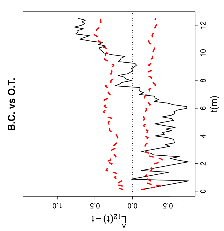
Figure 38: Ripley’s bivariate $L$-function $\widehat{L}_{12}(t)-t$ for the part of the swamp tree data we considered. Wide dashed lines are the upper and lower (pointwise) 95 % confidence bounds for the functions based on Monte Carlo simulations under the CSR independence pattern. B.C. = bald cypresses and O.T. = other trees.

10 Discussion

In this article, we consider the asymptotic distribution of the relative density of two proximity catch digraphs (PCDs), namely, proportional-edge PCDs and central similarity PCDs for testing bivariate spatial point patterns of segregation and association against complete spatial randomness (CSR). To our knowledge the PCD-based methods are the only graph theoretic tools for testing spatial point patterns in literature (Ceyhan and Priebe, (2005), Ceyhan et al., (2006), Ceyhan et al., (2007), and Ceyhan, 2010b ).

We first extend the expansion parameter of the central similarity PCD which was introduced in Ceyhan and Priebe, 2003a and Ceyhan et al., (2007) to values higher than one. We demonstrate that the relative density of the PCDs can be expressed as $U$-statistic of order 2 (in estimating the arc probability) and thereby prove the asymptotic normality of the relative density of the PCDs. For finite samples, we assess the empirical size and power of the relative density of the PCDs by extensive Monte Carlo simulations. For the proportional-edge PCDs, the optimal expansion parameters (in terms of appropriate empirical size and high power) are about 1.5 under mild segregation and values in $(2,3)$ under moderate to severe segregation; and about 2 under association. On the other hand, for central similarity PCDs, the optimal parameters are about 7 under segregation, and about 1 under association. Furthermore, we have shown that relative density of central similarity PCDs has better empirical size performance; and also, it has higher power against the segregation alternatives. On the other hand, relative density of proportional-edge PCDs has higher power against the association alternatives.

We also compare the asymptotic relative efficiency of the relative densities of the two PCD families. Based on Pitman asymptotic efficiency, we have shown that in general the relative density of proportional-edge PCDs is asymptotically more efficient under segregation, while relative density of central similarity PCDs is more efficient under association. However, for the above optimal expansion parameter values (optimal with respect to empirical size and power), the asymptotic efficiency and empirical power analysis yields the same ordering in terms of performance.

Let the two samples of sizes $n$ and $m$ be from classes $\mathcal{X}$ and $\mathcal{Y}$, respectively, with $\mathcal{X}$ points being used as the vertices of the PCDs and $\mathcal{Y}$ points being used in the construction of Delaunay triangulation. The null hypothesis is assumed to be CSR of $\mathcal{X}$ points, i.e., the uniformness of $\mathcal{X}$ points in the convex hull of $\mathcal{Y}$ points, $C_{H}(\mathcal{Y}_{m})$. Although we have two classes here, the null pattern is not the CSR independence, since for finite $m$, we condition on $m$ and the locations of the $\mathcal{Y}$ points (assumed to have no more than three co-circular points) are irrelevant. That is, the $\mathcal{Y}$ points can result from any pattern that results in a unique Delaunay triangulation. The relative density of the two PCD families lend themselves for spatial pattern testing conveniently, because of the geometry invariance property for uniform data on Delaunay triangles.

For the relative density approach to be appropriate, the size of $\mathcal{X}$ points (i.e., $n$) should be much larger compared to size of $\mathcal{Y}$ points (i.e., $m$). This implies that $n$ tends to infinity while $m$ is assumed to be fixed. That is, the imbalance in the relative abundance of the two classes should be large for our method to be appropriate. Such an imbalance usually confounds the results of other spatial interaction tests. Furthermore, by construction our method uses only the $\mathcal{X}$ points in $C_{H}(\mathcal{Y}_{m})$ which might cause substantial data (hence information) loss. To mitigate this, we propose a correction for the proportion of $\mathcal{X}$ points outside $C_{H}(\mathcal{Y}_{m})$, because the pattern inside $C_{H}(\mathcal{Y}_{m})$ might not be the same as the pattern outside $C_{H}(\mathcal{Y}_{m})$. We suggest a two-stage analysis with our relative density approach: (i) analysis for $C_{H}(\mathcal{Y}_{m})$, which provides inference restricted to $\mathcal{X}$ points in $C_{H}(\mathcal{Y}_{m})$, (ii) overall analysis with convex hull correction (i.e., for all $\mathcal{X}$ points with respect to $\mathcal{Y}_{m}$). We recommend the use of normal approximation if $n\approx 10\,m$ or more, although Monte Carlo simulations suggest smaller $n$ might also work fine.

There are many possible types of parameterizations for the alternatives. The particular parametrization of the alternatives in Equation (15) is chosen so that the distribution of the relative density under the alternatives would be geometry invariant also (i.e., independent of the geometry of the support triangles). The more natural alternatives (i.e., the alternatives that are more likely to be found in practice) can be similar to or might be approximated by our parametrization. Because under a segregation alternative, the $\mathcal{X}$ points will tend to be further away from $\mathcal{Y}$ points and under an association alternative $\mathcal{X}$ points will tend to cluster around the $\mathcal{Y}$ points. Such patterns can be detected by the test statistics based on the relative density, since under segregation (whether it is parametrized as in Section 4 or not) we expect them to be larger, and under association (regardless of the parametrization) they tend to be smaller.

APPENDIX

Appendix 1: Derivation of $\mu_{{}_{CS}}(\tau)$ and $\nu_{{}_{CS}}(\tau)$ for $\tau>1$

Let $M_{C}$ be the center of mass of the standard equilateral triangle $T_{e}$. By symmetry $\mu_{{}_{CS}}(\tau)=P\bigl{(}X_{2}\in N_{CS}(X_{1},\tau)\bigr{)}=6\,P\bigl{(}X_{2}\in N_{CS}(X_{1},\tau),\,X_{1}\in T(\mathsf{y}_{1},M_{3},M_{C})\bigr{)}$. To calculate this mean, we need to find the possible types of $N_{CS}(x_{1},\tau)$ for $\tau>1$. There are three cases regarding $N_{CS}(x_{1},\tau)$. See Figure 39 for the prototypes of these three cases of $N_{CS}(x_{1},\tau)$ for $x_{1}=(u_{1},v_{1})\in T(\mathcal{Y}_{3})$.

Each case $j$, corresponds to region $R_{j}$ in Figure 40, and the bounding lines are $r_{6}(x)$, $\ell_{am}(x)$, and $r_{7}(x)$ with $\ell_{am}(x)=x/\sqrt{3},\;\;\;r_{6}(x)={\frac{\sqrt{3}u_{1}}{1+2\,\tau}},\;\;\;r_{7}(x)=-{\frac{\sqrt{3}\left(-1+u_{1}\right)}{1+2\,\tau}}$ and $s_{2}=\frac{3}{2\,\left(2+\tau\right)}.$

The explicit forms of $R_{j}$, $j=1,2,3$ are as follows:

$$R_{1} =\bigl{\{}(x,y)\in[0,1/2]\times[0,r_{6}(x)]\bigr{\}},$$

$$R_{2} =\bigl{\{}(x,y)\in[0,s_{2}]\times[r_{6}(x),\ell_{am}(x)]\cup[s_{2},1/2]\times[r_{6}(x),r_{7}(x)]\bigr{\}},$$

$$R_{3} =\bigl{\{}(x,y)\in[s_{2},1/2]\times[r_{7}(x),\ell_{am}(x)]\bigr{\}}.$$

$$P\bigl{(}X_{2}\in N_{CS}(X_{1},\tau),\;X_{1}\in T_{s}\bigr{)}=\sum_{j=1}^{3}P\bigl{(}X_{2}\in N_{CS}(X_{1},\tau),\;X_{1}\in R_{j}\bigr{)}.$$

For $x_{1}\in R_{1}$,

$$P\bigl{(}X_{2}\in N_{CS}(X_{1},\tau),\;X_{1}\in R_{1}\bigr{)}=\int_{0}^{1/2}\int_{0}^{r_{6}(x)}\frac{A\left(N_{CS}(X_{1},\tau)\right)}{A(T(\mathcal{Y}_{3}))^{2}}dydx=\frac{1}{12\,\left(1+2\,\tau\right)},$$

where $A\left(N_{CS}(X_{1},\tau)\right)=\frac{1}{\sqrt{3}}\left(1+2\,\tau\right)^{2}v_{1}^{2}$.

For $x_{1}\in R_{2}$,

$$P\bigl{(}X_{2}\in N_{CS}(X_{1},\tau),\;X_{1}\in R_{2}\bigr{)}=\left(\int_{0}^{s_{2}}\int_{r_{6}(x)}^{\ell_{am}(x)}+\int_{s_{2}}^{1/2}\int_{r_{6}(x)}^{r_{7}(x)}\right)\frac{A\left(N_{CS}(X_{1},\tau)\right)^{2}}{A(T(\mathcal{Y}_{3}))^{3}}dydx={\frac{\tau-1}{2\left(1+2\,\tau\right)\left(2+\tau\right)}}.$$

where $A\left(N_{CS}(X_{1},\tau)\right)=\frac{\sqrt{3}}{12}\,\left(v_{1}+2\,\tau\,v_{1}+\sqrt{3}u_{1}\right)^{2}$.

For $x_{1}\in R_{3}$,

$$P\bigl{(}X_{2}\in N_{CS}(X_{1},\tau),\;X_{1}\in R_{3}\bigr{)}=\int_{s_{2}}^{1/2}\int_{r_{7}(x)}^{\ell_{am}(x)}\frac{A\left(N_{CS}(X_{1},\tau)\right)}{A(T(\mathcal{Y}_{3}))^{2}}dydx={\frac{\left(\tau-1\right)^{2}}{3\left(1+2\,\tau\right)\left(2+\tau\right)}}.$$

where $A\left(N_{CS}(X_{1},\tau)\right)=\frac{\sqrt{3}}{4}$.

So $P\bigl{(}X_{2}\in N_{CS}(X_{1},\tau)\bigr{)}={\frac{\tau\,\left(4\,\tau-1\right)}{2\,\left(1+2\,\tau\right)\left(2+\tau\right)}}.$

Next, we find the asymptotic variance term. Let

$$P^{2N}_{{}_{CS}}:=P\bigl{(}\{X_{2},X_{3}\}\subset N_{CS}(X_{1},\tau)\bigr{)},\;\;\;P^{2G}_{{}_{CS}}:=P\bigl{(}\{X_{2},X_{3}\}\subset\Gamma_{1}^{{}^{CS}}(X_{1},\tau)\bigr{)}\;\;\text{ and }\;\;$$

$$P^{M}_{{}_{CS}}:=P\bigl{(}X_{2}\in N_{CS}(X_{1},\tau),X_{3}\in\Gamma_{1}^{{}^{CS}}(X_{1},\tau)\bigr{)}.$$

where $\Gamma_{1}^{{}^{CS}}(x,\tau)$ is the $\Gamma_{1}$-region of $x$ based on $N_{CS}(\cdot,\tau)$ and defined as $\Gamma_{1}^{{}^{CS}}(x,\tau):=\{y\in T(\mathcal{Y}_{3}):\;x\subset N_{CS}(y,\tau)\}$. See Ceyhan and Priebe, 2003b for more detail.

Then $\mathbf{Cov}[h_{12},h_{13}]=\mathbf{E}[h_{12}\,h_{13}]-\mathbf{E}[h_{12}]\mathbf{E}[h_{13}]$ where

$$\mathbf{E}[h_{12}\,h_{13}] = P\bigl{(}\{X_{2},X_{3}\}\subset N_{CS}(X_{1},\tau)\bigr{)}+2\,P\bigl{(}X_{2}\in N_{CS}(X_{1},\tau),X_{3}\in\Gamma_{1}^{{}^{CS}}(X_{1},\tau)\bigr{)}$$

$$+P\bigl{(}\{X_{2},X_{3}\}\subset\Gamma_{1}^{{}^{CS}}(X_{1},\tau)\bigr{)}=P^{2N}_{{}_{CS}}+2\,P^{M}_{{}_{CS}}+P^{2G}_{{}_{CS}}.$$

Hence $\nu_{{}_{CS}}(\tau)=\mathbf{Cov}[h_{12},h_{13}]=\bigl{(}P^{2N}_{{}_{CS}}+2\,P^{M}_{{}_{CS}}+P^{2G}_{{}_{CS}}\bigr{)}-[2\,\mu_{{}_{CS}}(\tau)]^{2}.$

To find the covariance, we need to find the possible types of $\Gamma_{1}^{{}^{CS}}(x_{1},\tau)$ and $N_{CS}(x_{1},\tau)$ for $\tau\in(1,\infty)$. There are three cases regarding $N_{CS}(x_{1},\tau)$ and one case for $\Gamma_{1}^{{}^{CS}}(x_{1},\tau)$. See Figure 40 for the prototype of this one case of $\Gamma_{1}^{{}^{CS}}(x_{1},\tau)$ for $x_{1}=(u_{1},v_{1})\in T(\mathcal{Y}_{3})$, the explicit forms of $\zeta_{j}(\tau,x)$ are

$$\zeta_{1}(\tau,x) =\frac{\left(\sqrt{3}\,v_{1}+3\,u_{1}-3\,x\right)}{\sqrt{3}\,(1+2\,\tau)},\;\;\zeta_{2}(\tau,x)=-\frac{\left(-\sqrt{3}\,v_{1}+3\,u_{1}-3\,x\right)}{\sqrt{3}\,(1+2\,\tau)},$$

$$\zeta_{3}(\tau,x) =\frac{\left(3\,u_{1}+3\,\tau-3\,\tau\,x-3\,x-\sqrt{3}\,v_{1}\right)}{\sqrt{3}\,(-1+\tau)},\;\;\;\zeta_{4}(\tau,x)=-\frac{-\sqrt{3}\,\tau+\sqrt{3}\,\tau\,x-2\,v_{1}}{2+\tau},$$

$$\zeta_{5}(\tau,x) =\frac{\sqrt{3}\,\tau\,x+2\,v_{1}}{2+\tau},\;\;\;\zeta_{6}(\tau,x)=\frac{\left(-3\,x-3\,\tau\,x+3\,u_{1}+\sqrt{3}\,v_{1}\right)}{\sqrt{3}\,(1-\tau)},\;\;\;\zeta_{7}(\tau,x)=\frac{v_{1}}{1-\tau}.$$

Figure 39: The prototypes of the three cases of $N_{CS}(x_{1},\tau)$ for $x_{1}\in T(\mathsf{y}_{1},M_{3},M_{C})$ with $\tau=2.5$.

Figure 40: The regions corresponding to the prototypes of the four cases (left) and the prototype of the one case of $\Gamma_{1}^{{}^{CS}}(x_{1},\tau)$ for $x_{1}\in T(\mathsf{y}_{1},M_{3},M_{C})$ (right) with $\tau=2.5$.

By symmetry, $P^{2N}_{{}_{CS}}=6\,P\bigl{(}\{X_{2},X_{3}\}\subset N_{CS}(X_{1},\tau),\;X_{1}\in T_{s}\bigr{)},$ and

$$P\bigl{(}\{X_{2},X_{3}\}\subset N_{CS}(X_{1},\tau),\;X_{1}\in T_{s}\bigr{)}=\sum_{j=1}^{3}P\bigl{(}\{X_{2},X_{3}\}\subset N_{CS}(X_{1},\tau),\;X_{1}\in R_{j}\bigr{)}.$$

The limits of integration are as in $P\bigl{(}X_{2}\in N_{CS}(X_{1},\tau),\,X_{1}\in T_{s}\bigr{)}$ with the integrand being $\frac{A(N_{CS}(x_{1},\tau))^{2}}{A(T(\mathcal{Y}_{3}))^{3}}$. Hence, $P^{2N}_{{}_{CS}}={\frac{10\,\tau^{2}-9\,\tau+2}{5\,\left(2\,\tau+1\right)\left(\tau+2\right)}}.$

Next, by symmetry, $P^{2G}_{{}_{CS}}=6\,P\bigl{(}\{X_{2},X_{3}\}\subset\Gamma_{1}^{{}^{CS}}(X_{1},\tau),\;X_{1}\in T_{s}\bigr{)},$ and

$$P\bigl{(}\{X_{2},X_{3}\}\subset\Gamma_{1}^{{}^{CS}}(X_{1},\tau),\;X_{1}\in T_{s}\bigr{)}=\int_{0}^{1/2}\int_{0}^{\ell_{am}(x)}\frac{A\left(\Gamma_{1}^{{}^{CS}}(x_{1},\tau)\right)^{2}}{A(T(\mathcal{Y}_{3}))^{3}}dydx={\frac{\tau^{2}\left(10\,\tau^{2}-5\,\tau+1\right)}{15\,\left(2\,\tau+1\right)^{2}\left(\tau+2\right)^{2}}},$$

where $A\left(\Gamma_{1}^{{}^{CS}}(x_{1},\tau)\right)={\frac{\sqrt{3}\left(3\,u_{1}+\sqrt{3}v_{1}+\tau-1-3\,v_{1}^{2}-3\,u_{1}^{2}\right)\tau}{2\,\left(2\,\tau+1\right)\left(\tau+2\right)}}$.

So $P^{2G}_{{}_{CS}}={\frac{2\,\tau^{2}\left(10\,\tau^{2}-5\,\tau+1\right)}{5\,\left(2\,\tau+1\right)^{2}\left(\tau+2\right)^{2}}}.$

Furthermore, by symmetry, $P^{M}_{{}_{CS}}=6\,P\bigl{(}X_{2}\in N_{CS}(X_{1},\tau),\;X_{3}\in\Gamma_{1}^{{}^{CS}}(X_{1},\tau),\;X_{1}\in T_{s}\bigr{)},$ and

$$P\bigl{(}X_{2}\in N_{CS}(X_{1},\tau),\;X_{3}\in\Gamma_{1}^{{}^{CS}}(X_{1},\tau),\;X_{1}\in T_{s}\bigr{)}=\sum_{j=1}^{3}P\left(X_{2}\in N_{CS}(X_{1},\tau),\;X_{3}\in\Gamma_{1}^{{}^{CS}}(X_{1},\tau),\;X_{1}\in R_{j}\right).$$

where $P\bigl{(}X_{2}\in N_{CS}(X_{1},\tau),\;X_{3}\in\Gamma_{1}^{{}^{CS}}(X_{1},\tau),\;X_{1}\in R_{j}\bigr{)}$ can be calculated with the same region of integration with integrand being replaced by $\frac{A(N_{CS}(x_{1},\tau))\,A\left(\Gamma_{1}^{{}^{CS}}(x_{1},\tau)\right)}{A(T(\mathcal{Y}_{3}))^{3}}$.

Then $P^{M}_{{}_{CS}}={\frac{\tau^{2}\left(10-54\,\tau-99\,\tau^{2}+388\,\tau^{3}+1062\,\tau^{4}+720\,\tau^{5}+160\,\tau^{6}\right)}{10\,\left(2\,\tau+1\right)^{4}\left(\tau+2\right)^{4}}}.$

Hence

$$\mathbf{E}[h_{12}\,h_{13}]={\frac{2\,(160\,\tau^{8}-265\,\tau^{3}-135\,\tau^{4}+751\,\tau^{5}-47\,\tau^{2}+1373\,\tau^{6}+804\,\tau^{7}+24\,\tau+8)}{5\,\left(2\,\tau+1\right)^{4}\left(\tau+2\right)^{4}}}.$$

Therefore,

$$\nu_{{}_{CS}}(\tau)={\frac{168\,\tau^{7}+886\,\tau^{6}+1122\,\tau^{5}+45\,\tau^{4}-470\,\tau^{3}-114\,\tau^{2}+48\,\tau+16}{5\,\left(2\,\tau+1\right)^{4}\left(\tau+2\right)^{4}}}.$$

For $\tau=\infty$, it is trivial to see that $\nu_{{}_{CS}}(\tau)=0$.

Appendix 2: Derivation of $\mu^{S}_{{}_{CS}}(\tau,\varepsilon)$ for $\tau>1$

We pick the interval $\varepsilon\in\bigl{[}0,\sqrt{3}/5\bigr{)}$ for a demonstrative example in derivation of $\mu^{S}_{{}_{CS}}(\tau,\varepsilon)$. For $\tau\in\bigl{[}1-\sqrt{3}\,\varepsilon,1\bigr{)}$, there are seven cases to consider for the form of $N_{CS}(\cdot,\tau)(x_{1},\varepsilon)$. See Figure 41 for the prototypes of these seven cases of $N_{CS}(\cdot,\tau)(x_{1},\varepsilon)$.

Figure 41: The seven possible cases of $N_{CS}(\cdot,\tau)(x)$ for four distinct $x\in R_{CM}(e_{3})$ (shaded regions).

Each case $j$, corresponds to the region $R_{j}$ in Figure 42, where $q_{1}(x)=-\sqrt{3}\,x+2\,\varepsilon,\;\;\;q_{2}(x)=\frac{-\sqrt{3}\,x+2\,\varepsilon}{1-4\,\tau},\;\;\;q_{3}(x)=\frac{\sqrt{3}\,x+2\,\varepsilon-\sqrt{3}}{1-4\,\tau},\;\;\;q_{4}(x)=\frac{\sqrt{3}-2\,\varepsilon}{2\,(1+2\,\tau)}$ and $s_{1}=\sqrt{3}\,\varepsilon/2,\;\;\;s_{2}=2\,\sqrt{3}\,\varepsilon/3,\;\;\;s_{3}=\frac{\sqrt{3}\,(\sqrt{3}-2\,\varepsilon)}{2\,(1+2\,\tau)}.$

Figure 42: The regions corresponding to the prototypes of the seven cases shown in Figure 41.

The explicit forms of $R_{j}$, $j=1,2,\ldots,7$ are as follows:

$$R_{1} =\bigl{\{}(x,y)\in[s_{3},1/2]\times[0,r_{1}(x)]\bigr{\}},$$

$$R_{2} =\bigl{\{}(x,y)\in[s_{2},s_{3}]\times[\ell_{16}(x),r_{6}(x)]\cup[s_{3},s_{7}]\times[r_{1}(x),r_{6}(x)]\cup[s_{7},1/2]\times[r_{1}(x),r_{2}(x)]\bigr{\}},$$

$$R_{3} =\bigl{\{}(x,y)\in[s_{7},1/2]\times[r_{2}(x),r_{3}(x)]\bigr{\}},$$

$$R_{4} =\bigl{\{}(x,y)\in[s_{7},1/2]\times[r_{3}(x),r_{6}(x)]\bigr{\}},$$

$$R_{5} =\bigl{\{}(x,y)\in[s_{1},s_{2}]\times[\ell_{16}(x),\ell_{am}(x)]\cup[s_{2},s_{5}]\times[r_{6}(x),\ell_{am}(x)]\cup[s_{5},s_{7}]\times[r_{6}(x),r_{2}(x)]\bigr{\}},$$

$$R_{6} =\bigl{\{}(x,y)\in[s_{5},s_{6}]\times[r_{2}(x),\ell_{am}(x)]\cup[s_{6},s_{7}]\times[r_{2}(x),r_{7}(x)]\cup[s_{7},1/2]\times[r_{6}(x),r_{7}(x)]\bigr{\}},$$

$$R_{7} =\bigl{\{}(x,y)\in[s_{6},1/2]\times[r_{7}(x),\ell_{am}(x)]\bigr{\}}.$$

By symmetry, $P\bigl{(}X_{2}\in N_{CS}(X_{1},\tau,\varepsilon)\bigr{)}=6\,P\bigl{(}X_{2}\in N_{CS}(X_{1},\tau,\varepsilon),\;X_{1}\in T_{s}\bigr{)}.$

For $x_{1}\in R_{1}$,

$$P\bigl{(}X_{2}\in N_{CS}(X_{1},\tau,\varepsilon),\;X_{1}\in R_{1}\bigr{)}=\int_{s_{3}}^{1/2}\int_{0}^{r_{1}(x)}\frac{A(N_{CS}(X_{1},\tau,\varepsilon))^{2}}{A(T(\mathcal{Y}_{3}))^{2}}dydx={\frac{9+256\,\varepsilon^{4}-48\,\varepsilon\,\sqrt{3}+288\,\varepsilon^{2}-256\,\varepsilon^{3}\sqrt{3}}{108\,\left(1+2\,\tau\right)\left(4\,\varepsilon^{2}-1\right)^{2}}},$$

where $A\left(N_{CS}(X_{1},\tau,\varepsilon)\right)=\frac{1}{\sqrt{3}}\left(1+2\,\tau\right)^{2}v_{1}^{2}$.

For $x_{1}\in R_{2}$,

$$P\bigl{(}X_{2}\in N_{CS}(X_{1},\tau,\varepsilon),\;X_{1}\in R_{2}\bigr{)}=\left(\int_{s_{2}}^{s_{3}}\int_{\ell_{16}(x)}^{r_{6}(x)}+\int_{s_{3}}^{s_{7}}\int_{r_{1}(x)}^{r_{6}(x)}+\int_{s_{7}}^{1/2}\int_{r_{1}(x)}^{r_{2}(x)}\right)\frac{A(N_{CS}(X_{1},\tau,\varepsilon))^{2}}{A(T(\mathcal{Y}_{3}))^{2}}dydx=\\ \Big{[}4\,\varepsilon\,\Big{(}3\,\sqrt{3}-27\,\varepsilon+9\,\sqrt{3}\tau-16\,\varepsilon^{3}+24\,\varepsilon^{2}\sqrt{3}-24\,\varepsilon^{3}\tau^{3}-48\,\varepsilon^{3}\tau-54\,\varepsilon^{3}\tau^{2}-27\,\varepsilon\,\tau^{3}-81\,\tau\,\varepsilon-81\,\varepsilon\,\tau^{2}+\\ 9\,\sqrt{3}\tau^{2}+3\,\sqrt{3}\tau^{3}+72\,\varepsilon^{2}\sqrt{3}\tau+72\,\varepsilon^{2}\sqrt{3}\tau^{2}+24\,\varepsilon^{2}\sqrt{3}\tau^{3}\Big{)}\Big{]}\Big{/}\Big{[}27\,\left(1+\tau\right)^{3}\left(1+2\,\tau\right)\left(4\,\varepsilon^{2}-1\right)^{2}\Big{]},$$

where $A\left(N_{CS}(X_{1},\tau,\varepsilon)\right)=\frac{\sqrt{3}}{12}\left(-2\,\varepsilon+v_{1}+2\,\tau\,v_{1}+\sqrt{3}u_{1}\right)\left(2\,\varepsilon-\sqrt{3}u_{1}+3\,v_{1}+6\,\tau\,v_{1}\right)$.

For $x_{1}\in R_{3}$,

$$P\bigl{(}X_{2}\in N_{CS}(X_{1},\tau,\varepsilon),\;X_{1}\in R_{3}\bigr{)}=\int_{s_{7}}^{1/2}\int_{r_{2}(x)}^{r_{3}(x)}\frac{A(N_{CS}(X_{1},\tau,\varepsilon))^{2}}{A(T(\mathcal{Y}_{3}))^{2}}dydx={\frac{2\,\varepsilon^{2}\left(9+18\,\varepsilon^{2}-16\,\varepsilon\,\sqrt{3}\right)}{27\,\left(1+2\,\tau\right)\left(4\,\varepsilon^{2}-1\right)^{2}}},$$

where

$$A\left(N_{CS}(X_{1},\tau,\varepsilon)\right)=\frac{\sqrt{3}}{12}\left(4\,\varepsilon\,\sqrt{3}-3+4\,\sqrt{3}\tau\,v_{1}+6\,u_{1}+2\,\sqrt{3}v_{1}-8\,\varepsilon^{2}-16\,\varepsilon\,\tau\,v_{1}+2\,v_{1}^{2}-8\,\varepsilon\,v_{1}+8\,\tau\,v_{1}^{2}+8\,\tau^{2}v_{1}^{2}-6\,u_{1}^{2}\right).$$

For $x_{1}\in R_{4}$,

$$P\bigl{(}X_{2}\in N_{CS}(X_{1},\tau,\varepsilon),\;X_{1}\in R_{4}\bigr{)}=\int_{s_{7}}^{1/2}\int_{r_{3}(x)}^{r_{6}(x)}\frac{A(N_{CS}(X_{1},\tau,\varepsilon))^{2}}{A(T(\mathcal{Y}_{3}))^{2}}dydx={\frac{2\,\varepsilon^{2}\left(9-8\,\varepsilon\,\sqrt{3}-8\,\varepsilon^{2}\right)}{27\,\left(1+2\,\tau\right)\left(4\,\varepsilon^{2}-1\right)^{2}}},$$

where

$$A\left(N_{CS}(X_{1},\tau,\varepsilon)\right)=\frac{\sqrt{3}}{6}\left(4\,\varepsilon\,\sqrt{3}-3+6\,\sqrt{3}\tau\,v_{1}+3\,u_{1}+3\,\sqrt{3}v_{1}-6\,\varepsilon^{2}-16\,\varepsilon\,\tau\,v_{1}-v_{1}^{2}-8\,\varepsilon\,v_{1}-4\,\tau\,v_{1}^{2}-4\,\tau^{2}v_{1}^{2}-3\,u_{1}^{2}\right).$$

For $x_{1}\in R_{5}$,

$$P\bigl{(}X_{2}\in N_{CS}(X_{1},\tau,\varepsilon),\;X_{1}\in R_{5}\bigr{)}=\left(\int_{s_{1}}^{s_{2}}\int_{\ell_{16}(x)}^{\ell_{am}(x)}+\int_{s_{2}}^{s_{5}}\int_{r_{6}(x)}^{\ell_{am}(x)}+\int_{s_{5}}^{s_{7}}\int_{r_{6}(x)}^{r_{2}(x)}\right)\frac{A(N_{CS}(X_{1},\tau,\varepsilon))^{2}}{A(T(\mathcal{Y}_{3}))^{2}}dydx=\\ \Big{[}27\,\tau^{4}-4\,\varepsilon^{4}\tau^{7}-46\,\varepsilon^{4}\tau^{6}-130\,\varepsilon^{4}\tau^{5}-72\,\varepsilon\,\sqrt{3}\tau^{4}+144\,\varepsilon^{2}\tau^{4}-74\,\varepsilon^{4}\tau^{4}+288\,\varepsilon^{2}\tau^{3}+54\,\tau^{3}+142\,\varepsilon^{4}\tau^{3}-144\,\varepsilon\,\sqrt{3}\tau^{3}+112\,\tau^{2}\varepsilon^{4}-\\ 54\,\tau+144\,\tau\,\varepsilon\,\sqrt{3}-288\,\varepsilon^{2}\tau-27+72\,\varepsilon\,\sqrt{3}-144\,\varepsilon^{2}\Big{]}\Big{/}\Big{[}54\,\left(4\,\varepsilon^{2}-1\right)^{2}\left(1+2\,\tau\right)\left(2+\tau\right)\left(1+\tau\right)^{3}\Big{]},$$

where $A\left(N_{CS}(X_{1},\tau,\varepsilon)\right)=\frac{\sqrt{3}}{12}\left(-2\,\varepsilon+v_{1}+2\,\tau\,v_{1}+\sqrt{3}u_{1}\right)\left(\sqrt{3}u_{1}+v_{1}+2\,\tau\,v_{1}+2\,\varepsilon\right)$.

For $x_{1}\in R_{6}$,

$$P\bigl{(}X_{2}\in N_{CS}(X_{1},\tau,\varepsilon),\;X_{1}\in R_{6}\bigr{)}=\left(\int_{s_{5}}^{s_{6}}\int_{r_{2}(x)}^{\ell_{am}(x)}+\int_{s_{6}}^{s_{7}}\int_{r_{2}(x)}^{r_{7}(x)}+\int_{s_{7}}^{1/2}\int_{r_{6}(x)}^{r_{7}(x)}\right)\frac{A(N_{CS}(X_{1},\tau,\varepsilon))^{2}}{A(T(\mathcal{Y}_{3}))^{2}}dydx=\\ \Big{[}4\,\left(10\,\varepsilon^{3}\tau+9\,\sqrt{3}\tau-27\,\tau\,\varepsilon-8\,\varepsilon^{2}\sqrt{3}\tau-10\,\varepsilon^{3}-9\,\sqrt{3}+27\,\varepsilon+8\,\varepsilon^{2}\sqrt{3}\right)\varepsilon\Big{]}\Big{/}\Big{[}27\,\left(2+\tau\right)\left(1+2\,\tau\right)\left(4\,\varepsilon^{2}-1\right)^{2}\Big{]},$$

where

$$A\left(N_{CS}(X_{1},\tau,\varepsilon)\right)=\frac{\sqrt{3}}{12}\Big{(}4\,\sqrt{3}v_{1}-8\,\varepsilon\,v_{1}+8\,\sqrt{3}\tau\,v_{1}-16\,\varepsilon\,\tau\,v_{1}+12\,u_{1}-8\,\varepsilon\,\sqrt{3}u_{1}-6+8\,\varepsilon\,\sqrt{3}-12\,\varepsilon^{2}-v_{1}^{2}-4\,\tau\,v_{1}^{2}-\\ 2\,\sqrt{3}u_{1}\,v_{1}-4\,\sqrt{3}u_{1}\,\tau\,v_{1}-3\,u_{1}^{2}-4\,\tau^{2}v_{1}^{2}\Big{)}.$$

For $x_{1}\in R_{7}$,

$$P\bigl{(}X_{2}\in N_{CS}(X_{1},\tau,\varepsilon),\;X_{1}\in R_{7}\bigr{)}=\int_{s_{7}}^{1/2}\int_{r_{3}(x)}^{r_{6}(x)}\frac{A(N_{CS}(X_{1},\tau,\varepsilon))^{2}}{A(T(\mathcal{Y}_{3}))^{2}}dydx={\frac{1-2\,\tau+\tau^{2}}{3\,\left(1-4\,\varepsilon^{2}\right)\left(1+2\,\tau\right)\left(2+\tau\right)}},$$

where $A\left(N_{CS}(X_{1},\tau,\varepsilon)\right)=\frac{\sqrt{3}}{4}\left(2\,\varepsilon+1\right)\left(1-2\,\varepsilon\right)$.

So

$$P\bigl{(}X_{2}\in N_{CS}(X_{1},\tau,\varepsilon)\bigr{)}=\Big{[}\Big{(}36\,\tau^{3}-8\,\varepsilon^{4}\tau^{5}-84\,\varepsilon^{4}\tau^{4}-144\,\varepsilon^{2}\tau^{3}-176\,\varepsilon^{4}\tau^{3}-192\,\tau^{2}\sqrt{3}\varepsilon^{3}+63\,\tau^{2}+140\,\tau^{2}\varepsilon^{4}-144\,\varepsilon^{2}\tau^{2}-\\ 384\,\sqrt{3}\tau\,\varepsilon^{3}+18\,\tau+512\,\varepsilon^{4}\tau+144\,\varepsilon^{2}\tau-9-192\,\varepsilon^{3}\sqrt{3}+144\,\varepsilon^{2}+240\,\varepsilon^{4}\Big{)}\tau\Big{]}\Big{/}\Big{[}18\,\left(1+\tau\right)^{2}\left(2+\tau\right)\left(1+2\,\tau\right)\left(4\,\varepsilon^{2}-1\right)^{2}\Big{]}.$$

Appendix 3: The Mean $\mu^{S}_{{}_{CS}}(\tau,\varepsilon)$ under the Segregation and Association Alternatives

Derivation of $\mu^{S}_{{}_{CS}}(\tau,\varepsilon)$ involves detailed geometric calculations and partitioning of the space of $(\tau,\varepsilon,x_{1})$ for $\tau\in[0,1]$, $\varepsilon\in\bigl{[}0,\sqrt{3}/3\bigr{)}$, and $x_{1}\in T_{s}=T(\mathsf{y}_{1},M_{3},M_{C})$. A demonstrative calculation is given in Appendix 2 for $\varepsilon\in[0,\sqrt{3}/5)$ and $\tau\in[1-\sqrt{3}\,\varepsilon,1]$.

$\mu^{S}_{{}_{CS}}(\tau,\varepsilon)$ under the Segregation Alternatives

Under segregation, we compute $\mu^{S}_{{}_{CS}}(\tau,\varepsilon)$ explicitly. For $\varepsilon\in[0,\sqrt{3}/5)$,

$$\mu^{S}_{{}_{CS}}(\tau,\varepsilon)=\sum_{j=1}^{2}\varpi_{1,j}(\tau,\varepsilon)\,\mathbf{I}(\tau\in\mathcal{I}_{j})$$

where

$$\varpi_{1,1}(\tau,\varepsilon) =\frac{(20\,\varepsilon^{4}\tau-36\,\varepsilon^{4}-3\,\tau+3)\tau^{2}}{18\,(1-\tau)(2\,\varepsilon+1)^{2}(2\,\varepsilon-1)^{2}},$$

$$\varpi_{1,2}(\tau,\varepsilon) =-\Bigl{[}\Bigl{(}80\,\varepsilon^{4}\tau^{3}+16\,\varepsilon^{4}\tau^{2}-108\,\varepsilon^{4}\tau-144\,\varepsilon^{4}+192\,\sqrt{3}\varepsilon^{3}+288\,\varepsilon^{2}\tau+64\,\sqrt{3}\,\varepsilon\,\tau^{2}+4\,\tau^{3}$$

$$-288\,\varepsilon^{2}-128\,\sqrt{3}\,\varepsilon\,\tau-60\,\tau^{2}+64\,\sqrt{3}\,\varepsilon+45\,\tau-16\Bigr{)}\tau\Bigr{]}\Big{/}\bigl{[}18\,(2\,\tau+1)^{2}(2\,\varepsilon-1)^{2}(2\,\varepsilon+1)^{2}\bigr{]},$$

with the corresponding intervals $\mathcal{I}_{1}=\bigl{[}1,1-\sqrt{3}\,\varepsilon\bigr{)}$ and $\mathcal{I}_{2}=\bigl{[}1-\sqrt{3}\,\varepsilon,1\bigr{)}$.

For $\varepsilon\in\bigl{[}\sqrt{3}/5,\sqrt{3}/4\bigr{)}$,

$$\mu^{S}_{{}_{CS}}(\tau,\varepsilon)=\sum_{j=1}^{3}\varpi_{2,j}(\tau,\varepsilon)\,\mathbf{I}(\tau\in\mathcal{I}_{j})$$

where $\varpi_{2,j}(\tau,\varepsilon)=\varpi_{1,j}(\tau,\varepsilon)$ for $j=1,2$, and for $j=3$,

$$\varpi_{2,3}(\tau,\varepsilon)=\Bigl{[}\Bigl{(}-96\,\varepsilon^{4}\tau^{4}-1584\,\varepsilon^{4}\tau^{3}-3688\,\varepsilon^{4}\tau^{2}+512\,\sqrt{3}\varepsilon^{3}\tau^{3}-3636\,\varepsilon^{4}\tau+2304\,\sqrt{3}\varepsilon^{3}\tau^{2}-1152\,\varepsilon^{4}+3840\,\sqrt{3}\varepsilon^{3}\tau-576\,\varepsilon^{2}\tau^{2}+\\ 128\,\sqrt{3}\,\varepsilon\,\tau^{3}+8\,\tau^{4}+1536\,\sqrt{3}\varepsilon^{3}-4320\,\varepsilon^{2}\tau-320\,\sqrt{3}\,\varepsilon\,\tau^{2}-124\,\tau^{3}-2304\,\varepsilon^{2}+640\,\sqrt{3}\,\varepsilon\,\tau+150\,\tau^{2}+512\,\sqrt{3}\,\varepsilon-\\ 77\,\tau-128\Bigr{)}\tau\Bigr{]}\Big{/}\Bigl{[}18\,(2\,\tau+1)^{2}(2\,\varepsilon-1)^{2}(2\,\varepsilon+1)^{2}(1-2\,\tau)\Bigr{]},$$

with the corresponding intervals $\mathcal{I}_{1}=\bigl{[}1,1-\sqrt{3}\,\varepsilon\bigr{)}$, $\mathcal{I}_{2}=\bigl{[}1-\sqrt{3}\,\varepsilon,\sqrt{3}/(2\,\varepsilon)-3/2\bigr{)}$, and $\mathcal{I}_{3}=\bigl{[}\sqrt{3}/(2\,\varepsilon)-3/2,1\bigr{)}$.

For $\varepsilon\in\bigl{[}\sqrt{3}/4,2\,\sqrt{3}/7\bigr{)}$, $\mu^{S}_{{}_{CS}}(\tau,\varepsilon)=\sum_{j=1}^{5}\varpi_{3,j}(\tau,\varepsilon)\,\mathbf{I}(\tau\in\mathcal{I}_{j})$ where

$$\varpi_{3,1}(\tau,\varepsilon)=\Bigl{[}(984\,\varepsilon^{4}\tau^{3}-3452\,\varepsilon^{4}\tau^{2}-1024\,\sqrt{3}\varepsilon^{3}\tau^{3}+4992\,\varepsilon^{4}\tau+3584\,\sqrt{3}\varepsilon^{3}\tau^{2}+1152\,\varepsilon^{2}\tau^{3}-2268\,\varepsilon^{4}-5120\,\sqrt{3}\varepsilon^{3}\tau-4032\,\varepsilon^{2}\tau^{2}-\\ 192\,\sqrt{3}\,\varepsilon\,\tau^{3}+2304\,\sqrt{3}\varepsilon^{3}+5760\,\varepsilon^{2}\tau+672\,\sqrt{3}\,\varepsilon\,\tau^{2}+42\,\tau^{3}-2592\,\varepsilon^{2}-960\,\sqrt{3}\,\varepsilon\,\tau-141\,\tau^{2}+432\,\sqrt{3}\,\varepsilon+192\,\tau-84)\tau^{2}\Bigr{]}\Big{/}\\ \Bigl{[}32\,(\tau-1)^{2}\left(3\,\varepsilon-\sqrt{3}\right)^{4}(2\,\tau-1)\Bigr{]},$$

$$\varpi_{3,2}(\tau,\varepsilon)=\Bigl{[}(3936\,\varepsilon^{4}\tau^{6}-9872\,\varepsilon^{4}\tau^{5}-4096\,\sqrt{3}\varepsilon^{3}\tau^{6}+7144\,\varepsilon^{4}\tau^{4}+10240\,\sqrt{3}\varepsilon^{3}\tau^{5}+4608\,\varepsilon^{2}\tau^{6}+7444\,\varepsilon^{4}\tau^{3}-7168\,\sqrt{3}\varepsilon^{3}\tau^{4}-\\ 11520\,\varepsilon^{2}\tau^{5}-768\,\sqrt{3}\,\varepsilon\,\tau^{6}-4368\,\varepsilon^{4}\tau^{2}-8064\,\sqrt{3}\varepsilon^{3}\tau^{3}+7488\,\varepsilon^{2}\tau^{4}+1792\,\sqrt{3}\,\varepsilon\,\tau^{5}+136\,\tau^{6}-1836\,\varepsilon^{4}\tau+5056\,\sqrt{3}\varepsilon^{3}\tau^{2}+\\ 10656\,\varepsilon^{2}\tau^{3}-768\,\sqrt{3}\,\varepsilon\,\tau^{4}-220\,\tau^{5}-144\,\varepsilon^{4}+1536\,\sqrt{3}\varepsilon^{3}\tau-7200\,\varepsilon^{2}\tau^{2}-2464\,\sqrt{3}\,\varepsilon\,\tau^{3}-154\,\tau^{4}+192\,\sqrt{3}\varepsilon^{3}-1152\,\varepsilon^{2}\tau+\\ 1664\,\sqrt{3}\,\varepsilon\,\tau^{2}+771\,\tau^{3}-288\,\varepsilon^{2}+48\,\sqrt{3}\,\varepsilon\,\tau-464\,\tau^{2}+64\,\sqrt{3}\,\varepsilon+28\,\tau-16)\tau\Bigr{]}\Big{/}\Bigl{[}32\,\left(3\,\varepsilon-\sqrt{3}\right)^{4}(2\,\tau-1)(2\,\tau+1)^{2}(\tau-1)^{2}\Bigr{]},$$

$$\varpi_{3,3}(\tau,\varepsilon)=\Bigl{[}(2096\,\varepsilon^{4}\tau^{5}-3376\,\varepsilon^{4}\tau^{4}-2048\,\sqrt{3}\varepsilon^{3}\tau^{5}+2204\,\varepsilon^{4}\tau^{3}+3840\,\sqrt{3}\varepsilon^{3}\tau^{4}+2304\,\varepsilon^{2}\tau^{5}+3864\,\varepsilon^{4}\tau^{2}-2304\,\sqrt{3}\varepsilon^{3}\tau^{3}-\\ 4608\,\varepsilon^{2}\tau^{4}-384\,\sqrt{3}\,\varepsilon\,\tau^{5}-1332\,\varepsilon^{4}\tau-4864\,\sqrt{3}\varepsilon^{3}\tau^{2}+2016\,\varepsilon^{2}\tau^{3}+704\,\sqrt{3}\,\varepsilon\,\tau^{4}+68\,\tau^{5}-1152\,\varepsilon^{4}+1536\,\sqrt{3}\varepsilon^{3}\tau+6912\,\varepsilon^{2}\tau^{2}-32\,\sqrt{3}\,\varepsilon\,\tau^{3}-\\ 76\,\tau^{4}+1536\,\sqrt{3}\varepsilon^{3}-1728\,\varepsilon^{2}\tau-1440\,\sqrt{3}\,\varepsilon\,\tau^{2}-115\,\tau^{3}-2304\,\varepsilon^{2}+208\,\sqrt{3}\,\varepsilon\,\tau+328\,\tau^{2}+512\,\sqrt{3}\,\varepsilon+4\,\tau-128)\tau\Bigr{]}\Big{/}\Bigl{[}32\,(\tau-1)^{2}\\ \left(-3\,\varepsilon+\sqrt{3}\right)^{4}(2\,\tau+1)^{2}\Bigr{]},$$

$$\varpi_{3,4}(\tau,\varepsilon)=\Bigl{[}(2064\,\varepsilon^{4}\tau^{6}-1696\,\varepsilon^{4}\tau^{5}-2048\,\sqrt{3}\varepsilon^{3}\tau^{6}-3292\,\varepsilon^{4}\tau^{4}+1920\,\sqrt{3}\varepsilon^{3}\tau^{5}+2304\,\varepsilon^{2}\tau^{6}+788\,\varepsilon^{4}\tau^{3}+2816\,\sqrt{3}\varepsilon^{3}\tau^{4}-\\ 2304\,\varepsilon^{2}\tau^{5}-384\,\sqrt{3}\,\varepsilon\,\tau^{6}-3948\,\varepsilon^{4}\tau^{2}-2528\,\sqrt{3}\varepsilon^{3}\tau^{3}-3168\,\varepsilon^{2}\tau^{4}+320\,\sqrt{3}\,\varepsilon\,\tau^{5}+68\,\tau^{6}-5940\,\varepsilon^{4}\tau+3872\,\sqrt{3}\varepsilon^{3}\tau^{2}+4896\,\varepsilon^{2}\tau^{3}+\\ 672\,\sqrt{3}\,\varepsilon\,\tau^{4}-8\,\tau^{5}-1800\,\varepsilon^{4}+7392\,\sqrt{3}\varepsilon^{3}\tau-3600\,\varepsilon^{2}\tau^{2}-1088\,\sqrt{3}\,\varepsilon\,\tau^{3}-191\,\tau^{4}+2400\,\sqrt{3}\varepsilon^{3}-10080\,\varepsilon^{2}\tau+304\,\sqrt{3}\,\varepsilon\,\tau^{2}+213\,\tau^{3}-3600\,\varepsilon^{2}\\ +1968\,\sqrt{3}\,\varepsilon\,\tau+44\,\tau^{2}+800\,\sqrt{3}\,\varepsilon-412\,\tau-200)\tau\Bigr{]}\Big{/}\Bigl{[}32\,(2\,\tau+1)^{2}\left(-3\,\varepsilon+\sqrt{3}\right)^{4}(\tau+1)(\tau-1)^{2}\Bigr{]},$$

$$\varpi_{3,5}(\tau,\varepsilon)=\Bigl{[}(1032\,\varepsilon^{4}\tau^{5}+3280\,\varepsilon^{4}\tau^{4}-1024\,\sqrt{3}\varepsilon^{3}\tau^{5}+2186\,\varepsilon^{4}\tau^{3}-3136\,\sqrt{3}\varepsilon^{3}\tau^{4}+1152\,\varepsilon^{2}\tau^{5}-1806\,\varepsilon^{4}\tau^{2}-1920\,\sqrt{3}\varepsilon^{3}\tau^{3}+\\ 3456\,\varepsilon^{2}\tau^{4}-192\,\sqrt{3}\,\varepsilon\,\tau^{5}-2376\,\varepsilon^{4}\tau+2384\,\sqrt{3}\varepsilon^{3}\tau^{2}+2448\,\varepsilon^{2}\tau^{3}-576\,\sqrt{3}\,\varepsilon\,\tau^{4}+36\,\tau^{5}-648\,\varepsilon^{4}+3024\,\sqrt{3}\varepsilon^{3}\tau-2736\,\varepsilon^{2}\tau^{2}-\\ 624\,\sqrt{3}\,\varepsilon\,\tau^{3}+108\,\tau^{4}+864\,\sqrt{3}\varepsilon^{3}-4104\,\varepsilon^{2}\tau+264\,\sqrt{3}\,\varepsilon\,\tau^{2}+207\,\tau^{3}-1296\,\varepsilon^{2}+768\,\sqrt{3}\,\varepsilon\,\tau+54\,\tau^{2}+288\,\sqrt{3}\,\varepsilon-144\,\tau-72)\tau\Bigr{]}\Big{/}\\ \Bigl{[}16\,(2\,\tau+1)^{2}\left(3\,\varepsilon-\sqrt{3}\right)^{4}(\tau+1)(\tau+2)\Bigr{]},$$

with the corresponding intervals $\mathcal{I}_{1}=\bigl{[}1,1-\sqrt{3}\,\varepsilon\bigr{)}$, $\mathcal{I}_{2}=\bigl{[}1-\sqrt{3}\,\varepsilon,\sqrt{3}/(2\,\varepsilon)-3/2\bigr{)}$, $\mathcal{I}_{3}=\bigl{[}\sqrt{3}/(2\,\varepsilon)-3/2,\sqrt{3}/\varepsilon-3\bigr{)}$, $\mathcal{I}_{4}=\bigl{[}\sqrt{3}/\varepsilon-3,4\,\left(1-\sqrt{3}\,\varepsilon\right)\bigr{)}$, and $\mathcal{I}_{5}=\bigl{[}4\,\left(1-\sqrt{3}\,\varepsilon\right),1\bigr{)}$.

For $\varepsilon\in\bigl{[}2\,\sqrt{3}/7,\sqrt{3}/3\bigr{)}$,

$$\mu^{S}_{{}_{CS}}(\tau,\varepsilon)=\sum_{j=1}^{2}\varpi_{4,j}(\tau,\varepsilon)\,\mathbf{I}(\tau\in\mathcal{I}_{j})$$

where $\varpi_{4,j}(\tau,\varepsilon)=\varpi_{3,j}(\tau,\varepsilon)$ for $j=1,\ldots,5$, and for $j=6,7,8$

$$\varpi_{4,6}(\tau,\varepsilon)=\Bigl{[}-254\,\varepsilon^{4}\tau^{4}-1998\,\varepsilon^{4}\tau^{3}+256\,\sqrt{3}\varepsilon^{3}\tau^{4}-4752\,\varepsilon^{4}\tau^{2}+2160\,\sqrt{3}\varepsilon^{3}\tau^{3}-288\,\varepsilon^{2}\tau^{4}-4320\,\varepsilon^{4}\tau+5328\,\sqrt{3}\varepsilon^{3}\tau^{2}-\\ 2592\,\varepsilon^{2}\tau^{3}+48\,\sqrt{3}\,\varepsilon\,\tau^{4}-1296\,\varepsilon^{4}+5184\,\sqrt{3}\varepsilon^{3}\tau-6552\,\varepsilon^{2}\tau^{2}+456\,\sqrt{3}\,\varepsilon\,\tau^{3}-9\,\tau^{4}+1728\,\sqrt{3}\varepsilon^{3}-6912\,\varepsilon^{2}\tau+1152\,\sqrt{3}\,\varepsilon\,\tau^{2}-90\,\tau^{3}-\\ 2592\,\varepsilon^{2}+1344\,\sqrt{3}\,\varepsilon\,\tau-216\,\tau^{2}+576\,\sqrt{3}\,\varepsilon-288\,\tau-144\Bigr{]}\Big{/}\Bigl{[}16\,(\tau+2)\left(-3\,\varepsilon+\sqrt{3}\right)^{4}(\tau+1)\Bigr{]},$$

$$\varpi_{4,7}(\tau,\varepsilon)=\Bigl{[}-256\,\varepsilon^{4}\tau^{4}-1536\,\varepsilon^{4}\tau^{3}+256\,\sqrt{3}\varepsilon^{3}\tau^{4}-2160\,\varepsilon^{4}\tau^{2}+1664\,\sqrt{3}\varepsilon^{3}\tau^{3}-288\,\varepsilon^{2}\tau^{4}-2160\,\varepsilon^{4}\tau+2304\,\sqrt{3}\varepsilon^{3}\tau^{2}-\\ 2016\,\varepsilon^{2}\tau^{3}+48\,\sqrt{3}\,\varepsilon\,\tau^{4}-1296\,\varepsilon^{4}+2592\,\sqrt{3}\varepsilon^{3}\tau-2664\,\varepsilon^{2}\tau^{2}+360\,\sqrt{3}\,\varepsilon\,\tau^{3}-9\,\tau^{4}+1728\,\sqrt{3}\varepsilon^{3}-3456\,\varepsilon^{2}\tau+432\,\sqrt{3}\,\varepsilon\,\tau^{2}-72\,\tau^{3}\\ -2592\,\varepsilon^{2}+672\,\sqrt{3}\,\varepsilon\,\tau-72\,\tau^{2}+576\,\sqrt{3}\,\varepsilon-144\,\tau-144\Bigr{]}\Big{/}\Bigl{[}16\,\left(-3\,\varepsilon+\sqrt{3}\right)^{4}(\tau+1)\tau\Bigr{]},$$

$$\varpi_{4,8}(\tau,\varepsilon)=1,$$

with the corresponding intervals $\mathcal{I}_{1}=\bigl{[}1,1-\sqrt{3}\,\varepsilon\bigr{)}$, $\mathcal{I}_{2}=\bigl{[}1-\sqrt{3}\,\varepsilon,\sqrt{3}/(2\,\varepsilon)-3/2\bigr{)}$, $\mathcal{I}_{3}=\bigl{[}\sqrt{3}/(2\,\varepsilon)-3/2,\sqrt{3}/\varepsilon-3\bigr{)}$, $\mathcal{I}_{4}=\bigl{[}\sqrt{3}/\varepsilon-3,4\,\left(1-\sqrt{3}\,\varepsilon\right)\bigr{)}$, $\mathcal{I}_{5}=\bigl{[}4\,\left(1-\sqrt{3}\,\varepsilon\right),\frac{\sqrt{3}\,\left(1-\sqrt{3}\,\varepsilon\right)}{4\,\varepsilon-\sqrt{3}}\bigr{)}$, $\mathcal{I}_{6}=\Bigl{[}\frac{\sqrt{3}\,\left(1-\sqrt{3}\,\varepsilon\right)}{4\,\varepsilon-\sqrt{3}},2\,(\sqrt{3}/\varepsilon-3)\Bigr{)}$, $\mathcal{I}_{7}=\Bigl{[}2\,\left(\sqrt{3}/\varepsilon-3\right),\frac{2\,\sqrt{3}\,(1-3\,\varepsilon)}{4\,\varepsilon-\sqrt{3}}\Bigr{)}$, and $\mathcal{I}_{8}=\Bigl{[}\frac{2\,\sqrt{3}\,(1-3\,\varepsilon)}{4\,\varepsilon-\sqrt{3}},1\Bigr{)}$.

$\mu^{A}_{{}_{CS}}(\tau,\varepsilon)$ under the Association Alternatives

Under association, we compute $\mu^{A}_{{}_{CS}}(\tau,\varepsilon)$ explicitly. For $\varepsilon\in\bigl{[}0,\sqrt{3}/21\approx.0825\bigr{)}$, $\mu^{A}_{{}_{CS}}(\tau,\varepsilon)=\sum_{j=1}^{7}\varpi_{1,j}(\tau,\varepsilon)\,\mathbf{I}(\tau\in\mathcal{I}_{j})$ where

$$\varpi_{1,1}(\tau,\varepsilon)=\Bigl{[}(-63936\,\tau^{6}\varepsilon^{4}+20736\,\sqrt{3}\tau^{6}\varepsilon^{3}-145728\,\tau^{5}\varepsilon^{4}-6912\,\tau^{6}\varepsilon^{2}+46848\,\sqrt{3}\tau^{5}\varepsilon^{3}+181872\,\tau^{4}\varepsilon^{4}+192\,\sqrt{3}\tau^{6}\,\varepsilon-14976\,\tau^{5}\varepsilon^{2}-\\ 60480\,\sqrt{3}\tau^{4}\varepsilon^{3}+346896\,\tau^{3}\varepsilon^{4}+36\,\tau^{6}+256\,\sqrt{3}\tau^{5}\,\varepsilon+22464\,\tau^{4}\varepsilon^{2}-107712\,\sqrt{3}\tau^{3}\varepsilon^{3}-296640\,\tau^{2}\varepsilon^{4}+128\,\tau^{5}-1200\,\sqrt{3}\tau^{4}\,\varepsilon+\\ 28512\,\tau^{3}\varepsilon^{2}+93696\,\sqrt{3}\tau^{2}\varepsilon^{3}-228528\,\tau\,\varepsilon^{4}+63\,\tau^{4}+1056\,\sqrt{3}\tau^{3}\,\varepsilon-27360\,\tau^{2}\varepsilon^{2}+74304\,\sqrt{3}\tau\,\varepsilon^{3}+81648\,\varepsilon^{4}-726\,\tau^{3}-208\,\sqrt{3}\tau^{2}\,\varepsilon-\\ 25056\,\tau\,\varepsilon^{2}-25920\,\sqrt{3}\varepsilon^{3}+445\,\tau^{2}+768\,\sqrt{3}\tau\,\varepsilon+7776\,\varepsilon^{2}+108\,\tau-108)\tau^{2}\Bigr{]}\Big{/}\Bigl{[}18\,(2\,\tau+1)(2\,\tau-1)\left(-6\,\varepsilon+\sqrt{3}\right)^{2}\\ \left(6\,\varepsilon+\sqrt{3}\right)^{2}(\tau+2)^{2}(\tau-1)^{2}\Bigr{]},$$

$$\varpi_{1,2}(\tau,\varepsilon)=\Bigl{[}(-62784\,\tau^{7}\varepsilon^{4}+19200\,\sqrt{3}\tau^{7}\varepsilon^{3}-199872\,\tau^{6}\varepsilon^{4}-4608\,\tau^{7}\varepsilon^{2}+56832\,\sqrt{3}\tau^{6}\varepsilon^{3}+34992\,\tau^{5}\varepsilon^{4}-320\,\sqrt{3}\tau^{7}\,\varepsilon-9216\,\tau^{6}\varepsilon^{2}-\\ 28224\,\sqrt{3}\tau^{5}\varepsilon^{3}+476640\,\tau^{4}\varepsilon^{4}+164\,\tau^{7}-1600\,\sqrt{3}\tau^{6}\,\varepsilon+22464\,\tau^{5}\varepsilon^{2}-151104\,\sqrt{3}\tau^{4}\varepsilon^{3}+82368\,\tau^{3}\varepsilon^{4}+484\,\tau^{6}-1872\,\sqrt{3}\tau^{5}\,\varepsilon+31392\,\tau^{4}\varepsilon^{2}+\\ 6528\,\sqrt{3}\tau^{3}\varepsilon^{3}-405216\,\tau^{2}\varepsilon^{4}-15\,\tau^{5}+3872\,\sqrt{3}\tau^{4}\,\varepsilon-31392\,\tau^{3}\varepsilon^{2}+153792\,\sqrt{3}\tau^{2}\varepsilon^{3}-252720\,\tau\,\varepsilon^{4}-1214\,\tau^{4}+3280\,\sqrt{3}\tau^{3}\,\varepsilon-47520\,\tau^{2}\varepsilon^{2}+\\ 67392\,\sqrt{3}\tau\,\varepsilon^{3}-46656\,\varepsilon^{4}-13\,\tau^{3}-768\,\sqrt{3}\tau^{2}\,\varepsilon-7776\,\tau\,\varepsilon^{2}+324\,\tau^{2}+108\,\tau)\tau\Bigr{]}\Big{/}\Bigl{[}18\,(\tau-1)^{2}(2\,\tau+1)^{2}(\tau+2)^{2}\left(-6\,\varepsilon+\sqrt{3}\right)^{2}\left(6\,\varepsilon+\sqrt{3}\right)^{2}\Bigr{]},$$

$$\varpi_{1,3}(\tau,\varepsilon)=\Bigl{[}(-62784\,\tau^{6}\varepsilon^{4}+19200\,\sqrt{3}\tau^{6}\varepsilon^{3}-74304\,\tau^{5}\varepsilon^{4}-4608\,\tau^{6}\varepsilon^{2}+18432\,\sqrt{3}\tau^{5}\varepsilon^{3}+183600\,\tau^{4}\varepsilon^{4}-320\,\sqrt{3}\tau^{6}\,\varepsilon-65088\,\sqrt{3}\tau^{4}\varepsilon^{3}+\\ 179424\,\tau^{3}\varepsilon^{4}+164\,\tau^{6}-960\,\sqrt{3}\tau^{5}\,\varepsilon+22464\,\tau^{4}\varepsilon^{2}-67584\,\sqrt{3}\tau^{3}\varepsilon^{3}+3456\,\tau^{2}\varepsilon^{4}+156\,\tau^{5}+48\,\sqrt{3}\tau^{4}\,\varepsilon+21456\,\tau^{3}\varepsilon^{2}+1728\,\sqrt{3}\tau^{2}\varepsilon^{3}+\\ 7776\,\tau\,\varepsilon^{4}-327\,\tau^{4}-112\,\sqrt{3}\tau^{3}\,\varepsilon-4320\,\tau^{2}\varepsilon^{2}+10368\,\sqrt{3}\tau\,\varepsilon^{3}+11664\,\varepsilon^{4}-74\,\tau^{3}-384\,\sqrt{3}\tau^{2}\,\varepsilon-3888\,\tau\,\varepsilon^{2}+135\,\tau^{2}+54\,\tau)\tau\Bigr{]}\Big{/}\\ \Bigl{[}18\,(\tau-1)^{2}(2\,\tau+1)^{2}(\tau+2)\left(-6\,\varepsilon+\sqrt{3}\right)^{2}\left(6\,\varepsilon+\sqrt{3}\right)^{2}\Bigr{]},$$

$$\varpi_{1,4}(\tau,\varepsilon)=\Bigl{[}(-63072\,\tau^{4}\varepsilon^{4}+19584\,\sqrt{3}\tau^{4}\varepsilon^{3}-267552\,\tau^{3}\varepsilon^{4}-5184\,\tau^{4}\varepsilon^{2}+81408\,\sqrt{3}\tau^{3}\varepsilon^{3}-389304\,\tau^{2}\varepsilon^{4}-192\,\sqrt{3}\tau^{4}\,\varepsilon-20160\,\tau^{3}\varepsilon^{2}+\\ 118176\,\sqrt{3}\tau^{2}\varepsilon^{3}-233712\,\tau\,\varepsilon^{4}+132\,\tau^{4}-896\,\sqrt{3}\tau^{3}\,\varepsilon-29520\,\tau^{2}\varepsilon^{2}+71712\,\sqrt{3}\tau\,\varepsilon^{3}-48600\,\varepsilon^{4}+488\,\tau^{3}-1072\,\sqrt{3}\tau^{2}\,\varepsilon-18576\,\tau\,\varepsilon^{2}+\\ 15552\,\sqrt{3}\varepsilon^{3}+601\,\tau^{2}-384\,\sqrt{3}\tau\,\varepsilon-3888\,\varepsilon^{2}+297\,\tau+54)\tau^{2}\Bigr{]}\Big{/}\Bigl{[}18\,(2\,\tau+1)^{2}(\tau+2)(\tau+1)\left(-6\,\varepsilon+\sqrt{3}\right)^{2}\left(6\,\varepsilon+\sqrt{3}\right)^{2}\Bigr{]},$$

$$\varpi_{1,5}(\tau,\varepsilon)=\Bigl{[}-49968\,\tau^{5}\varepsilon^{4}+15936\,\sqrt{3}\tau^{5}\varepsilon^{3}-219384\,\tau^{4}\varepsilon^{4}-4896\,\tau^{5}\varepsilon^{2}+64992\,\sqrt{3}\tau^{4}\varepsilon^{3}-349920\,\tau^{3}\varepsilon^{4}+32\,\sqrt{3}\tau^{5}\,\varepsilon-18000\,\tau^{4}\varepsilon^{2}+\\ 90720\,\sqrt{3}\tau^{3}\varepsilon^{3}-270216\,\tau^{2}\varepsilon^{4}+58\,\tau^{5}+16\,\sqrt{3}\tau^{4}\,\varepsilon-22032\,\tau^{3}\varepsilon^{2}+51840\,\sqrt{3}\tau^{2}\varepsilon^{3}-112752\,\tau\,\varepsilon^{4}+191\,\tau^{4}-9072\,\tau^{2}\varepsilon^{2}+10368\,\sqrt{3}\tau\,\varepsilon^{3}-\\ 23328\,\varepsilon^{4}+189\,\tau^{3}+54\,\tau^{2}\Bigr{]}\Big{/}\Bigl{[}18\,(\tau+2)\left(6\,\varepsilon+\sqrt{3}\right)^{2}\left(-6\,\varepsilon+\sqrt{3}\right)^{2}(2\,\tau+1)(\tau+1)\Bigr{]},$$

$$\varpi_{1,6}(\tau,\varepsilon)=\Bigl{[}-50040\,\tau^{6}\varepsilon^{4}+16032\,\sqrt{3}\tau^{6}\varepsilon^{3}-221220\,\tau^{5}\varepsilon^{4}-5040\,\tau^{6}\varepsilon^{2}+66864\,\sqrt{3}\tau^{5}\varepsilon^{3}-368100\,\tau^{4}\varepsilon^{4}+64\,\sqrt{3}\tau^{6}\,\varepsilon-19944\,\tau^{5}\varepsilon^{2}+\\ 103728\,\sqrt{3}\tau^{4}\varepsilon^{3}-356616\,\tau^{3}\varepsilon^{4}+50\,\tau^{6}+256\,\sqrt{3}\tau^{5}\,\varepsilon-29880\,\tau^{4}\varepsilon^{2}+88992\,\sqrt{3}\tau^{3}\varepsilon^{3}-307152\,\tau^{2}\varepsilon^{4}+179\,\tau^{5}+304\,\sqrt{3}\tau^{4}\,\varepsilon-17712\,\tau^{3}\varepsilon^{2}+\\ 46656\,\sqrt{3}\tau^{2}\varepsilon^{3}-194400\,\tau\,\varepsilon^{4}+185\,\tau^{4}+96\,\sqrt{3}\tau^{3}\,\varepsilon-2592\,\tau^{2}\varepsilon^{2}+10368\,\sqrt{3}\tau\,\varepsilon^{3}-46656\,\varepsilon^{4}+54\,\tau^{3}\Bigr{]}\Big{/}\Bigl{[}18\,(\tau+1)\left(6\,\varepsilon+\sqrt{3}\right)^{2}\\ \left(-6\,\varepsilon+\sqrt{3}\right)^{2}(2\,\tau+1)(\tau+2)\tau\Bigr{]},$$

$$\varpi_{1,7}(\tau,\varepsilon)=\Bigl{[}3\,(-1512\,\tau^{4}\varepsilon^{4}+480\,\sqrt{3}\tau^{4}\varepsilon^{3}-3780\,\tau^{3}\varepsilon^{4}-144\,\tau^{4}\varepsilon^{2}+1200\,\sqrt{3}\tau^{3}\varepsilon^{3}+216\,\tau^{2}\varepsilon^{4}-360\,\tau^{3}\varepsilon^{2}+480\,\sqrt{3}\tau^{2}\varepsilon^{3}+4752\,\tau\,\varepsilon^{4}+\\ 2\,\tau^{4}-288\,\tau^{2}\varepsilon^{2}+1728\,\varepsilon^{4}+5\,\tau^{3}+2\,\tau^{2})\Bigr{]}\Big{/}\Bigl{[}2\,\left(6\,\varepsilon+\sqrt{3}\right)^{2}\left(-6\,\varepsilon+\sqrt{3}\right)^{2}(2\,\tau+1)(\tau+2)\Bigr{]},$$

with the corresponding intervals $\mathcal{I}_{1}=\Bigl{[}0,\frac{3\,\sqrt{3}\,\varepsilon}{2\,\left(1-\sqrt{3}\,\varepsilon\right)}\Bigr{)}$, $\mathcal{I}_{2}=\Bigl{[}\frac{3\,\sqrt{3}\,\varepsilon}{2\,\left(1-\sqrt{3}\,\varepsilon\right)},\frac{2\,\sqrt{3}\,\varepsilon}{1-2\,\sqrt{3}\,\varepsilon}\Bigr{)}$, $\mathcal{I}_{3}=\Bigl{[}\frac{2\,\sqrt{3}\,\varepsilon}{1-2\,\sqrt{3}\,\varepsilon},\frac{3\,\sqrt{3}\,\varepsilon}{1-\sqrt{3}\,\varepsilon}\Bigr{)}$, $\mathcal{I}_{4}=\Bigl{[}\frac{3\,\sqrt{3}\,\varepsilon}{1-\sqrt{3}\,\varepsilon},\frac{3\,\sqrt{3}\,\varepsilon}{1-4\,\sqrt{3}\,\varepsilon}\Bigr{)}$, $\mathcal{I}_{5}=\Bigl{[}\frac{3\,\sqrt{3}\,\varepsilon}{1-4\,\sqrt{3}\,\varepsilon},\frac{6\,\sqrt{3}\,\varepsilon}{1-\sqrt{3}\,\varepsilon}\Bigr{)}$, $\mathcal{I}_{6}=\Bigl{[}\frac{6\,\sqrt{3}\,\varepsilon}{1-\sqrt{3}\,\varepsilon},\frac{6\,\sqrt{3}\,\varepsilon}{1-4\,\sqrt{3}\,\varepsilon}\Bigr{)}$ and $\mathcal{I}_{7}=\bigl{[}\frac{6\,\sqrt{3}\,\varepsilon}{1-4\,\sqrt{3}\,\varepsilon},1\bigr{)}$.

For $\varepsilon\in\bigl{[}\sqrt{3}/21,\sqrt{3}/12\bigr{)}$,

$$\mu^{A}_{{}_{CS}}(\tau,\varepsilon)=\sum_{j=1}^{4}\varpi_{2,j}(\tau,\varepsilon)\,\mathbf{I}(\tau\in\mathcal{I}_{j})$$

where $\varpi_{2,j}(\tau,\varepsilon)=\varpi_{1,j}(\tau,\varepsilon)$ for $j=1,2,3,4$ with the corresponding intervals $\mathcal{I}_{1}=\Bigl{[}0,\frac{3\,\sqrt{3}\,\varepsilon}{2\,\left(1-\sqrt{3}\,\varepsilon\right)}\Bigr{)}$, $\mathcal{I}_{2}=\Bigl{[}\frac{3\,\sqrt{3}\,\varepsilon}{2\,\left(1-\sqrt{3}\,\varepsilon\right)},\frac{2\,\sqrt{3}\,\varepsilon}{1-2\,\sqrt{3}\,\varepsilon}\Bigr{)}$, $\mathcal{I}_{3}=\Bigl{[}\frac{2\,\sqrt{3}\,\varepsilon}{1-2\,\sqrt{3}\,\varepsilon},\frac{3\,\sqrt{3}\,\varepsilon}{1-\sqrt{3}\,\varepsilon}\Bigr{)}$, and $\mathcal{I}_{4}=\Bigl{[}\frac{3\,\sqrt{3}\,\varepsilon}{1-\sqrt{3}\,\varepsilon},1\Bigr{)}$.

For $\varepsilon\in\bigl{[}\sqrt{3}/12,2\,\sqrt{3}/15\bigr{)}$,

$$\mu^{A}_{{}_{CS}}(\tau,\varepsilon)=\sum_{j=1}^{2}\varpi_{3,j}(\tau,\varepsilon)\,\mathbf{I}(\tau\in\mathcal{I}_{j})$$

where

$$\varpi_{3,1}(\tau,\varepsilon)=\frac{(\tau^{2}+5\,\tau+9)\tau^{2}}{18\,(\tau+2)^{2}},$$

$$\varpi_{3,2}(\tau,\varepsilon)=-\Big{[}(-216\,\tau^{6}\varepsilon^{4}+288\,\sqrt{3}\tau^{6}\varepsilon^{3}-1836\,\tau^{5}\varepsilon^{4}-432\,\tau^{6}\varepsilon^{2}+2160\,\sqrt{3}\tau^{5}\varepsilon^{3}-6786\,\tau^{4}\varepsilon^{4}+96\,\sqrt{3}\tau^{6}\,\varepsilon-2808\,\tau^{5}\varepsilon^{2}+\\ 6600\,\sqrt{3}\tau^{4}\varepsilon^{3}-13401\,\tau^{3}\varepsilon^{4}-24\,\tau^{6}+528\,\sqrt{3}\tau^{5}\,\varepsilon-6876\,\tau^{4}\varepsilon^{2}+9588\,\sqrt{3}\tau^{3}\varepsilon^{3}-16074\,\tau^{2}\varepsilon^{4}-108\,\tau^{5}+1000\,\sqrt{3}\tau^{4}\,\varepsilon-6498\,\tau^{3}\varepsilon^{2}+\\ 7500\,\sqrt{3}\tau^{2}\varepsilon^{3}-10611\,\tau\,\varepsilon^{4}-154\,\tau^{4}+484\,\sqrt{3}\tau^{3}\,\varepsilon-2178\,\tau^{2}\varepsilon^{2}+2484\,\sqrt{3}\tau\,\varepsilon^{3}-2916\,\varepsilon^{4}-25\,\tau^{3}-92\,\sqrt{3}\tau^{2}\,\varepsilon+162\,\tau\,\varepsilon^{2}+23\,\tau^{2}\\ -36\,\sqrt{3}\tau\,\varepsilon+9\,\tau)\tau\Big{]}\Big{/}\Big{[}2\,(2\,\tau-1)(2\,\tau+1)^{2}(\tau+2)^{2}\left(-3\,\varepsilon+\sqrt{3}\right)^{4}\Big{]},$$

with the corresponding intervals $\mathcal{I}_{1}=\Bigl{[}0,\frac{3\,\sqrt{3}\,\varepsilon}{2\,\left(1-\sqrt{3}\,\varepsilon\right)}\Bigr{)}$, and $\mathcal{I}_{2}=\Bigl{[}\frac{3\,\sqrt{3}\,\varepsilon}{2\,\left(1-\sqrt{3}\,\varepsilon\right)},1\Bigr{)}$.

For $\varepsilon\in\bigl{[}2\,\sqrt{3}/15,\sqrt{3}/3\bigr{)}$, we have $\mu^{A}_{{}_{CS}}(\tau,\varepsilon)=\varpi_{3,1}(\tau,\varepsilon)\,\mathbf{I}(\tau\in[0,1])$.

References

• Baddeley and Turner, (2005) Baddeley, A. J. and Turner, R. (2005). spatstat: An R package for analyzing spatial point patterns. Journal of Statistical Software, 12(6):1–42.
• Callaert and Janssen, (1978) Callaert, H. and Janssen, P. (1978). The Berry-Esseen theorem for $U$-statistics. Annals of Statistics, 6:417–421.
• Ceyhan, (2005) Ceyhan, E. (2005). An Investigation of Proximity Catch Digraphs in Delaunay Tessellations, also available as technical monograph titled “Proximity Catch Digraphs: Auxiliary Tools, Properties, and Applications” by VDM Verlag, ISBN: 978-3-639-19063-2. PhD thesis, The Johns Hopkins University, Baltimore, MD, 21218.
• (4) Ceyhan, E. (2009a). Class-specific tests of segregation based on nearest neighbor contingency tables. Statistica Neerlandica, 63(2):149–182.
• (5) Ceyhan, E. (2009b). Spatial clustering tests based on domination number of a new random digraph family. arXiv:0909.3034 [math.ST]. Technical Report # KU-EC-09-6, Koç University, Istanbul, Turkey.
• (6) Ceyhan, E. (2010a). New tests of spatial segregation based on nearest neighbor contingency tables. Scandinavian Journal of Statistics, 37:147 165.
• (7) Ceyhan, E. (2010b). Spatial clustering tests based on domination number of a new random digraph family. To appear in Communications in Statistics - Theory and Methods with doi:10.1080/03610921003597211.
• (8) Ceyhan, E. and Priebe, C. (2003a). Central similarity proximity maps in Delaunay tessellations. In Proceedings of the Joint Statistical Meeting, Statistical Computing Section, American Statistical Association.
• (9) Ceyhan, E. and Priebe, C. (2003b). The use of domination number of a random proximity catch digraph for testing segregation/association. Technical Report 642, Department of Applied Mathematics and Statistics, The Johns Hopkins University, Baltimore, MD, 21218.
• (10) Ceyhan, E., Priebe, C., and Marchette, D. (2004a). Relative density of random $\tau$-factor proximity catch digraph for testing spatial patterns of segregation and association. Technical Report 645 (also available as arXiv:0906.5436v1 [math.ST]), Department of Applied Mathematics and Statistics, The Johns Hopkins University, Baltimore, MD, 21218.
• (11) Ceyhan, E., Priebe, C., and Wierman, J. (2004b). Relative density of the random $r$-factor proximity catch digraphs for testing spatial patterns of segregation and association. Technical Report 644, Department of Applied Mathematics and Statistics, The Johns Hopkins University, Baltimore, MD, 21218.
• Ceyhan and Priebe, (2005) Ceyhan, E. and Priebe, C. E. (2005). The use of domination number of a random proximity catch digraph for testing spatial patterns of segregation and association. Statistics & Probability Letters, 73:37–50.
• Ceyhan et al., (2007) Ceyhan, E., Priebe, C. E., and Marchette, D. J. (2007). A new family of random graphs for testing spatial segregation. Canadian Journal of Statistics, 35(1):27–50.
• Ceyhan et al., (2006) Ceyhan, E., Priebe, C. E., and Wierman, J. C. (2006). Relative density of the random $r$-factor proximity catch digraphs for testing spatial patterns of segregation and association. Computational Statistics & Data Analysis, 50(8):1925–1964.
• Coomes et al., (1999) Coomes, D. A., Rees, M., and Turnbull, L. (1999). Identifying aggregation and association in fully mapped spatial data. Ecology, 80(2):554–565.
• DeVinney et al., (2002) DeVinney, J., Priebe, C. E., Marchette, D. J., and Socolinsky, D. (2002). Random walks and catch digraphs in classification. http://www.galaxy.gmu.edu/interface/I02/I2002Proceedings/DeVinneyJason/%DeVinneyJason.paper.pdf. Proceedings of the $34^{\text{th}}$ Symposium on the Interface: Computing Science and Statistics, Vol. 34.
• Diggle, (2003) Diggle, P. J. (2003). Statistical Analysis of Spatial Point Patterns. Hodder Arnold Publishers, London.
• Dixon, (1994) Dixon, P. M. (1994). Testing spatial segregation using a nearest-neighbor contingency table. Ecology, 75(7):1940–1948.
• (19) Dixon, P. M. (2002a). Nearest-neighbor contingency table analysis of spatial segregation for several species. Ecoscience, 9(2):142–151.
• (20) Dixon, P. M. (2002b). Nearest neighbor methods. Encyclopedia of Environmetrics, edited by Abdel H. El-Shaarawi and Walter W. Piegorsch, John Wiley & Sons Ltd., NY, 3:1370–1383.
• Eeden, (1963) Eeden, C. V. (1963). The relation between Pitman’s asymptotic relative efficiency of two tests and the correlation coefficient between their test statistics. The Annals of Mathematical Statistics, 34(4):1442–1451.
• Fall et al., (2007) Fall, A., Fortin, M. J., Manseau, M., and O’Brien, D. (2007). Ecosystems. International Journal of Geographical Information Science, 10(3):448–461.
• Friedman and Rafsky, (1983) Friedman, J. H. and Rafsky, L. C. (1983). Graph-theoretic measures of multivariate association and prediction. The Annals of Statistics, 11(2):377–391.
• Good and Whipple, (1982) Good, B. J. and Whipple, S. A. (1982). Tree spatial patterns: South Carolina bottomland and swamp forests. Bulletin of the Torrey Botanical Club, 109:529–536.
• Hamill and Wright, (1986) Hamill, D. M. and Wright, S. J. (1986). Testing the dispersion of juveniles relative to adults: A new analytical method. Ecology, 67(2):952–957.
• Janson et al., (2000) Janson, S., Łuczak, T., and Ruciński, A. (2000). Random Graphs. Wiley-Interscience Series in Discrete Mathematics and Optimization, John Wiley & Sons, Inc., New York.
• Jaromczyk and Toussaint, (1992) Jaromczyk, J. W. and Toussaint, G. T. (1992). Relative neighborhood graphs and their relatives. Proceedings of IEEE, 80:1502–1517.
• Keitt, (2007) Keitt, T. (2007). Introduction to spatial modeling with networks. Presented at the Workshop on Networks in Ecology and Beyond Organized by the PRIMES (Program in Interdisciplinary Math, Ecology and Statistics) at Colorado State University, Fort Collins, Colorado.
• Kendall and Stuart, (1979) Kendall, M. and Stuart, A. (1979). The Advanced Theory of Statistics, Volume 2, 4th edition. Griffin, London.
• Lehmann, (1988) Lehmann, E. L. (1988). Nonparametrics: Statistical Methods Based on Ranks. Prentice-Hall, Upper Saddle River, NJ.
• Marchette and Priebe, (2003) Marchette, D. J. and Priebe, C. E. (2003). Characterizing the scale dimension of a high dimensional classification problem. Pattern Recognition, 36(1):45–60.
• Minor and Urban, (2007) Minor, E. S. and Urban, D. L. (2007). Graph theory as a proxy for spatially explicit population models in conservation planning. Ecological Applications, 17(6):1771–1782.
• Nanami et al., (1999) Nanami, S. H., Kawaguchi, H., and Yamakura, T. (1999). Dioecy-induced spatial patterns of two codominant tree species, Podocarpus nagi and Neolitsea aciculata. Journal of Ecology, 87(4):678–687.
• Okabe et al., (2000) Okabe, A., Boots, B., Sugihara, K., and Chiu, S. N. (2000). Spatial Tessellations: Concepts and Applications of Voronoi Diagrams. Wiley, New York.
• Priebe et al., (2001) Priebe, C. E., DeVinney, J. G., and Marchette, D. J. (2001). On the distribution of the domination number of random class cover catch digraphs. Statistics & Probability Letters, 55:239–246.
• (36) Priebe, C. E., Marchette, D. J., DeVinney, J., and Socolinsky, D. (2003a). Classification using class cover catch digraphs. Journal of Classification, 20(1):3–23.
• (37) Priebe, C. E., Solka, J. L., Marchette, D. J., and Clark, B. T. (2003b). Class cover catch digraphs for latent class discovery in gene expression monitoring by DNA microarrays. Computational Statistics & Data Analysis on Visualization, 43-4:621–632.
• Roberts et al., (2000) Roberts, S. A., Hall, G. B., and Calamai, P. H. (2000). Analysing forest fragmentation using spatial autocorrelation, graphs and GIS. International Journal of Geographical Information Science, 14(2):185–204.
• Su et al., (2007) Su, W. Z., Yang, G. S., Yao, S. M., and Yang, Y. B. (2007). Scale-free structure of town road network in southern Jiangsu Province of China. Chinese Geographical Science, 17(4):311–316.
• Toussaint, (1980) Toussaint, G. T. (1980). The relative neighborhood graph of a finite planar set. Pattern Recognition, 12(4):261–268.
• Wu and Murray, (2008) Wu, X. and Murray, A. T. (2008). A new approach to quantifying spatial contiguity using graph theory and spatial interaction. International Journal of Geographical Information Science, 22(4):387–407.