Primordial magnetic fields with X-ray and S-Z cluster survey

Abstract

The effect of primordial magnetic fields on X-ray or S-Z galaxy cluster survey is investigated. After recombination, the primordial magnetic fields generate additional density fluctuations. Such density fluctuations enhance the number of galaxy clusters. Taking into account the density fluctuations generated by primordial magnetic fields, we calculate the number of galaxy clusters based on the Press-Schechter formalism. Comparing with the results of Chandra X-ray galaxy cluster survey, we found that the existence of primordial magnetic fields with amplitude larger than 10 nGuass would be inconsistent. Moreover, we show that S-Z cluster surveys also have a sensitivity to constrain primordial magnetic fields. Especially SPT S-Z cluster survey has a potential to constrain the primordial magnetic fields with several nano Gauss.

1 introduction

The origin of large-scale magnetic fields observed in galaxies and galaxy clusters still remains unclear. The most widely accepted theory is the astrophysical scenario in which seed magnetic fields are generated by the battery mechanism in astrophysical phenomena and amplified by the dynamo mechanism in the interstellar or intergalactic medium (Brandenburg & Subramanian, 2005). However, there is uncertainty about the efficiency of the dynamo mechanism (Kulsrud et al., 1997; Giovannini, 2004). The recent studies on Faraday rotation measurements of high redshift quasars suggest the existence of the $\mu$Gauss magnetic fields in high-redshift galaxies (Kronberg et al., 2008; Bernet et al., 2008). The existence of such magnetic fields may also challenge the dynamo scenario.

Another candidate for the origin of the galactic magnetic fields is primordial magnetic fields which is generated in the early universe (Widrow, 2002; Takahashi et al., 2005; Ichiki et al., 2006; Giovannini, 2008). If primordial magnetic fields existed, Big Bang Nucleosynthesis (BBN) and Cosmic Microwave Background (CMB) anisotropy suffer the effect of primordial magnetic fields. Therefore, the constraint on the primordial magnetic fields through BBN and CMB anisotropy has been studied by many authors.

After the recombination epoch, primordial magnetic fields generate additional density fluctuations by the Lorentz force (Wasserman, 1978; Kim et al., 1996) and many authors have studied their effects on the evolution of the large scale structures; the redshift-space matter power spectrum, the epoch of reionization, and 21 cm fluctuations (Gopal & Sethi, 2003; Sethi & Subramanian, 2005; Tashiro & Sugiyama, 2006a, b; Schleicher et al., 2009; Sethi & Subramanian, 2009; Shaw & Lewis, 2010). It was found that magnetic fields as small as a few nano Gauss can give strong cosmological impacts. Therefore detailed observations planned in near future have the potential to set further constraints on primordial magnetic fields.

In this paper, we study the effect of primordial magnetic fields on the mass function of galaxy clusters. The additional density fluctuations generated by the primordial magnetic fields enhance the formation of galaxy clusters. Thus, number count of clusters can constrain their amplitude as well as the standard cosmological parameters such as the amplitude of density fluctuations ($\sigma_{8}$) and energy density of matter ($\Omega_{\rm m}$). Specifically we investigate the potential of the cluster number count by X-ray observations and Sunyaev-Zel’divich (S-Z) survey.

We can find massive clusters by the observation of the X-ray emitted from the hot intracluster gas. X-ray-flux-selected cluster samples with the calibration between the X-ray temperature and the cluster mass give the mass function of galaxy clusters. Vikhlinin et al. (2009) and Mantz et al. (2010) applied it to give a constraint on the cosmological parameters such as the equation of state of dark energy.

The S-Z effect is the scattering of CMB photons by the hot intracluster electron gas (Sunyaev & Zeldovich, 1972) and is also a powerful tool for detecting galaxy clusters at high redshifts. Combining the S-Z galaxy survey with X-ray or optical observations, we can obtain the mass- or redshift-abundance of the number of galaxy clusters. There are many observation projects carried out or planned. In particular, Planck and the South Pole Telescope (SPT) is expected to give large catalogs of S-Z galaxy clusters and the significant constraints on cosmological parameters.

The rest of the paper is organized as follows. In Sec. II, we give a description of the density fluctuation generation by primordial magnetic fields after the recombination epoch. In Sec. III, we study the effect of primordial magnetic fields on the mass function by using the Press-Schechter formalism calibrated to numerical simulations. We also compare our result with the mass function derived from Chandra observations and obtain a constraint on the strength of primordial magnetic fields. In Sec. IV, we calculate the number count for S-Z galaxy cluster surveys and discuss the potential of Planck and SPT to give constraints on the primordial magnetic fields. We conclude in Sec. V. Through this paper, we assume a $\Lambda$CDM cosmological model with $h=0.72$, $\Omega_{\rm m}=0.3$, $\Omega_{\rm b}=0.05$ and $\sigma_{8}=0.75$.

2 density fluctuations due to primordial magnetic fields

In this section, we calculate the density fluctuations produced by primordial magnetic fields. First, we make some assumptions about primordial magnetic fields. Because our interest is in relatively large length scales, we can assume that the back-reaction of the fluid velocity to magnetic fields is small. Therefore, we consider the case where primordial magnetic fields are frozen in cosmic baryon fluids,

$${\bm{B}}(t,{\bm{x}})={{\bm{B}}_{0}({\bm{x}})\over a^{2}(t)}.$$ (1)

Here $B_{0}({\bm{x}})$ is the comoving strength of magnetic fields and $a(t)$ is the scale factor which is normalized as $a(t_{0})=1$ at the present time, $t_{0}$. For simplicity, we assume that primordial magnetic fields are statistically homogeneous and isotropic and have the power-law spectrum with the power-law index $n$,

$$\langle B_{0i}({\bm{k}_{1}})B_{0j}^{*}({\bm{k}_{2}})\rangle={(2\pi)^{3}\over 2}\delta({\bm{k}_{1}}-{\bm{k}_{2}})\left(\delta_{ij}-{k_{1i}k_{2j}\over k_{1}^{2}}\right)P_{B}(k),$$

$$P_{B}(k)=B^{2}_{\rm n}\left({k\over k_{\rm n}}\right)^{n},$$ (2)

where $\langle~{}\rangle$ denotes the ensemble average, $B_{0i}({\bm{k}})$ are Fourier components of $B_{0i}({\bm{x}})$, $k_{\rm n}$ is the wave number of an arbitrary normalized scale and $B_{\rm n}$ is the magnetic field strength at $k_{\rm n}$.

Our interest is to constrain the magnetic field strength on a certain scale in the real space. Therefore, we have to convolve the power spectrum with a Gaussian filter transformation of a comoving radius $\lambda$, in order to get the magnetic field strength in the real space (Mack et al., 2002),

$$B_{\lambda}^{2}\equiv\langle B_{0i}({\bm{x}})B_{0i}({\bm{x}})\rangle|_{\lambda}={1\over(2\pi)^{3}}\int d^{3}kB^{2}_{\rm n}\left({k\over k_{\rm n}}\right)^{n}\left|\exp\left(-{\lambda^{2}k^{2}\over 2}\right)\right|^{2}.$$ (3)

Substituting Eq. (2) to Eq. (3), we can associate $B_{\lambda}$ with $B_{\rm n}$,

$$B_{\lambda}^{2}={B_{\rm n}^{2}\over(2\pi)^{2}\lambda^{3}}({k_{\rm n}\lambda})^{-n}\Gamma((n+3)/2).$$ (4)

We take $h^{-1}~{}$Mpc as $\lambda$ throughout our paper.

Before the recombination epoch, primordial magnetic fields have a damping scale due to the dissipation of the magnetic fields by the interaction between electrons and photons (Jedamzik et al., 1998; Subramanian & Barrow, 1998). As a result, the magnetic field power spectrum has a sharp cutoff around the damping scale. The damping scale $1/k_{\rm c}$ after the recombination epoch can be related to the magnetic field strength $B_{\lambda}$ in the power-law magnetic field case as

$$k_{\rm c}=\left[143\left({B_{\lambda}\over 1{\rm nG}}\right)^{-1}\left({h\over 0.7}\right)^{1/2}\left({h^{2}\Omega_{\rm b}\over 0.021}\right)^{1/2}\right]^{2/n+5}{\rm Mpc}^{-1},$$ (5)

in the matter dominated epoch.

Primordial magnetic fields affect the motion of ionized baryon by the Lorentz force even after the recombination epoch (Wasserman, 1978; Kim et al., 1996). Although the residual ionized baryon rate to total baryon is small after recombination, the interaction between ionized and neutral baryon is strong in redshifts considered here. Using the MHD approximation to the baryon fluid, we can write the evolution equations of density fluctuations with primordial magnetic fields as,

$${\partial^{2}\delta_{\rm b}\over\partial t^{2}}=-2{\dot{a}\over a}{\partial\delta_{\rm b}\over\partial t}+4\pi G(\rho_{\rm b}\delta_{\rm b}+\rho_{\rm d}\delta_{\rm d})+S(t,{\bm{x}}),$$ (6)

$$S(t,{\bm{x}})={\nabla\cdot\left((\nabla\times{\bm{B}}_{0}({\bm{x}}))\times{\bm{B}}_{0}({\bm{x}})\right)\over 4\pi\rho_{{\rm b}0}a^{3}(t)},$$ (7)

$${\partial^{2}\delta_{\rm d}\over\partial t^{2}}=-2{\dot{a}\over a}{\partial\delta_{\rm d}\over\partial t}+4\pi G(\rho_{\rm b}\delta_{\rm b}+\rho_{\rm d}\delta_{\rm d}),$$ (8)

where $\rho_{\rm b}$ and $\rho_{\rm d}$ are the baryon density and the dark matter density, and $\delta_{\rm b}$ and $\delta_{\rm dm}$ are the density contrast of baryon and dark matter, respectively. Solving Eqs. (6) and (8), we can obtain the power spectrum of the density fluctuations. With the assumption that there is no correlation between primordial magnetic fields and primordial density fluctuations, the density matter power spectrum can be separated into two parts as

$$P(k,t)=P_{{\rm P}}(k,t)+P_{{\rm M}}(k,t),$$ (9)

where the first term $P_{{\rm P}}(k)$ is originated from the primordial density fluctuations, whose growth rate is proportional to $t^{2/3}$ in the matter dominated epoch. The second term represents the power spectrum of the density fluctuations produced by the primordial magnetic fields. The power spectrum $P_{{\rm M}}(k)$ is written as

$$P_{{\rm M}}(k)=\left({\Omega_{\rm b}\over\Omega_{\rm m}}\right)^{2}\left(t_{\rm i}^{2}\over 4\pi\Omega_{\rm b}\rho_{c0}a^{3}(t_{\rm i})\right)^{2}D_{{\rm M}}(t)^{2}I^{2}(k),$$ (10)

where $\rho_{c0}$ is the critical density at the present epoch, $t_{\rm i}$ is the initial time which is the recombination epoch in our calculation, $D_{{\rm M}}(t)$ is the growth rate and asymptotically proportional to $t^{2/3}$ in the matter dominated epoch (Tashiro & Sugiyama, 2011), and

$$I^{2}(k)\equiv\langle|\nabla\cdot(\nabla\times{\bm{B}}_{0}({\bm{x}}))\times{\bm{B}}_{0}({\bm{x}})|^{2}\rangle.$$ (11)

Under the assumption of the isotropic Gaussian statistics for primordial magnetic fields, we can rewrite the nonlinear convolution Eq. (11) as (Wasserman, 1978; Kim et al., 1996)

$$I^{2}(k)=\int dk_{1}\int d\mu{P_{B}(k_{1})P_{B}(|{\bm{k}}-{\bm{k}}_{1}|)\over(4\pi)^{2}|{\bm{k}}-{\bm{k}}_{1}|^{2}}(2k^{5}k_{1}^{3}\mu+k^{4}k_{1}^{4}(1-5\mu^{2})+2k^{3}k_{1}^{5}\mu^{3}),$$ (12)

where $\mu$ is $\mu={\bm{k}}\cdot{\bm{k}}_{1}/|{\bm{k}}||{\bm{k}_{1}}|$. Note that the range of integration of $k_{1}$ in Eq. (12) depends on $k$ because we assume that the power spectrum has a sharp cutoff below $1/k_{\rm c}$ so that $k_{1}<k_{\rm c}$ and $|{\bm{k}}-{\bm{k}}_{1}|<k_{\rm c}$ must be satisfied.

Eq. (12) can be estimated analytically in the limit of $k/k_{\rm c}\ll 1$ as $I^{2}(k)\sim\alpha B_{\lambda}^{2n+10}k^{2n+7}+\beta B_{\lambda}^{7}k^{4}$ where $\alpha$ and $\beta$ are coefficients which depend on $n$. Here we employ the fact that the damping scale $k_{\rm c}$ is proportional to $B^{-1}_{\lambda}$ as is shown in Eq. (5). The former term dominates if $n<-1.5$, while the latter dominates for $n>-1.5$. Accordingly, if magnetic fields have a power-law index smaller than $-1.5$, the power-law index of density fluctuations depends on that of magnetic fields. However, if the power-law index of the magnetic fields is larger than $-1.5$, the power-law index of the density fluctuations is about 4 and the amplitude is decided by their damping scale.

We introduce an important scale for the evolution of density perturbations, i.e., magnetic Jeans length. Below this scale, the magnetic pressure gradients, which we do not take into account in Eq. (6), counteract the gravitational force and prevent further evolution of density fluctuations. The magnetic Jeans scale is evaluated as (Kim et al., 1996)

$$k_{\rm MJ}=\left[13.8\left({B_{\lambda}\over 1{\rm nG}}\right)^{-1}\left({h^{2}\Omega_{\rm m}\over 0.18}\right)^{1/2}\right]^{2/n+5}{\rm Mpc}^{-1}.$$ (13)

For simplicity, we assume that the density fluctuations do not grow below the scale, although the density fluctuations below the scale are, in fact, oscillating like the baryon oscillation.

3 Mass function and X-ray observation

The additional density fluctuations produced by primordial magnetic fields enhance the number of dark matter halos. In order to estimate this enhancement, we use the mass function which is calibrated to fit the numerical simulation by Tinker et al. (2008),

$${dn\over dM}=A{\Omega_{\rm m}\rho_{c0}\over M}{d\ln\sigma^{-1}\over dM}\left[\left({\sigma\over b}\right)^{-a}+1\right]e^{-c/\sigma^{2}},$$ (14)

$$A(z)=A_{0}\left(1+z\right)^{-0.14},~{}a(z)=a_{0}\left(1+z\right)^{-0.06},~{}b(z)=b_{0}\left(1+z\right)^{-\alpha},~{}\log\alpha(\Delta)=-\left(\frac{0.75}{\log(\Delta/75)}\right)^{1.2},$$ (15)

where $\sigma$ is the smoothed variance of the density fluctuations with a top-hat window function, $A_{0}$, $a_{0}$, $b_{0}$ and $c$ depend on $\Delta$, and $\Delta$ is the overdensity contrast within a sphere of radius $R_{\Delta}$ which is related to the halo mass $M_{\Delta}$ by

$$M_{\Delta}=\Omega_{\rm m}{4\pi\over 3}R_{\Delta}^{3}\rho_{c}\Delta.$$ (16)

For example, in the case of the halo virial mass, $\Delta$ is $\Delta=178$ in the matter dominated epoch.

Our interest is to examine the potential of the X-ray galaxy cluster observation to give constraints on primordial magnetic fields through the halo mass function. In the X-ray observation, the halo mass for high $\Delta$ is more robust than for low $\Delta$. Therefore, according to Vikhlinin et al. (2009), we set $\Delta=500$. The observational luminosity threshold gives the mass threshold for observed halos. Therefore, the number count of halos over the luminosity threshold corresponds to the integrated mass function,

$$N(>M_{L})=\int_{M_{L}}dM~{}{dn\over dM},$$ (17)

where $M_{L}$ is the mass threshold corresponding to the luminosity threshold.

In Fig. 1, we plot the integrated number count as a function of the mass threshold for each primordial magnetic field strength with the magnetic field spectral index $n=-2.8$. The left panel in Fig. 1 is for the low redshift bin, $z=0.025$–$0.25$, while the right panel is for the high redshift bin, $z=0.35$–$0.9$. Although the additional density power spectrum induced by primordial magnetic fields dominate the primordial power spectrum on smaller scales than $1~{}$Mpc, the additional power spectrum can enhances $\sigma_{8}$ to 0.8 for $B_{\lambda}=10~{}$nG. For reference, we put the integrated number count for the $\Lambda$CDM model with $B_{\lambda}=0~{}$nG and $\sigma_{8}=0.85$. The existence of the primordial magnetic fields lift up the mass function on small scales, because the additional density fluctuations produced by primordial magnetic fields have a blue spectrum. As a result, compared with the case with $B_{\lambda}=0~{}$nG and $\sigma_{8}=0.85$, while the number count in the case with primordial magnetic fields is small on large scales, it is more enhanced on small scales.

Vikhlinin et al. (2009) obtained galaxy cluster mass functions at two redshift range using Chandra observation data and concluded that the obtained mass functions are in good agreement with the cosmological model with $\sigma_{8}=0.75$. We compare the theoretical mass functions with the data with the error bars due to the Poisson uncertainties in Fig. 1. From this figure, we can conclude that $Chandra$ observations rule out the primordial magnetic field strength, $B_{\lambda}\gtrsim 8~{}$nG at roughly one-sigma.

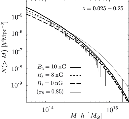
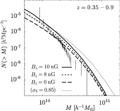
Figure 1: The integrated number counts of X-ray galaxy clusters. The left panel shows the number count for the low redshift bin $z=0.025-0.25$, while the right panels shows that for the high redshift bins $z=0.35-0.90$. In both panels, the solid, the dashed and the dotted lines represent the number counts for the case of $B_{\lambda}=10~{}$nG, $B_{\lambda}=8~{}$nG and $B_{\lambda}=0~{}$nG, respectively. We also plot the results of Chandra in Vikhlinin et al. (2009). For comparison, we put the number counts for the $B_{\lambda}=0~{}$nG case with $\sigma_{8}=0.85$ as the thin solid line.

4 S-Z number counts

The S-Z effect is caused by the scattering of CMB photons with electrons in hot gas in galaxy clusters. The change of the CMB intensity with the frequency $\nu$ by the S-Z effect is expressed, in the R-J limit, as (Sunyaev & Zeldovich, 1972; Birkinshaw, 1999)

$$I_{\nu}(\theta)=2\nu^{2}T_{\rm CMB}g(x)y(\theta),$$ (18)

where $T_{CMB}$ is the CMB temperature and $g(x)$ is the S-Z effect spectral shape given by $g(x)=x^{2}e^{x}(x/\tanh(x/2)-4)/(e^{x}-1)^{2}$ with $x=2\pi\nu/T_{\rm CMB}$. The Compton $y$-parameter is given by the integral of the electron gas pressure along the line of sight at $\theta$

$$y(\theta)=\int dl~{}f_{g}{T_{e}\over\mu_{e}m_{e}}n_{e}\sigma_{T},$$ (19)

where $T_{e}$ is the electron gas temperature, $n_{e}$ is the electron density, $\sigma_{\rm T}$ is the Thomson scattering cross-section, $m_{e}$ is the electron mass, $\mu_{e}$ is the mean mass per electron $\mu_{e}=1.143$ and $f_{g}$ is a gas fraction in a galaxy cluster which we set $f_{g}=0.12$ (Mohr et al., 1999). In the S-Z cluster survey, it is assumed that the S-Z cluster is a point like source within the telescope beam. Therefore, we consider the total flux density from a cluster at redshift $z$ by integrating the cluster surface,

$$S_{\nu}=2\nu^{2}T_{\rm CMB}g(x){Y\over D_{a}^{2}},$$ (20)

where $D_{a}$ is the angular diameter distance to the cluster at $z$ and $Y$ is the integrated $y$-parameter over the cluster surface,

$$Y=\int d\Omega~{}y(\theta).$$ (21)

In order to calculate Eq. (21), we need the electron density profile in a galaxy cluster. We take the assumption that the electron density profile is isothermal $\beta$-profile (Cavaliere & Fusco-Femiano, 1976),

$$n_{e}(r)=\left\{\begin{array}[]{cc}n_{0}\left(1+{r^{2}\over R_{\rm c}^{2}}\right)^{-{3\beta\over 2}}&r<R_{\rm v}\\ 0&r\geq R_{\rm v}\end{array}\right.$$ (22)

where $R_{c}$ is the core radius of galaxy cluster which is related to the virial radius $R_{\rm v}$ with the parameter $s(z)$ as $R_{c}=R_{\rm v}/s(z)$. Following Komatsu & Seljak (2002), we set

$$s(z)\approx\frac{10}{1+z}\left[\frac{M}{M_{*}(0)}\right]^{-0.2},$$ (23)

where $M_{*}(0)$ is a solution to $\sigma(M)=\delta_{c}$ at the redshift $z=0$, where $\delta_{c}$ is the critical density contrast for collapsing.

Taking the assumption that the galaxy clusters are spherical and in the hydrodynamical equilibrium, we can relate the virial mass $M_{\rm v}$ with the virial radius,

$$M_{\rm v}={4\pi\over 3}\rho_{\rm M}(z)\Delta_{\rm v}(z)R_{\rm v}^{3},$$ (24)

where $\Delta_{\rm v}(z)$ is the overdensity contrast for virialization (Nakamura & Suto, 1997).

We introduce the electron density weighted average temperature $\langle T_{\rm e}\rangle_{n}$, which is defined by $\langle T_{\rm e}\rangle_{n}\equiv\int dln_{e}T_{e}/\int dln_{e}$. Battye & Weller (2003) has obtained $\langle T_{\rm e}\rangle_{n}$ under the isothermal assumption in the $\lambda$CDM model,

$$\langle T_{\rm e}\rangle_{n}=T_{\star}~{}{\rm keV}\left[{M_{\rm vir}\over 10^{15}h^{-1}M_{\odot}}\right]^{2/3}\left[\Delta_{\rm c}(z){H(z)^{2}\over H_{0}^{2}}\right]^{1/3}\left[1-2{(1-\Omega_{m}(z))\over\Delta_{\rm c}(z)}\right],$$ (25)

where $T_{\star}$ is the temperature normalization factor and they adopt $T_{\star}=1.6$ for agreement with numerical simulation works in Bryan & Norman (1998) and Pierpaoli et al. (2001).

Using the $\beta$-profile assumption with the electron density weighted average temperature given by in Eq. (25), we can write the $y$-parameter as

$$y(\theta)={\langle T_{e}\rangle_{n}\over m_{\rm e}}{f_{\rm gas}M_{\rm vir}\over\mu_{e}m_{\rm p}}\sigma_{\rm T}\zeta(\theta),$$ (26)

where $\zeta(\theta)$ is the projected profile of the electron density,

$$\zeta(\theta)=\left(1+{\theta^{2}\over\theta_{c}^{2}}\right)^{-{1\over 2}}{\tan^{-1}\left[\left({s^{2}-\theta^{2}/\theta_{c}^{2}\over 1+\theta^{2}/\theta_{c}^{2}}\right)^{1/2}\right]\over{\tan^{-1}s}},$$ (27)

In actual observations, the finite beam size of telescopes causes the beam-smearing effect. This effect can be accounted by modifying Eq. (21) to (Bartlett, 2000)

$$Y=\int d\Omega~{}y(\theta)B(\theta).$$ (28)

Here we assume that the beam profile is described in a Gaussian form $B(\theta)=\exp[-\theta^{2}/(2\sigma_{b}^{2})]$ with $\sigma_{b}=\theta_{\rm FWHM}/\sqrt{8\ln 2}$ where $\theta_{\rm FWHM}$ is the full-width-half-maximum (FWHM).

The parameter $Y$ depends on the mass and the redshift of galaxy clusters. Therefore, giving the flux limit $S_{\rm lim}$ of the observation, we can obtain the limit mass of galaxy clusters $M_{L}$ at each redshift. We show $M_{L}$ for Planck and SPT in Fig. 2. We present the parameter value for each observation in Table 1. Planck will cover the full sky and the Planck sensitivity is 14 mJy at 100 GHz. SPT covers $\Delta\Omega=4000$ degree square and the SPT sensitivity is 0.8 mJy at 150 GHz. SPT has a better sensitivity than Planck. As a result, $M_{L}$ for SPT is lower than for Planck.

The combination between the S-Z galaxy cluster survey and the follow-up optical observation enables us to obtain the cluster number count for redshift bins. In Fig. 3, we show the number count of galaxy clusters with mass higher than the limiting mass shown in Fig. 2,

$$\Delta N(z)={dn\over dz}\Delta z=\Delta\Omega\int_{M_{L}}dM{dV\over dzd\Omega}{dn\over dM}{\Delta z}.$$ (29)

In both panels of Fig. 3, we set $\Delta z=0.1$ and the primordial magnetic field spectral index $n=-2.8$.

Fig. 3 shows that the predicted number counts of Planck and SPT are almost same in low redshifts. This is because, although $\it Planck$ has less sensitive to small galaxy clusters than SPT, $\it Planck$’s full sky survey area increases the number of the observed galaxy clusters, and vice versa. However, in high redshift, since the number of large-mass clusters rapidly decreases, the number count for $\it Planck$ become much lower than for SPT.

Primordial magnetic fields generate additional density fluctuations in small scales and bring the early structure formation. Therefore, the difference from $\Lambda$CDM cosmology due to the existence of primordial magnetic fields is emphasized in the SPT observation, especially in high redshifts. Even the primordial magnetic fields with $B_{\lambda}=6~{}$nG amplifies the number count in high redshifts by 50 % for the SPT sensitivity, while, for Planck, such primordial magnetic fields cannot bring a significant amplification.

For reference, we put the number counts for the $B_{\lambda}=0~{}$nG case with $\sigma_{8}=0.85$ as the thin solid line in both panels in Fig. 3. Although $\sigma_{8}$ in the case of $B_{\lambda}=10~{}$nG corresponds to $0.8$, the power spectrum in the case of $B_{\lambda}=10~{}$nG has larger amplitudes in high $k$s than in the case of $\sigma_{8}=0.85$ without primordial magnetic fields. This results in the fact the number of galaxy clusters with small mass is larger in the case of $B_{\lambda}=10~{}$nG than in the case of $\sigma_{8}=0.85$. Therefore, the number counts for $B_{\lambda}=10~{}$nG exceed the ones for $\sigma_{8}=0.85$ in the low redshifts where both Planck and SPT are sensitive to low mass clusters as shown Fig. 2. In particular, the number counts of SPT for $B_{\lambda}=10$nG is almost same as for $\sigma_{8}=0.85$ even in high redshifts, because SPT has small limiting mass.

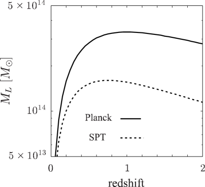
Figure 2: The limiting mass for each redshift. The solid line is for Planck and the dashed line is for SPT. The each experimental parameters are in Table. 1.

	$S_{\rm lim}$	$\nu~{}[{\rm GHz}]$	$\theta_{\rm fwhm}$	$\Delta\Omega~{}[{\rm deg}^{2}]$
Planck	$14~{}$mJy	$100$	$9.^{\prime}$	full sky
SPT	$0.8~{}$mJy	$150$	$1.^{\prime}$	$4000$

Table 1: The experimental parameters for S-Z surveys.

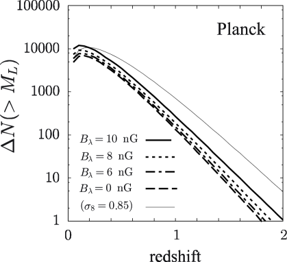
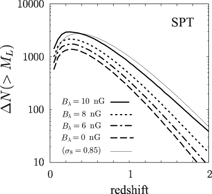
Figure 3: The integrated number counts of S-Z galaxy clusters. The left panel is for Planck, and the right panels is for SPT. In both panels, the solid, the dashed, the dashed-dotted and the dotted lines represent the number counts for the case of $B_{\lambda}=10~{}$nG, $B_{\lambda}=8~{}$nG, $B_{\lambda}=6~{}$nG and $B_{\lambda}=0~{}$nG, respectively. For comparison, we put the number counts for the $B_{\lambda}=0~{}$nG case with $\sigma_{8}=0.85$ as the thin solid line.

5 conclusion

In this paper, we have studied the effect of primordial magnetic fields on the galaxy survey by X-ray and S-Z observation. The primordial magnetic fields generate additional density fluctuations which has a blue power spectrum. Therefore, the number of galaxy clusters, especially small ones, is enhanced. X-ray and S-Z survey can directly observe this enhancement. Nano-Gauss primordial magnetic fields bring observable enhancement of the number count by the order of factors.

For X-ray cluster surveys, we have used Chandra’s result to put a constraint on the amplitude of primordial magnetic fields. We have found that Chandra’s result rules out the existence of primordial magnetic fields with $B_{\lambda}\gtrsim 10~{}$nG at roughly one-sigma level.

S-Z cluster surveys also have a sensitivity to constrain primordial magnetic fields. Especially the observation like SPT which has small limiting mass with 1 arcmin angular resolution is a good probe of primordial magnetic fields. We have found that the combination with high redshift optical surveys has the potential to put the constraint on the fields of nano Gauss order.

In this paper, we consider only primordial magnetic fields with $n=-2.8$. The power spectrum of the density fluctuations generated by primordial magnetic fields has a dependence on the spectral index of the primordial magnetic fields. The large spectral index induces the large amplification of the density fluctuations on small scales and increases the mass function for small-mass clusters. For example, $B_{\lambda}=4~{}$nG and $n=-2.5$ amplifies the number count in high redshifts by 50 % for the SPT sensitivity, comparing with the number count without primordial magnetic fields. This amplification is same as in the case of $B_{\lambda}=6~{}$nG with $n=-2.5$. Therefore, SPT has the potential to put the strong constraint on the primordial magnetic fields with large $n$.

In our calculation, we ignore the effect of primordial magnetic field on the structure of a halo. However, in order to obtain a highly accurate constraint on primordial magnetic fields, it is necessary to study the modification on the electron density profile and the relation between the X-ray temperature and the cluster mass by primordial magnetic fields. For example, Zhang (2004) and Gopal & Roychowdhury (2010) pointed out that magnetic fields with several $\mu$Gauss in a halo modify the electron density profile and this modification change the S-Z effect signal. The adiabatic contraction in the halo formation easily amplifies the order of nano Gauss of primordial magnetic field strength to the order of $\mu$ Gauss. Taking into account such effects, we will study the constraint on primordial magnetic fields through X-ray and S-Z surveys in the future.

References

- Bartlett (2000) Bartlett J. G., 2000, ArXiv Astrophysics e-prints
- Battye & Weller (2003) Battye R. A., Weller J., 2003, Phys.Rev.D, 68, 083506
- Bernet et al. (2008) Bernet M. L., Miniati F., Lilly S. J., Kronberg P. P., Dessauges-Zavadsky M., 2008, Nature, 454, 302
- Birkinshaw (1999) Birkinshaw M., 1999, Phys.Rep., 310, 97
- Brandenburg & Subramanian (2005) Brandenburg A., Subramanian K., 2005, Phys. Rep., 417, 1
- Bryan & Norman (1998) Bryan G. L., Norman M. L., 1998, Ap.J., 495, 80
- Cavaliere & Fusco-Femiano (1976) Cavaliere A., Fusco-Femiano R., 1976, Astron.Ap., 49, 137
- Giovannini (2004) Giovannini M., 2004, International Journal of Modern Physics D, 13, 391
- Giovannini (2008) Giovannini M., 2008, in M. Gasperini & J. Maharana ed., String Theory and Fundamental Interactions Vol. 737 of Lecture Notes in Physics, Berlin Springer Verlag, Magnetic Fields, Strings and Cosmology. pp 863–+
- Gopal & Roychowdhury (2010) Gopal R., Roychowdhury S., 2010, Journal of Cosmology and Astro-Particle Physics, 6, 11
- Gopal & Sethi (2003) Gopal R., Sethi S. K., 2003, Journal of Astrophysics and Astronomy, 24, 51
- Ichiki et al. (2006) Ichiki K., Takahashi K., Ohno H., Hanayama H., Sugiyama N., 2006, Science, 311, 827
- Jedamzik et al. (1998) Jedamzik K., Katalinić V., Olinto A. V., 1998, Phys.Rev.D, 57, 3264
- Kim et al. (1996) Kim E.-J., Olinto A. V., Rosner R., 1996, ApJ, 468, 28
- Komatsu & Seljak (2002) Komatsu E., Seljak U., 2002, MNRAS, 336, 1256
- Kronberg et al. (2008) Kronberg P. P., Bernet M. L., Miniati F., Lilly S. J., Short M. B., Higdon D. M., 2008, ApJ, 676, 70
- Kulsrud et al. (1997) Kulsrud R., Cowley S. C., Gruzinov A. V., Sudan R. N., 1997, Phys. Rep., 283, 213
- Mack et al. (2002) Mack A., Kahniashvili T., Kosowsky A., 2002, Phys.Rev.D, 65, 123004
- Mantz et al. (2010) Mantz A., Allen S. W., Rapetti D., Ebeling H., 2010, MNRAS, pp 1029–+
- Mohr et al. (1999) Mohr J. J., Mathiesen B., Evrard A. E., 1999, Ap.J., 517, 627
- Nakamura & Suto (1997) Nakamura T. T., Suto Y., 1997, Progress of Theoretical Physics, 97, 49
- Pierpaoli et al. (2001) Pierpaoli E., Scott D., White M., 2001, MNRAS, 325, 77
- Schleicher et al. (2009) Schleicher D. R. G., Banerjee R., Klessen R. S., 2009, Ap.j, 692, 236
- Sethi & Subramanian (2005) Sethi S. K., Subramanian K., 2005, MNRAS, 356, 778
- Sethi & Subramanian (2009) Sethi S. K., Subramanian K., 2009, Journal of Cosmology and Astro-Particle Physics, 11, 21
- Shaw & Lewis (2010) Shaw J. R., Lewis A., 2010, ArXiv e-prints
- Subramanian & Barrow (1998) Subramanian K., Barrow J. D., 1998, Phys.Rev.D, 58, 083502
- Sunyaev & Zeldovich (1972) Sunyaev R. A., Zeldovich Y. B., 1972, Comments on Astrophysics and Space Physics, 4, 173
- Takahashi et al. (2005) Takahashi K., Ichiki K., Ohno H., Hanayama H., 2005, Physical Review Letters, 95, 121301
- Tashiro & Sugiyama (2006a) Tashiro H., Sugiyama N., 2006a, MNRAS, 368, 965
- Tashiro & Sugiyama (2006b) Tashiro H., Sugiyama N., 2006b, MNRAS, 372, 1060
- Tashiro & Sugiyama (2011) Tashiro H., Sugiyama N., 2011, MNRAS, 411, 1284
- Tinker et al. (2008) Tinker J., Kravtsov A. V., Klypin A., Abazajian K., Warren M., Yepes G., Gottlöber S., Holz D. E., 2008, Ap.J., 688, 709
- Vikhlinin et al. (2009) Vikhlinin A., Burenin R. A., Ebeling H., Forman W. R., Hornstrup A., Jones C., Kravtsov A. V., Murray S. S., Nagai D., Quintana H., Voevodkin A., 2009, Ap.J., 692, 1033
- Vikhlinin et al. (2009) Vikhlinin A., Kravtsov A. V., Burenin R. A., Ebeling H., Forman W. R., Hornstrup A., Jones C., Murray S. S., Nagai D., Quintana H., Voevodkin A., 2009, ApJ, 692, 1060
- Wasserman (1978) Wasserman I., 1978, ApJ, 224, 337
- Widrow (2002) Widrow L. M., 2002, Reviews of Modern Physics, 74, 775
- Zhang (2004) Zhang P., 2004, MNRAS, 348, 1348