Considering anomalous dimensions in AdS/QCD models

Abstract

We discuss an AdS / QCD model that consider anomalous dimensions. The effect of this kind of dimensions is considered as a mass term that depend on holographical coordenate for duals modes in bulk.

I Introduction

According common AdS / CFT dictionary, operators in a field theory has dimensions related to conformal dimension of dual modes that are propagating inside the bulk, but in general these dimensions are disregarded. A property of anomalous dimensions is his scale dependence, and this can be considered in AdS side using a mass term that depend on holographical coordinate for dual modes related to operator with anomalous dimensions. In this talk we discuss this alternative in AdS / QCD models that consider explicitly effect of chiral symmetry breaking in the lagrangian Erlich:2005qh ; Da Rold:2005zs

One kind of such models, known as hard wall, allows to break chiral symmetry both spontaneously and explicitly in an independent way, but the hadronic spectra calculated in this case turns out to be not good. This situation can be improved by the introduction a dilaton field, which in many articles is considered quadratic in the holographical coordinate z Karch:2006pv . The obtained spectra has Regge behavior, but unfortunately it is not possible now to break chiral symmetry explicitly and spontaneously Colangelo:2008us .

The satisfactory implementation of chiral symmetry breaking, without sacrificing the hadronic spectra, is a problem that has attracted much interest lately. Examples of these kind of efforts can be found in Zuo:2009dz ; Gherghetta:2009ac ; Kwee:2007nq ; Sui:2009xe ; Zhang:2010tk . In this talk we show a different alternative, since we consider that the mass for modes propagating inside the bulk can present a dependence on the holographical coordinate z Vega:2010ne , which could be due to the fact that operators associated to these modes might have an anomalous dimension Cherman:2008eh .

It is possible to find references to z dependent masses in the literature Cherman:2008eh , where the authors suggest that the anomalous dimension of operators can be translated into z dependent masses for dual modes of these operators. This idea was used successfully in Vega:2008te , where an holographic model without explicit chiral symmetry breaking was considered, and which can reproduce the hadronic spectrum for spin 1/2 and 3/2 baryons with with an arbitrary number of constituents. As is known for spin 1/2 case, a dilaton field can not improve hard wall models, because this field is factorized from the equation that gives us the spectra Kirsch:2006he ; Vega:2008te . Other work related to mass varying in the bulk can be found in papers such as Forkel:2007cm ; Forkel:2007zz ; dePaula:2009za ; deTeramond:2008ht .

In this talk we consider an AdS / QCD model that takes into account effects of chiral symmetry breaking, with z dependent scalar mode masses. Thus we show that it is possible to build a model that incorporates both spontaneous and explicit chiral symmetry breaking, and which includes variable masses. In the model presented, to certain set of parameter, we obtain that lighter scalar meson has a mass lower that of the Pion, contradicting some properties of QCD Weingarten:1983uj ; Witten:1983ut , but this problem, fortunately no show for all the cases, so the model discussed here can be considered as a complementary alternative treatment for this problem, different to the effort developed in Gherghetta:2009ac ; Kwee:2007nq ; Sui:2009xe , where the authors try to improve soft wall models by deforming the dilaton and/or the metrics.

The work consists of the following parts. Section II is a brief description of the model, where we write down the equations that describe the vev and the scalar, vector and axial vector mesons in the AdS side. In III we obtain a variable mass for the scalar modes. In section IV we discuss how to fix the parameters involved in this model, in order to obtain in section V the spectra with the parameters of the previous section. Finally, section VI is dedicated to expose the conclusions of this work.

II Model

Table 1: Field content and dictionary of the model.

	4D : O(x)			5D : $\Phi(x,z)$			p			$\Delta$			$m_{5}^{2}R^{2}$
	$\overline{q}_{L}\gamma^{\mu}t^{a}q_{L}$			$A_{L\mu}^{a}$			1			3			0
	$\overline{q}_{R}\gamma^{\mu}t^{a}q_{R}$			$A_{R\mu}^{a}$			1			3			0
	$\overline{q}_{R}^{\alpha}q_{L}^{\beta}$			$\frac{1}{z}X$			0			$3+\delta$			$m_{5}^{2}(z)R^{2}$

First, in a brief way we like to remember that dimensions of operator in a field theory involved in the AdS / CFT correspondence are related with conformal dimension of dual modes in AdS side. In general, operator dimensions in a theory like QCD has anomalous dimensions that run with energy scale, and for other side, conformal dimensions for AdS modes depend on mass of this modes. If we consider other part of adS / CFT dictionary that say us the holographical coordenate z is related with energy, the relationship between dimension for operators in the field theory and conformal dimension for gravity modes tell us the mass for modes propagating inside the bulk must be z dependent.

We consider the most usual version of soft wall AdS / QCD models, with the notation used in Gherghetta:2009ac , which takes into account an 5d AdS background defined by

$$ds^{2}=\frac{R^{2}}{z^{2}}(\eta_{\mu\nu}dx^{\mu}dx^{\nu}+dz^{2}),$$ (1)

where R is the AdS radius, the Minkowsky metric is $\eta_{\mu\nu}=diag(-1,+1,+1,+1)$ and z is a holographical coordinate defined in $0\leq z<\infty$. Here we consider a usual quadratic dilaton

$$\phi(z)=\lambda^{2}z^{2}.$$ (2)

To describe chiral symmetry breaking in the mesonic sector in the 5d AdS side, the action considers $SU(2)_{L}\times SU(2)_{R}$ gauge fields and a scalar field X. Such action is given by

$$S_{5}=-\int d^{5}x\sqrt{-g}e^{-\phi(z)}Tr\biggl{[}|DX|^{2}+m_{X}^{2}(z)|X|^{2}$$

$$+\frac{1}{4g_{5}^{2}}(F_{L}^{2}+F_{R}^{2})\biggr{]}.$$ (3)

This action shows explicitly that the scalar modes masses are z dependent, which is the feature that distinguishes this model from other AdS / QCD models with chiral symmetry breaking.

In Table I the fields included in model are shown and also his relationship with modes propagating in the bulk, according to AdS / CFT dictionary. Notice that the operator $q\overline{q}$ has an anomalous dimension ($\delta$), which in turn produces a mass that depends on z for the modes dual to this operator, in agreement with Cherman:2008eh ; Vega:2008te .

Starting from (3), the equations that describe the vev and the scalar, vector and axial vector mesons are

$$-z^{2}\partial_{z}^{2}v(z)+z(3+2\lambda^{2}z^{2})\partial_{z}v(z)+m_{X}^{2}(z)R^{2}v(z)=0.$$ (4)

$$-\partial_{z}^{2}S_{n}(z)+\biggl{(}\frac{3}{z}+2\lambda^{2}z\biggr{)}\partial_{z}S_{n}(z)+\frac{m_{X}^{2}(z)R^{2}}{z^{2}}S_{n}(z)=M_{S}^{2}S_{n}(z),$$ (5)

$$-\partial_{z}^{2}V_{n}(z)+\biggl{(}\frac{1}{z}+2\lambda^{2}z\biggr{)}\partial_{z}V_{n}(z)=M_{V}^{2}V_{n}(z),$$ (6)

$$-\partial_{z}^{2}A_{n}(z)+\biggl{(}\frac{1}{z}+2\lambda^{2}z\biggr{)}\partial_{z}A_{n}(z)+\frac{R^{2}g_{5}^{2}v^{2}(z)}{z^{2}}A_{n}(z)=M_{A}^{2}A_{n}(z).$$ (7)

Before discussing the phenomenology of this model, it is necessary to know the precise form of $m_{X}^{2}(z)$, something we will now consider.

III Obtaining an expression for $m_{X}^{2}(z)$

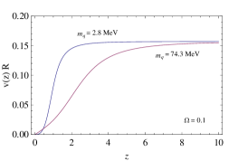
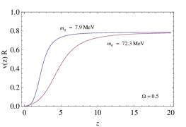
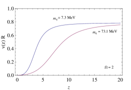
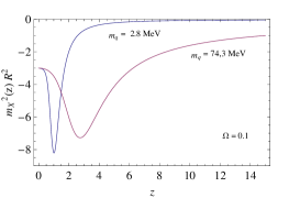
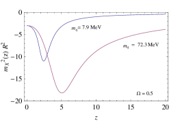
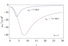
Figure 1: The upper graph shows $v(z)R$, while in the lower graph the scalar modes masses as functions of z are given. All plots have been obtained with $\lambda=0.4GeV$, and $\Omega$ values used appear in each plot.

The mass for scalar modes in the bulk, $m_{X}^{2}(z)$, is obtained starting from (4), although knowing first the function $v(z)$. The behavior of this function is known in two limits.

First we consider the usual limit $z\rightarrow 0$, according to which

$$v(z\rightarrow 0)=\alpha z+\beta z^{3},$$ (8)

where the $\alpha$ and $\beta$ coefficient are associated with the quark mass and chiral condensate respectively.

The other limit in which we know the behavior of $v(z)$ is when $z\rightarrow\infty$, and therefore we require that (7) gives a Regge-like in this limit. In order to expose this clearly, we change (7) using

$$A_{n}(z)=\exp\biggl{(}\frac{1}{2}\int\biggl{(}\frac{1}{z}+2\lambda^{2}z\biggr{)}dz\biggr{)}a_{n}(z).$$ (9)

This transformation converts our equation into a Schrödinger like equation, with a potential

$$V_{A}(z)=\frac{3}{4z^{2}}+\lambda^{4}z^{2}+\frac{R^{2}g_{5}^{2}v^{2}(z)}{z^{2}}.$$ (10)

As is well known, soft wall models must reproduce spectra with Regge behavior when $z\rightarrow\infty$, so the potential in this limit must look like

$$V(z)=a+bz^{2}+\frac{c}{z^{2}},$$ (11)

and therefore $v(z\rightarrow\infty)$ can be: constant, linear or quadratic in z. In this work we only consider the first possibility, leaving for future work a more general discussion that considers all cases.

Knowing the behavior of $v(z)$ both for $z\rightarrow 0$ as in $z\rightarrow\infty$, we choose an ansatz capable to reproduce both limits,

$$v(z)=\frac{\Omega}{R}\arctan(Az+Bz^{3}).$$ (12)

Using this form for $v(z)$ in (4) allows us to get an expression for $m_{X}^{2}(z)$. Both $v(z)$ and $m_{X}(z)$ are shown in FIG 1 to different values for $\Omega$, where this is an arbitrary parameter and parameters A and B are related to quarks mass and chiral condensate and his values are fixed according to next section.

IV Parameter setting

The first parameter that we fix is $\lambda$, using data from the spectrum. Specifically we consider a specific value for the Regge slope, which in this kind of models with quadratic dilaton is $4\lambda^{2}$. In Gherghetta:2009ac a Regge slope is fixed through radial excitations with $n\geq 3$, but in our case, since the model has Regge behavior in the vector meson sector, we use a value fixed by the lightest vector meson, so finally we choose $\lambda=0.400GeV$ that allows us to obtain correct value masses for vector mesons.

Table 2: Scalar meson spectra in MeV. Values for $\Omega$ are: (a) $\Omega=0.1$, (b) $\Omega=0.5$ y (c) $\Omega=2$. As you can see in FIG 2, for each $\Omega$ there are two possible values for $m_{q}$. All masses are in MeV.

n	$f_{0}(Exp)$	$f_{0}(a)$	$f_{0}(a)$	$f_{0}(b)$	$f_{0}(b)$	$f_{0}(c)$	$f_{0}(c)$	$f_{0}(Ref.[6])$
		$m_{q}=2.8$	$m_{q}=74.3$	$m_{q}=7.9$	$m_{q}=72.3$	$m_{q}=7.3$	$m_{q}=73.1$
0	$550^{+250}_{-150}$	162	711	130	506	84	466	799
1	$980\pm 10$	1151	1179	1130	1036	1020	932	1184
2	$1350\pm 150$	1416	1444	1411	1357	1354	1253	1466
3	$1505\pm 6$	1635	1659	1632	1597	1595	1511	1699
4	$1724\pm 7$	1823	1846	1823	1799	1796	1729	1903
5	$1992\pm 16$	1999	2014	1995	1976	1974	1918	2087
6	$2103\pm 8$	2156	2169	2152	2137	2135	2089	2257
7	$2314\pm 25$	2303	2314	2299	2286	2284	2244	2414

The remaining parameters can be fixed using (12), the expression chosen to describe the vev, which has the limits

$$v(z\rightarrow 0)=\frac{\Omega}{R}Az+\frac{\Omega}{R}\biggl{(}-\frac{A^{3}}{3}+B\biggr{)}z^{3}+O(z^{5}),$$ (13)

$$v(z\rightarrow\infty)=\frac{\Omega\pi}{2R}+O(z^{-3}).$$ (14)

Comparing (13) with the value established in the AdS / CFT dictionary, with the notation used in Gherghetta:2009ac

$$v(z\rightarrow 0)=\frac{m_{q}\zeta}{R}z+\frac{\sigma}{R\zeta}z^{3},$$ (15)

The parameter $\zeta$ was introduced in Cherman:2008eh to get the right normalization, and his value is $\zeta=\sqrt{3}/(2\pi)$. With this, the A and B parameters are given by

$$A=\frac{\sqrt{3}}{2\pi\Omega}m_{q}$$ (16)

and

$$B=\frac{2\pi}{\sqrt{3}\Omega}\sigma+\frac{3\sqrt{3}}{8\pi^{3}\Omega^{3}}m^{3}_{q},$$ (17)

where $m_{q}$ is the quark mass and $\sigma$ is the chiral condensate.

In order to finish the model description, it is necessary to specify the values for $m_{q}$ and $\sigma$, which are related by the GOR $m^{2}_{\pi}f^{2}_{\pi}=2m_{q}\sigma$, and therefore we need to fix only one of them. In this case we use $m_{\pi}=140MeV$ and $f_{\pi}=92MeV$, and we fix the quark mass using

$$f^{2}_{\pi}=-\frac{1}{g^{2}_{5}}\lim_{\epsilon\rightarrow 0}\frac{\partial_{z}A_{0}(0,z)}{z}|_{z=\epsilon},$$ (18)

where $A_{0}(0,z)$ is solution of (7), with $M^{2}_{A}=0$, and the boundary conditions used are $A_{0}(0,0)=1$ and $\partial_{z}A_{0}(0,z\rightarrow\infty)=0$.

As you can see in (7), $A_{0}(0,z)$ equation as a term that depend on $m_{q}$, so using (18) we get $f_{\pi}(m_{q})$. This appear in FIG 2, and this show us for each $\Omega$ value, we have two possible quark masses. For $\Omega=0.1$ we found $m_{q}=2.8MeV$ and $m_{q}=74.3MeV$; for $\Omega=0.5$ we get $m_{q}=7.9MeV$ and $m_{q}=72.3MeV$ and when we use $\Omega=2$ is obtained $m_{q}=7.3MeV$ and $m_{q}=73.1MeV$.

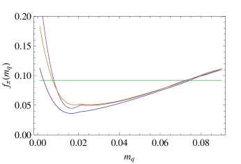
Figure 2: The plot show the pion decay constant as $m_{q}$ function according to (18). The horizontal line correspond to $f_{\pi}=92MeV$.

V Mesonic spectrum

Having fixed the parameters of the model, we can calculate masses for some mesons, which correspond to eigenvalues in the equations (5), (6) and (7). In this set of equations, only (6) can be solved analytically. For this reason we prefer to change all equations into Schrödinger like ones, and later solve numerically (5) and (7) using a MATHEMATICA code called schroedinger.nb Lucha:1998xc , which was adapted to our potentials.

Table 3: Vector mesons spectra in MeV.

	n			$\rho(Exp)$			$\rho(Model)$			$\rho(Ref.[6])$
	0			$775.5\pm 1$			800			475
	1			$1282\pm 37$			1131			1129
	2			$1465\pm 25$			1386			1529
	3			$1720\pm 20$			1600			1674
	4			$1909\pm 30$			1789			1884
	5			$2149\pm 17$			1960			2072
	6			$2265\pm 40$			2117			2243

Table 4: Axial vector mesons spectra in MeV. Values for $\Omega$ are: (a) $\Omega=0.1$, (b) $\Omega=0.5$ and (c) $\Omega=2$. The values for $m_{q}$ in the table. All masses are in MeV.

n	$a_{1}(Exp)$	$a_{1}(a)$	$a_{1}(a)$	$a_{1}(b)$	$a_{1}(b)$	$a_{1}(c)$	$a_{1}(c)$	$a_{1}(Ref.[6])$
		$m_{q}=2.8$	$m_{q}=74.3$	$m_{q}=7.9$	$m_{q}=72.3$	$m_{q}=7.3$	$m_{q}=73.1$
0	$1230\pm 40$	864	825	1262	888	1495	909	1185
1	$1647\pm 22$	1170	1144	1388	1231	2331	1325	1591
2	$1930^{+39}_{-70}$	1412	1394	1579	1468	2544	1649	1900
3	$2096\pm 122$	1619	1606	1755	1668	2660	1910	2101
4	$2270^{+55}_{-40}$	1803	1794	1917	1846	2770	2117	2279

VI Conclusions

The possibility of incorporating chiral symmetry breaking in soft wall models, introducing a dependence on the holographical coordinate in the mass for models propagating inside the bulk, was studied. This idea could be considered as a complement to other mechanisms that try to solve this problem introducing changes in the dilaton field, changes in the metric, or introducing a cubic or quartic term for scalars in the action Gherghetta:2009ac ; Kwee:2007nq ; Sui:2009xe ; Zhang:2010tk .

The model considered here uses a usual quadratic dilaton and a AdS metric, and considers an expression for $v(z)$ that it is able to reproduce the expected behavior in the UV and IR limits. For certain choice of parameters is obtained that the mass of the lightest scalar meson is less than the mass of the Pion, contradicting a theorem well-established QCD, which fortunately for the model is not so in all cases, then it is possible to obtain mesonic masses that in general are in good agreement with data.

In light of the results presented in this paper, we think that the introduction of a mass that varies with z inside the bulk can be considered as a complementary alternative in order to build AdS / QCD models that take into account effects of chiral symmetry breaking. In some cases the spectra that we get is poor, so a z dependent mass like we are presenting here clearly cannot solve all problems, but anyway we think is an interesting complementary alternative, because z dependent masses can be associated to dual modes of operators with anomalous dimensions, allowing the introduction into this kind of models of an important QCD quantity, which is usually not considered when people build AdS / QCD models.

- (1) J. Erlich, E. Katz, D. T. Son and M. A. Stephanov, Phys. Rev. Lett. 95, 261602 (2005) [arXiv:hep-ph/0501128].
- (2) L. Da Rold and A. Pomarol, Nucl. Phys. B 721, 79 (2005) [arXiv:hep-ph/0501218].
- (3) A. Karch, E. Katz, D. T. Son and M. A. Stephanov, Phys. Rev. D 74, 015005 (2006) [arXiv:hep-ph/0602229].
- (4) P. Colangelo, F. De Fazio, F. Giannuzzi, F. Jugeau and S. Nicotri, Phys. Rev. D 78, 055009 (2008) [arXiv:0807.1054 [hep-ph]].
- (5) F. Zuo, arXiv:0909.4240 [hep-ph].
- (6) T. Gherghetta, J. I. Kapusta and T. M. Kelley, Phys. Rev. D 79, 076003 (2009) [arXiv:0902.1998 [hep-ph]].
- (7) H. J. Kwee and R. F. Lebed, Phys. Rev. D 77, 115007 (2008) [arXiv:0712.1811 [hep-ph]].
- (8) Y. Q. Sui, Y. L. Wu, Z. F. Xie and Y. B. Yang, Phys. Rev. D 81, 014024 (2010) [arXiv:0909.3887 [hep-ph]].
- (9) P. Zhang, arXiv:1003.0558 [hep-ph].
- (10) A. Vega and I. Schmidt, arXiv:1005.3000 [hep-ph].
- (11) A. Cherman, T. D. Cohen and E. S. Werbos, Phys. Rev. C 79, 045203 (2009) [arXiv:0804.1096 [hep-ph]].
- (12) A. Vega and I. Schmidt, Phys. Rev. D 79, 055003 (2009) [arXiv:0811.4638 [hep-ph]].
- (13) I. Kirsch, JHEP 0609, 052 (2006) [arXiv:hep-th/0607205].
- (14) H. Forkel, M. Beyer and T. Frederico, JHEP 0707, 077 (2007) [arXiv:0705.1857 [hep-ph]].
- (15) H. Forkel, M. Beyer and T. Frederico, Int. J. Mod. Phys. E 16, 2794 (2007).
- (16) W. de Paula and T. Frederico, arXiv:0908.4282 [hep-ph].
- (17) G. F. de Teramond and S. J. Brodsky, Phys. Rev. Lett. 102, 081601 (2009) [arXiv:0809.4899 [hep-ph]].
- (18) D. Weingarten, Phys. Rev. Lett. 51, 1830 (1983).
- (19) E. Witten, Phys. Rev. Lett. 51, 2351 (1983).
- (20) W. Lucha and F. F. Schoberl, Int. J. Mod. Phys. C 10, 607 (1999) [arXiv:hep-ph/9811453].