DISTRIBUTION OF RESONANCE WIDTHS AND DYNAMICS OF CONTINUUM COUPLING

Abstract

We analyze the statistics of resonance widths in a many-body Fermi system with open decay channels. Depending on the strength of continuum coupling, such a system reveals growing deviations from the standard chi-square (Porter-Thomas) width distribution. The deviations emerge from the process of increasing interaction of intrinsic states through common decay channels; in the limit of perfect coupling this process leads to the super-radiance phase transition. The width distribution depends also on the intrinsic dynamics (chaotic vs regular). The results presented here are important for understanding the recent experimental data concerning the width distribution for neutron resonances in nuclei.

Open and marginally stable quantum systems are of great current interest in relation to numerous applications in nuclear physics of exotic nuclei, chemical reactions, condensed matter, astrophysics and quantum informatics. The general problem can be formulated as that of the signal transmission through a complicated quantum system. The complexity of theoretical description of such processes is due to the necessity of a consistent unified theory that would cover intrinsic structure, especially for many-body systems, along with cross sections of various reactions.

One of the best and historically advanced examples of the manifestation of the interplay between intrinsic dynamics and decay channels is given by low-energy neutron resonances in complex nuclei BM . The series of these well pronounced separated resonances were studied long ago porter58 ; porter60 ; porterbook and later gave rise to the “Nuclear Data Ensemble” haq82 ; sissom82 . Interpreting these resonances as quasi-stationary levels of the compound nucleus formed after the neutron capture, agreement was found with predictions of the Gaussian Orthogonal Ensemble (GOE) of random matrices. With exceedingly complicated wave functions of compound states, the statistical distribution of their components is close to Gaussian. The neutron decay implements the analysis of a specific component related to the channel “neutron in continuum plus a target nucleus in its ground state”. The neutron width is proportional to the squared amplitude of this component, and the width distribution then is $\chi^{2}_{\nu}$ with $\nu=1$ as appropriate for one channel [Porter-Thomas distribution (PTD)].

The recent experiments with improved accuracy koehler10 give evidence of significant deviations from the PTD so that the attempts to still use the $\chi^{2}_{\nu}$ distribution for the fit invariably require $\nu<1$. A non-pure set of resonances, for example, a sequence of mainly $s$-resonances contaminated by $p$-wave states, would shift the distribution to a higher number of degrees of freedom, $\nu>1$. The new result was interpreted as a consequence of an unknown non-statistical mechanism or just a breakdown of nuclear theory as was claimed in the related article in “Nature” with a title “Nuclear theory nudged” nature10 .

The goal of this letter is to point out that a correct description of unstable quantum states in a complicated many-body system naturally leads to deviations from the GOE and PTD, of the same type as observed in koehler10 . The random matrix theory was formulated for local statistics in a closed quantum system with a discrete spectrum governed by a very complicated Hermitian Hamiltonian. As such, its predictions were repeatedly checked, qualitatively and quantitatively, in systems like quantum billiards nakamura04 and their experimental embodiment in microwave cavities stockmann99 ; alt95 , and in shell-model calculations for complex atoms grib94 and nuclei big .

However, the presence of open decay channels and therefore the finite lifetime of intrinsic states unavoidably lead to new phenomena outside of the GOE framework verbaarschot85 ; SZNPA89 as it was clearly demonstrated by the first numerical simulations kleinwachter85 ; mizutori93 ; izr94 . Two interrelated effects follow from the fact that we deal with unstable rather than with strictly stationary states: the level repulsion disappears at the spacings comparable to the level widths and the growing widths undergo the redistribution with the trend to collectivization and eventually formation of super-radiant (short-lived) states along with the narrow (trapped) states SZNPA89 ; SZAP92 . The new dynamics modify the GOE predictions as well as certain features of Ericson fluctuations ericsonAP63 in the regime of overlapping resonances celardo08 . The occurrence of a super-radiant transition has been also demonstrated outside the random matrix theory framework kaplan .

A quantum many-body system coupled to open decay channels can be rigorously described by an effective non-Hermitian Hamiltonian ${\cal H}$ MW ,

$${\cal H}=H-\,\frac{i}{2}\,W.$$ (1)

Here $H$ is the Hermitian Hamiltonian of the closed system that in general includes virtual (off-shell) coupling to the continuum, while the anti-Hermitian (on-shell) part $(-i/2)W$ is constructed in terms of the amplitudes ${\bf A}=\{A^{c}_{i}\}$ coupling intrinsic states $|i\rangle$ to the open channels $c$,

$$W={\bf A}{\bf A}^{T}\quad\Rightarrow\quad W_{ij}=\sum_{c({\rm open})}^{M}A^{c}_{i}A^{c}_{j}.$$ (2)

We consider a time-reversal invariant system, when the (in general depending on running energy) amplitudes $A^{c}_{i}$ can be taken real. The factorized form of $W$ is an important property that follows from unitarity of the scattering matrix durand76 . The complex eigenvalues, ${\cal E}=E-(i/2)\Gamma$, of the Hamiltonian (1) coincide with the poles of the scattering matrix and determine the positions and the widths of the resonances in cross sections of various reactions.

The factorized matrix $W$ has $M$ non-zero eigenvalues, this number being equal to that of open channels. The matrix $H$ has dimension $N$ that in the nuclear case should include a large number of shell-model many-body states important for the dynamics in the energy range under consideration; in the region of neutron resonances, $N\sim 10^{5\div 6}\gg M$. With the trace of $W$ equal to $\eta$, the important parameter defining the dynamics is the ratio of typical “bare” widths $\eta/N$ of individual states to the energy spacings $D$. At small value of this parameter, an open channel serves as an analyzer that singles out a specific component of the exceedingly complicated intrinsic wave function. Characteristically, the resonance widths in such a system obey the PTD. With widths increasing, the system moves in the direction of the regime of overlapping resonances.

Let us consider the single-channel case, $M=1$, having in mind the $s$-wave elastic neutron resonances. With a high level density of intrinsic states at relevant energy, their local spectral statistics is close to the predictions of the GOE. Then, essentially owing to the central limit theorem, the individual components of a typical intrinsic state are Gaussian distributed uncorrelated quantities, and the neutron widths, being proportional to the absolute magnitudes of those components, display the PTD. However, the correct description of the dynamics with the continuum coupling shows the limited character of this prediction. The imaginary part (2) works similar to the collective multipole forces and creates the interaction between intrinsic states through continuum. When the coupling is weak, $\kappa=\eta/ND\ll 1$, we indeed expect to see well isolated resonances with the PTD of the widths. With growing continuum coupling (increase of energy from the threshold), the deviations become more and more pronounced. At $\kappa\sim 1$, a kind of a phase transition occurs with the sharp redistribution of widths and the segregation of a super-radiant state accumulating the lion’s share of the whole summed width, an analog of a giant resonance along the imaginary energy axis. The formal mechanism is clear from the factorized structure of $W$ that, for $M=1$, has only one non-zero eigenvalue equal to the trace of $W$. Being similar to super-radiance in optics dicke54 , this mechanism works essentially independently of the regular or chaotic nature of intrinsic dynamics.

In the case of the GOE-type dynamics of the closed system and $M=1$, the distribution of complex eigenvalues can be found analytically. The Ginibre ensemble ginibre65 of complex Gaussian matrices is not applicable since it considers the imaginary parts of the eigenvalues spread over the complex plane while physical widths are positive. The exact result, see derivation in SZNPA89 , is given by the Ullah distribution ullah69 ,

$${\cal P}(\{E_{n};\Gamma_{n}\})=C_{N}\prod_{m<n}\,\frac{|{\cal E}_{m}-{\cal E}_{n}|^{2}}{|{\cal E}_{m}-{\cal E}_{n}^{\ast}|}\prod_{n}\,\frac{1}{\sqrt{\Gamma_{n}}}\,\exp(-NF).$$ (3)

Here $C_{N}$ is a normalization constant; the pre-exponential factor describes the correlations which are reduced to the usual GOE level repulsion for stable states but for complex energies ${\cal E}_{n}$ contain the interactions with their “electrostatic images” ${\cal E}_{n}^{\ast}$. Along with the Porter-Thomas factor $\Gamma^{-1/2}$, this guarantees that the widths are positive. The “equilibrium” distribution of complex energies is determined by their “free energy”,

$$F(\{E_{n},\Gamma_{n}\})=\sum_{n}\left(\frac{E_{n}^{2}}{a^{2}}\,+\,\frac{\Gamma_{n}}{2\eta}\right)\,+\sum_{m<n}\frac{\Gamma_{m}\Gamma_{n}}{2a^{2}},$$ (4)

that includes the interaction between the widths, the last term in Eq. (4). The mean level spacing in the closed system is defined as $D=2a/N$, where $2a$ is the spectral interval of real energy. The Gaussian ensemble of the decay amplitudes is defined by the mean values $\overline{A_{n}}=0,\;\overline{A_{n}A_{m}}=(\eta/N)\delta_{mn}$. Here, a regular evolution of the widths as a function of energy of the resonance is excluded as it is usually done with the rescaling to the reduced widths; we do not discuss here the way of practical rescaling that may depend on the specific nucleus. Our main purpose here is to show that systematic deviations from the PTD occur even for the set of reduced widths, and the effects are caused by the interaction (4).

For very small widths, $\kappa\ll 1$, the width interaction is negligible, the first product in (3) reduces to the standard level repulsion, and the distribution (3) is factorized into the product of the GOE distribution of real energies and the PTD for the widths. While the usual Hermitian perturbation mixes the intrinsic wave functions and therefore makes their widths close to each other (level repulsion and width attraction), the anti-Hermitian interaction through the continuum relaxes the level repulsion but leads to the collectivization through the common decay channel and width repulsion brentano96 . In the case of $\kappa\simeq 1$, the width repulsion becomes critical, and the most probable configuration is the one where this repulsion is small because the total width is going to concentrate in a single super-radiant state SZNPA89 ; SZAP92 . With the further increase of $\kappa\gg 1$ (but for a fixed number of open channels), the broad state becomes a smooth envelope, and we return to the set of $(N-1)$ narrow resonances. Below we show the typical evolution of the width distribution studied in a large-scale numerical simulation.

In the first type of simulations, we considered $H$ as a member of the GOE Zel1 ; VWZ where the matrix elements are Gaussian random variables, $\langle H_{ij}^{2}\rangle=(1+\delta_{ij})/N$. This corresponds to the limiting case of fully chaotic intrinsic dynamics. In parallel, we also modeled $H$ by the two-body random ensemble (TBRE) for $n$ fermions distributed over $m$ single-particle states; the total number of many-body states is $N=m!/[n!(m-n)!]$; in our simulations $n=6,\;m=12,\;N=924$. The TBRE is modeled by the Hamiltonian $H=H_{0}+V$, where the mean field part $H_{0}$ is defined by single-particle energies, $\epsilon_{j}$, with a Poissonian distribution of spacings and the mean level spacing $d_{0}$. The interaction $V$ FI97 is fixed by the variance of the two-body random matrix elements, $\langle V_{1,2;3,4}^{2}\rangle=v_{0}^{2}$. While at $v_{0}=0$ we have a Poissonian spacing distribution $P(s)$ of many-body states, for $d_{0}=0$ (infinitely strong interaction, $v_{0}/d_{0}\rightarrow\infty$), $P(s)$ is close to the Wigner-Dyson distribution typical for a chaotic system. The critical interaction for the onset of strong chaos is given FI97 by $v_{cr}/d_{0}\approx 2(m-n)/N_{s}$, where $N_{s}=n(m-n)[1+(n-1)(m-n-1)/4]$ is the number of directly coupled many-body states in any row of the matrix $H_{ij}$. In our model, $v_{cr}/d_{0}\approx 1/20$.

We computed the complex eigenvalues of the effective Hamiltonian, Eq.(1), for $10^{3}$ random realizations, selecting the states at the center of the energy band where their density is almost constant.

The distribution of widths, normalized to their average value, was obtained for different strengths of continuum coupling. The numerically obtained distributions were fitted, using a standard $\chi^{2}$ test, with a $\chi^{2}_{\nu}$ distribution for $\nu$ degrees of freedom, following a common practice in nuclear data analysis. As a measure of quality of the fit we used the criterion $\chi^{2}_{r}\approx 1$, where $\chi^{2}_{r}$ is the reduced chi-square value chi . Fig. 1 shows the normalized width distribution for the GOE case with $M=1$, left panels, and $M=2$, right panels, for different coupling to the continuum, $\kappa$. The standard distributions, PTD for $M=1$, and $\chi^{2}_{\nu=2}$ for $M=2$, are valid only when the coupling to the continuum is very weak, while strong deviations from $\chi^{2}_{\nu=M}$ appear, both for large and small $\Gamma$, as we increase the coupling. In Fig. 1 we also show the best fit possible for a $\chi^{2}_{\nu}$ distribution; always the corresponding value of $\nu$ is $<M$, moreover the quality of the fit decreases as $\kappa$ increases, see discussion below. In the lowest panels in Fig. 1, the distribution of the widths is shown at the super-radiance transition, $\kappa=1$. The tail here is described by a power law, see discussion in Ref. SFT99 , meaning that no $\chi^{2}_{\nu}$ distributions would be a good fit.

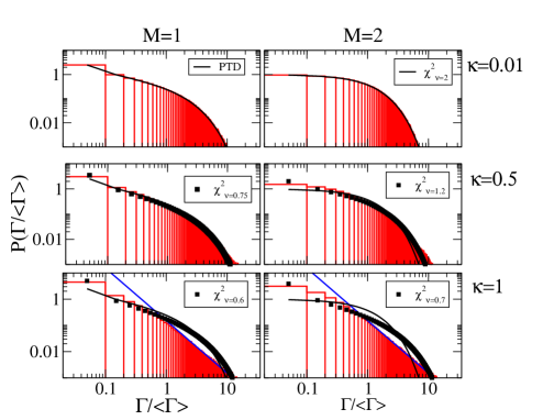
Figure 1: (Color online) Normalized distribution of the widths for one open channel, $M=1$, left panels, and for $M=2$, right panels, for the GOE intrinsic Hamiltonian and different continuum coupling strength, $\kappa$. The numerical results are shown by histograms; the expected PTD for $M=1$ and $\chi^{2}_{\nu=2}$ distribution for $M=2$ are shown by a smooth curve in all panels. With full squares we show the best fit with a $\chi^{2}_{\nu}$ distribution. In the lowest panels, a straight line shows the power law $P(\Gamma/\langle\Gamma\rangle)\propto(\Gamma/\langle\Gamma\rangle)^{-2}$. Included are the widths for the resonances in the energy interval $\pm 0.5$ for $10^{3}$ different ensemble realizations.

The dependence of the best fitted value of $\nu$ on the coupling strength is shown in Fig. 2 for $M=1$, upper panel, and for $M=2$, lower panel. Along with the data for the GOE intrinsic Hamiltonian (circles), the data for the TBRE intrinsic dynamics are shown by crosses for the case $v_{0}=d_{0}/50$ and by squares for $v_{0}=0$ (no intrinsic chaos). Regardless of intrinsic dynamics, the best value of $\nu$ steadily decreases as $\kappa$ increases. It is clear that a family of $\chi^{2}_{\nu}$ distributions is not appropriate to fit our numerical data, except for very weak continuum coupling. Indeed, the $\chi^{2}_{r}$ criterion steeply increases with the coupling strength, see insets in Fig. 2. For weak internal chaos, the departure from the $\chi^{2}_{\nu=M}$ distribution is stronger than for chaotic intrinsic dynamics, even at weak continuum coupling. The absence of intrinsic chaos and corresponding level repulsion implies a stronger sensitivity to continuum coupling.

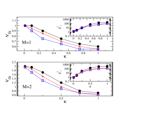
Figure 2: (Color online) The best fitted value of $\nu$ vs the coupling strength to the continuum, $\kappa$. Full circles refer to the case of GOE intrinsic Hamiltonian, crosses stand for the case of TBRE with $v_{0}=d_{0}/50$, and squares for the case of TBRE with $v_{0}=0$ (no intrinsic chaos); the number of channels is one (upper panel) and two (lower panel). The insets show the reduced chi $\chi^{2}_{r}$ as a function of $\kappa$.

When analyzing empirical neutron $s$-wave resonances one of the main difficulties is the $p$-wave contamination. In order to analyze this problem we considered the case of two non-equivalent channels, with $10\%$ of the states coupled to the additional channel by a smaller coupling strength. When another channel is included, the best fit value of $\nu$ at weak coupling is always larger than one; again this value decreases when the continuum coupling is growing. As expected, we also observed the evolution of the level spacing distribution $P(s)$ along the real axis, with disappearance of repulsion at spacings comparable with the level widths mizutori93 ; for example, at $\kappa=0.5$, $P(0)\approx 0.2$. Interesting physics related to energy-width correlations will be discussed elsewhere.

To summarize, the normalized width distributions have been analyzed for a system with $M=1$ or 2 open channels as a function of the continuum coupling strength. As this coupling increases, the best fit value of $\nu$ for a $\chi^{2}_{\nu}$ distribution decreases below $M$, in accordance to recent experimental findings koehler10 . At the same time, the fit quality becomes poor showing that the standard PTD (and in general any $\chi^{2}_{\nu}$ distribution) is applicable only for extremely narrow resonances. The low-energy neutron resonances in a heavy nucleus correspond to the very beginning of the process of width collectivization. However, already here the deviations from the (GOE$\times$PTD) factorized distribution are noticeable. These deviations are more pronounced for regular intrinsic dynamics than for chaotic intrinsic dynamics. Therefore, the interpretation of the width as a strength of the pure neutron component in the compound wave function fails due to the coupling through continuum that has to be accounted for in a proper statistical description. The phenomenon under discussion is of general nature and it may influence all processes of signal transmission through a quantum system.

We are grateful to V. Sokolov, Y. Fyodorov, and A. Volya for useful comments. N.A. thanks the NSCL and W. Mittig for hospitality and support; G.L.C. acknowledges fruitful discussions with F. Borgonovi; V.Z. acknowledges support from the NSF grant PHY-0758099. F.I. acknowledge partial support from VIEP BUAP grant EXC08-G.

References

- (1) A. Bohr and B.R. Mottelson, Nuclear Structure, Vol. 1 (World Scientific, Singapore, 1998).
- (2) C.E. Porter and R.G. Thomas, Phys. Rev. 104, 483 (1956).
- (3) C.E. Porter and N. Rosenzweig, Phys. Rev. 120, 1698 (1960).
- (4) Statistical Theories of Spectra: Fluctuations, ed. by C.E. Porter (Academic, New York, 1965).
- (5) R. Haq, A. Pandey, and O. Bohigas, Phys. Rev. Lett. 48, 1986 (1982).
- (6) D.J. Sissom, J.F. Shriner, Jr., G. Mitchell, Phys. Rev. Lett. 48, 1086 (1982).
- (7) P.E. Koehler, F. Becvar, M. Krticka, J.A. Harvey, and K.H. Guber, Phys. Rev. Lett. 105, 072502 (2010).
- (8) E.S. Reich, Nature 466, 1034 (2010).
- (9) K.Nakamura and T.Harayama, Quantum Chaos and Quantum Dots: Mesoscopic Physics and Nanotechnology (Oxford University Press, 2004).
- (10) H.-J. Stöckmann, Quantum Chaos: An Introduction (Cambridge University Press, 1999).
- (11) H. Alt, H.-D. Gräf, H.L. Harney, R. Hofferbert, H. Lengeler, A. Richter, P. Schardt, and H.A. Weidenmüller, Phys. Rev. Lett. 74, 62 (1995).
- (12) V.V. Flambaum, A.A. Gribakina, G.F. Gribakin, and M.G. Kozlov, Phys. Rev. A 50, 267 (1994).
- (13) V. Zelevinsky, B.A. Brown, N. Frazier, and M. Horoi, Phys. Rep. 276, 85 (1996).
- (14) J.J.M. Verbaarschot, H.A. Weidenmüller, and M.R. Zirnbauer, Phys. Rep. 129, 367 (1985).
- (15) V.V. Sokolov and V.G. Zelevinsky, Nucl. Phys. A504, 562 (1989).
- (16) P. Kleinwächter and I. Rotter, Phys. Rev. C 32, 1742 (1985).
- (17) S. Mizutori and V.G. Zelevinsky, Z. Phys. A346, 1 (1993).
- (18) F.M. Izrailev, D. Saher, and V.V. Sokolov, Phys. Rev. E 49, 130 (1994).
- (19) V.V. Sokolov and V.G. Zelevinsky, Ann. Phys. (N.Y.) 216, 323 (1992).
- (20) T. Ericson, Ann. Phys. 23, 390 (1963).
- (21) G.L. Celardo, F.M. Izrailev, V.G. Zelevinsky, and G.P. Berman, Phys. Lett. B 659, 170 (2008); Phys. Rev. E 76, 031119 (2007).
- (22) G. L. Celardo and L. Kaplan, Phys. Rev. B 79, 155108 (2009); E. Persson, I. Rotter, H.-J. Stöckmann, and M. Barth, Phys. Rev. Lett. 85, 2478 (2000).
- (23) C. Mahaux and H.A. Weidenmüller, Shell Model Approach to Nuclear Reactions (North Holland, Amsterdam, 1969).
- (24) L. Durand, Phys. Rev. D 14, 3174 (1976).
- (25) R.H. Dicke, Phys. Rev. 93, 99 (1954).
- (26) J. Ginibre, J. Math. Phys. 6, 3 (1965).
- (27) N. Ullah, J. Math. Phys. 10, 2099 (1969).
- (28) P. von Brentano, Phys. Rep. 264, 57 (1996).
- (29) V.V. Flambaum and F.M. Izrailev, Phys. Rev. E 56, 5144 (1997).
- (30) V. V. Sokolov and V. G. Zelevinsky, Phys. Lett. B 202, 10 (1988); Nucl. Phys. A504, 562 (1989).
- (31) J.J.M. Verbaarschot, H.A. Weidenmüller, and M.R. Zirnbauer, Phys. Rep. 129, 367 (1985).
- (32) Given a histogram with bins, the reduced chi squared is defined as , where is the observed number of events in the bin and is the expected number of events.
- (33) Y.V. Fyodorov and H.-J. Sommers, J.Math. Phys. 38, 1918 (1997); H.-J. Sommers, Y.V. Fyodorov, and M. Titov, J. Phys. A: Math. Gen. 32, L77 (1999).