Symmetry breaking: A tool to unveil the topology of chaotic scattering with three degrees of freedom

Abstract

We shall use symmetry breaking as a tool to attack the problem of identifying the topology of chaotic scatteruing with more then two degrees of freedom. specifically we discuss the structure of the homoclinic/heteroclinic tangle and the connection between the chaotic invariant set, the scattering functions and the singularities in the cross section for a class of scattering systems with one open and two closed degrees of freedom.

keywords: Chaotic Scattering, Cross sections, Classical Mechanics, Rainbow Singularities

PACS: 45.20.df 05.45.-a 45.50.-j 05.45.-a 05.45.Ac 05.45.Pq

1 Introduction

In a Hamiltonian system with two degrees of freedom the Poincare map acts on a two dimensional domain. The chaotic invariant set is represented by the well known horseshoe construction of Smale [1]. In the meantime it has been worked out quite well, how in the case of open systems (scattering systems) the properties of this chaotic set are seen in scattering functions [2, 3] and in scattering cross sections [4, 5]. The corresponding investigations become a lot more complicated when we proceed to systems with more degrees of freedom. Therefore relatively little has been done for more degrees of freedom. In the present article we present some results for one class of higher dimensional scattering systems, namely the one with one open and two closed degrees of freedom.

Our strategy to attack this higher dimensional case is based on an idea introduced to treat elliptical orbits in reduced three-body systems [6], which is actually much in the spirit of Moshinskys work in nuclear physics. We start from a system with a symmetry and a conserved quantity (in the former case the Jacobi integral). Then the three degrees of freedom system can be reduced to a continuum of systems with two degrees of freedom where the numerical value of the conserved quantity serves as parameter. We use the knowledge of the techniques for the two degree of freedom case, to treat the reduced system. Then we embed the continuum of the reduced systems into the full six-dimensional phase space to assemble the corresponding higher dimensional structures still for the symmetric case. In other words, we find the solution for the symmetric case. Finally we break the symmetry to get to the true three degrees of freedom case. Here we show that the breaking of the symmetry does not have important effects on the qualitative properties of the structure, at least as long as the symmetry breaking is weak. The argument is supported by numerical calculations.

2 The chaotic invariant set

For Hamiltonian systems with three degrees of freedom the Poincaré map acts on a four dimensional domain. The first thing to do is to describe in the domain of the four dimensional Poincaré map the higher dimensional analog of the two dimensional horseshoe we obtain, when a symmetry reduces the effective dimensionality of the system.

As representative example of the class of system we want to treat we imagine the motion of a particle in a channel with an obstacle. The empty channel is cylindrical and thereby has a rotational symmetry in the azimuth angle $\phi$. The obstacle is represented by a short range potential depending on a parameter A which describes the deviation of the obstacle from rotational symmetry. For A=0 the obstacle is symmetric in azimuth direction and the conjugate angular momentum $L$ is conserved and the rotational symmetry allows the reduction to two degrees of freedom. A natural choice for the intersection condition for the Poincare map is the choice of relative maxima of the cylindrical radius $\rho$. Every times when the particle runs through a relative maximum of $\rho$ we measure the values of $z$, $p$, $\phi$ and $L$ where $z$ and $p$ are position and conjugate momentum along the axis of the channel. The space of these four coordinates is the domain of the Poincaré map.

One possibility to proceed is to set up particular models for the channel and the potential of the obstacle and to study solutions of Hamilton’s equations of motion and to obtain the Poincare map from them. We do something simpler and more direct. We set up a model function for the Poincare map which serves as prototype example (paradigm) for the whole class of systems. We compose it from three steps:
First, half of a free flight
Second, a kick generated by the generating function

$$G(z,p^{\prime},\phi,L^{\prime})=zp^{\prime}+\phi L^{\prime}+(L_{m}-L^{\prime})(1+A\cos(\phi))V(z)$$ (1)

Here $L_{m}$ is the maximally possible value of $L$, indirectly $L_{m}$ fixes the value of the total energy $E$.
Third, again half a free flight
For the potential function $V$ appearing in Eq. 1 we take

$$V(z)=-\exp(-z^{2})$$ (2)

For $A=0$ the map becomes independent of $\phi$ and reduces to a map acting on the $z$, $p$ plane. This reduced map depends on the conserved value of $L$ as parameter.

Because the potential of Eq. 2 is purely attractive the points $z=\pm\infty$ act as outer fixed points of the map and we use their invariant manifolds to construct the horseshoe of the reduced system.

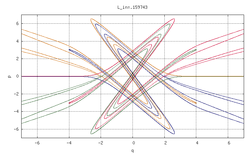
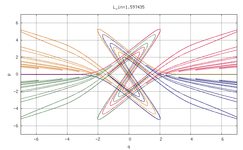
Figure 1: In this figure and in the next two figures we show the horseshoe of the reduced system for parameter value $A=0$. We show it for 6 different values of the conserved angular momentum. As can be seen, this angular momentum acts as a development parameter for the horseshoe. For values of $L_{in}$ close to zero ( as typical example the case $L_{in}=0.159749$ is seen in the upper part of the figure ) the horseshoe is complete. For larger values of $L_{in}$ it becomes incomplete. The lower part of Fig.1 shows a situation where the horseshoe has just become incomplete.

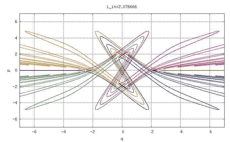
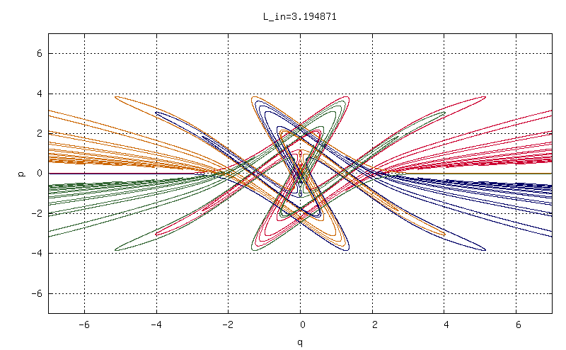
Figure 2: This figure is the continuation of Fig.1. The upper part shows the case $L_{in}=2.076666$ where the horseshoe is a little more than 2/3 developed and the lower part shows the case $L_{in}=3.194871$ where it is a little less than 2/3 developed.

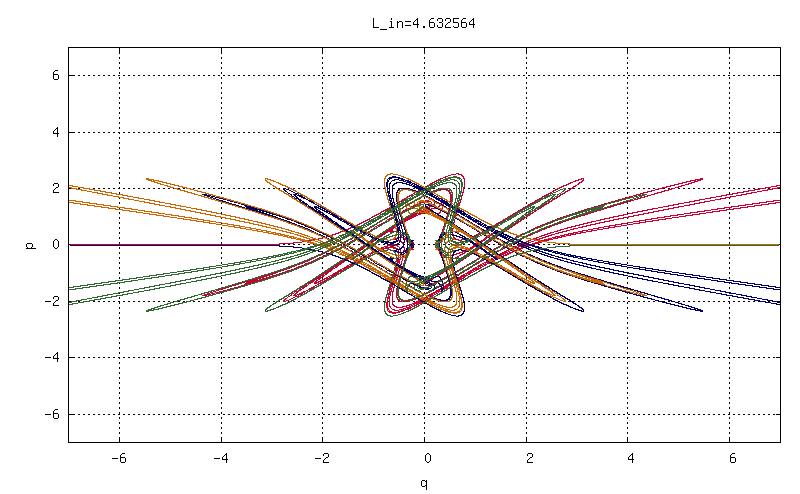
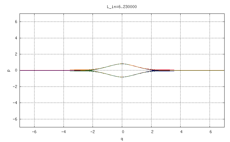
Figure 3: This figure is the continuation of Figs.1 and 2. The upper part shows the case $L_{in}=4.632564$ where the horseshoe is developed to the degree of almost one third. The lower part shows a case where $L_{in}$ comes close to its maximally allowed value $L_{m}$ at which the horseshoe development degree goes to zero, i.e. where the horseshoe collapses to a parabolic line.

Figs. 1, 2, 3 shows the result for various values of $L$. As function of $L$ we see the standard development scenario of a ternary symmetric horseshoe. When $L$ goes from zero to approximately 5.5 the relative development stage of the homoclinic/heteroclinic tangle shown in Figs. 1, 2, 3 goes from zero to one, for more details on the introduction of a quantitative development parameter for a ternary symmetric horseshoe see [3].

The transition to the higher dimensional structures, still for the symmetric case, is now easy. The angular momentum $L$ which serves as parameter in the two dimensional map is a coordinate of the domain of the four dimensional map. Therefore we just form the pile of the whole continuum of two dimensional cases. This three dimensional structure is an intermediate step for the final four dimensional structure. To include the final coordinate $\phi$ is completely trivial. We just form the Cartesian product of the three dimensional intermediate step with a circle representing the coordinate $\phi$. The result is the final homoclinic/heteroclinic tangle in the four dimensional map. In this process the outer fixed point at $z=\pm\infty$ of the two dimensional map becomes a two dimensional continuum (two dimensional surface) of fixed points. It is an example of what Wiggins calls a normally hyperbolic invariant manifold (NHIM) [7]. This surface has one unstable direction, one stable direction and two neutral directions. Its stable and unstable manifolds are three dimensional surfaces which serve as separatrix surfaces in the four dimensional domain of the map.

Last we need an argument of structural stability. During the development scenario the two dimensional horseshoe runs through an infinity of tangencies. In the higher dimensional homoclinic tangle we see instead transverse intersections, where two surfaces of codimension one intersect in a curve of codimension two. This intersection curve itself exists over a limited range of $L$ values only. At $L$ values where the intersection curve disappears we see the tangency in the two dimensional horseshoe. This transversality of the whole development scenario in more dimensions leads to a corresponding structural stability of the higher dimensional tangle. Under small deformations of the system, and this includes breaking of the symmetry, we have qualitative changes in high levels of the hierarchy only. At lower levels the tangle remains the same qualitatively. This is the argument why the main structure of the higher dimensional homoclinic tangle has a rather high robustness against breaking of the symmetry until the deviation from symmetry becomes very large.

3 How the chaotic set appears in scattering functions

The most useful scattering function for the present situation is obtained from the following considerations. We label asymptotes by giving the total energy $E$, the longitudinal momentum $p$, the angular momentum $L$ and two relative angles $\chi$ and $\psi$ between the radial and the longitudinal or the radial and the azimuthal degree of freedom respectively. As scattering function we give final momentum $p_{out}$ and the angular momentum transfer, the difference between final and initial angular momentum $\Delta L=L_{out}-L_{in}$ as function of the two relative initial angles $\chi$ and $\psi$ for fixed values of $E$, $L_{in}$ and $p_{in}$. In the case of $A=0$ this function is independent of $\psi$, it always shows a fractal structure along $\chi$.

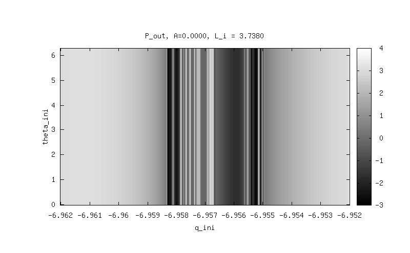
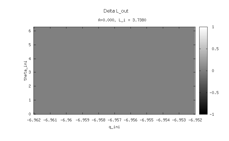
Figure 4: This figure shows the scattering functions $p_{out}(\chi_{in},\psi_{in})$ in the upper part and $\Delta L(\chi_{in},\psi_{in})$ in the lower part for the symmetric case $A=0$. In this symmetric case the angular momentum is a conserved quantity and accordingly $\Delta L\equiv 0$, so the plot appears as homogeneous grey colour. The boundaries of the rectangular domain of these plots should be identified to form a 2 dimensional torus. Note that the fractal structure seen in the upper part of the figure is the Cartesian product of a 1 dimensional fractal in horizontal direction with a circle in vertical direction.

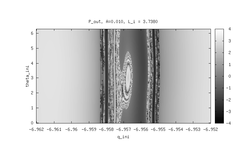
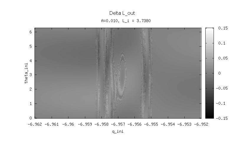
Figure 5: This figure shows the same scattering functions as Fig.4 for the small symmetry breaking $A=0.01$. Because of this symmetry breaking the fractal structure has turned into a truly 2 dimensional fractal. However, a mayor part of the intervals of continuity of the scattering functions still form stripes running in vertical direction. These are qualitative features of the product structure of the symmetric case which have survived the symmetry breaking.

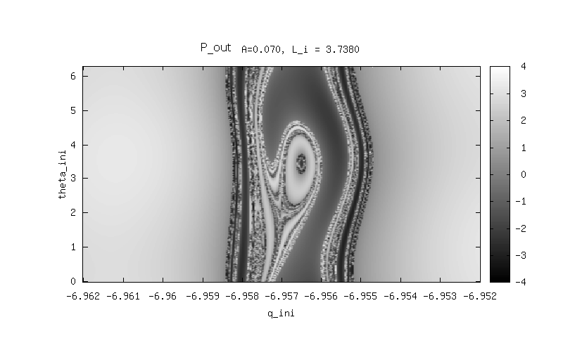
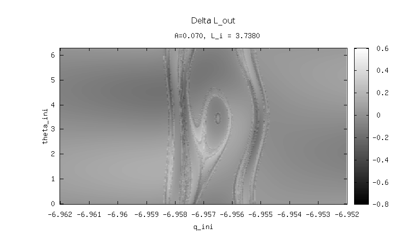
Figure 6: This figure shows the same scattering functions as Figs.4 and 5 for the moderate symmetry breaking $A=0.07$. The intervals of continuity show stronger deformations compared to the symmetric case $A=0$ shown in Fig.4. However, we still see many remnants of the stripes running in vertical direction.

In Figs. 4, 5 and 6 we show an example of this function for three values of A, namely $A=0.0$ in parts a and b, $A=0.1$ in parts c and d and $A=0.3$ in parts e and f. The scattering flow casts a kind of shadow image of the homoclinic tangle into the outgoing asymptotic region and in the scattering functions we see exactly this shadow image. Singularities of the scattering function, i.e. boundaries of intervals of continuity of this function indicate initial conditions on the stable manifold of the NHIM at infinity. Thereby an analysis of the singularities of scattering functions allows the reconstruction of all the important information concerning the chaotic set.

Observe that for $A=0$ the scattering function has a factorization into a fractal structure in $\chi$ direction and constancy in $\psi$ direction. Accordingly the function shows intervals of continuity which are the product of an interval in $\chi$ direction with a circle in $\psi$ direction. For $A$ small only very tiny intervals of continuity of high level of hierarchy change their qualitative structure. The larger intervals keep their basic topology of a strip running around in $\psi$ direction. We have to go to the very strong symmetry breaking of $A\approx 0.5$ to see the largest intervals change their qualitative structure.

4 How the chaotic set appears in the doubly differential cross section

In this section we explain how the fractal chaotic set in phase space or in the Poincaré map causes a fractal pattern of rainbow singularities in the cross section. For the case of three degrees of freedom we generalize the ideas developed in [5] for the case of two degrees of freedom.

Usually in scattering experiments we do not have any control over the relative phase shift variables $\chi$ and $\psi$. We keep $E$, $p_{in}$ and $L_{in}$ fixed and the angles $\chi$ and $\psi$ have a random distribution with constant density on a two dimensional torus. We measure the relative probability to find values $p_{out}$ and $\Delta L$. This quantity properly normalized with respect to the incoming flow is the doubly differential cross section. To calculate this cross section for a particular pair of values of $p_{out}$ and $\Delta L$ we have first to find all the preimages $(\chi_{k},\psi_{k})$ of the scattering function which lead to these particular values of the final variables. Then we have to calculate the determinant

$$d_{k}=det[\partial(p_{out},\Delta L)/\partial(\chi_{in},\psi_{in})]$$ (3)

in the particular initial preimage point k. The cross section is given by

$$\frac{d^{2}\sigma}{dpd\Delta L}(p,\Delta L)=\sum_{preimages}1/|d_{k}|$$ (4)

We see immediately that the cross sections has singularities for such values of $p_{out}$ and $\Delta L$ where the determinant of Eq. 3 is zero. These are values where several preimages collide and disappear, they are projection singularities of the scattering function. These singularities are of one over square root type, therefore the integral over the cross section is finite and there are no problems with flux conservation. As long as the system is close to the symmetric case the scattering function in each interval of continuity is similar to a ring shaped mountain and accordingly the projection singularity of this function looks like the one of half a torus (for details see [8]). Fig. 7 shows the cross section contribution from a single interval of continuity. Fig.8 shows the singularities from the whole toroidal domain of the scattering function. The pattern seen in Fig.8 coincides with what a detector in a real experiment might see. It is a fractal repetition of the basic singularity structure from Fig.7.

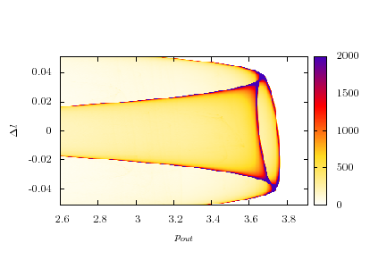
Figure 7: The contribution of a single interval of continuity of the scattering functions ( it is the second largest one seen in Fig.5 ) to the doubly differential cross section defined in Eqs. 3 and 4 for the case $A=0.01$. Note that this figure coincides with the projection of half a torus or of a ring shaped mountain. The caustics of this projection lead to one over square root singularities ( rainbow singularities ) in the cross section.

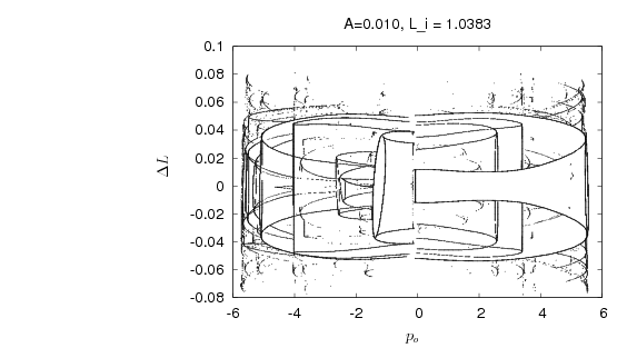
Figure 8: Singularity pattern seen in the doubly differential cross section, again for the case $A=0.01$. In contrast to Fig.7 here the contributions from the complete domain of the scattering functions are included. This pattern of singularity lines is a fractal repetition of the basic pattern created by a single interval of continuity as shown in Fig.7.

We can change a parameter of the system, this might be the symmetry breaking parameter, or a action like initial condition, this might be the incoming angular momentum $L_{ini}$. When we measure the cross section singularities as function of this parameter then we can follow in the cross section the changes of the chaotic set under these changes of the system. This is an interesting contribution to the inverse chaotic scattering problem.

5 Conclusions

The stable manifold of a NHIM at infinity consists of trajectories which go out to infinity while at the same time the longitudinal momentum goes to zero, they are trajectories which arrive at infinity with velocity zero. These manifolds are separatrix surfaces between trajectories going out to infinity and trajectories which return to the interaction region at least once more before eventually also going out to infinity. The trajectories on the unstable manifolds show the same behaviour under time reversal. The homoclinic/heteroclinic tangle between the stable and unstable manifolds of the NHIM at $\pm\infty$ are the higher dimensional generalizations of the horseshoes in two dimensional maps. In our class of systems this chaotic structure exists for all values of the total energy $E$. The reason is that in our class of systems for any value of $E$ there are trajectories going out to infinity with longitudinal velocity zero. This happens thanks to the closed degrees of freedom which can swallow up any amount of energy such that only energy zero is left for the open degree of freedom. In this sense our system is at a channel threshold of the inelastic scattering for any value of $E$.

Because of these considerations it is clear that we do not expect a similar behaviour for scattering systems with open degrees of freedom only. For a discussion of this point for scattering off four hard spheres see [9]. The Poincare map of this system has hyperbolic fixed points but does not have any NHIM.

For systems with more than three degrees of freedom similar considerations hold. For each additional degree of freedom the NHIM and its manifolds acquire two additional neutral directions. The domains of the scattering functions and of the cross section acquire one additional dimension.

References

- [1] S. Smale, Bul. Am. Math. Soc., 73, 747, (1967)
- [2] T. Bütikofer, C. Jung and T. H. Seligman Phys. Lett. A, 76, 265, (2000)
- [3] C. Jung, C. Lipp and T. H. Seligman, Ann. Phys. NY 275, 151 (1999)
- [4] A.B. Schelin, A.P.S de Moura A.P.S and C. Grebogi Phys. Rev. E, 78, 046204, (2008)
- [5] C. Jung, G. Orellana-Rivadeneyra and G. A. Luna, J. Phys. A 38, 567 (2004)
- [6] L. Benet, J. Broch, O. Merlo and T.H. Seligman, Phys. Rev. E 71 (2005), 036225
- [7] S. Wiggins, Normally Hyperbolic Invariant Manifolds in Dynamical Systems, Springer 1994
- [8] C. Jung, O. Merlo, T. H. Seligman and K. Zapfe, N. J. P. In Print.
- [9] Q. Chen, M. Ding and E. Ott, Phys. Lett. A 115, 93 (1990)