Electron spin decoherence in diluted magnetic quantum wells

Abstract

We study electron spin dynamics in diluted magnetic quantum wells. The electrons are coupled by exchange interaction with randomly distributed magnetic ions polarized by magnetic field $\mathbf{B}.$ This coupling leads to both spin relaxation and spin decoherence. We demonstrate that even very small spatial fluctuations of quantum well width dramatically increase rate of decoherence. Depending on the strength of exchange interaction and the amplitude of the fluctuations the decoherence can be homogeneous or inhomogeneous. In the homogeneous regime, the transverse (with respect to $\mathbf{B}$) component of electron spin decays on the short time scale exponentialy while the long-time spin dynamics is non-exponential demonstrating long-lived power law tail. In the inhomogeneous case, the transverse spin component decays exponentially with the exponent quadratic in time.

Effective manipulation of spin degree of freedom in a semiconductor device by external electric and magnetic fields is one of the primary goals of spintronics. avsh A possible way to increase coupling of electron spin to external magnetic field is to use semiconductor-based materials, which incorporate magnetic elements. Such materials are called diluted magnetic semiconductors (DMS). The most common DMS are II-VI and IV-VI compounds with magnetic impurities (usually, Mn), and also III-V crystals, 4 ; 5 like Ga_1-xMn_xAs (typically, $x<10\%$). The DMS combine magnetic and semiconductor properties in a single material. This offers a large prospect for applications. In particular, DMS are considered to be the most promising candidates in creating room-temperature ferromagnetic systems, which can be easily manipulated as semiconductors. Semiconductor heterostructures doped by magnetic impurities have already demonstrated exciting physical phenomena specific for magnetic systems: coherent spin excitations, a3 ; a4 magnetic polaron formation, a5 ferromagnetic hole alignment, a6 etc.

Many remarkable features of DMS, such as the large Zeeman splitting of the electronic bands and the giant Faraday rotation, are induced by the exchange interaction between the localized electrons on d-shells of Mn ions and delocalized band carriers (see Ref. dyak, for review). This interaction is also responsible for the collective nature of spin excitations in DMS, arising of novel collective modes, 6 ; 8 , anticrossing of the electron and ion spin precession frequencies, 6 ; 1 spin susceptibility enhancement, 7 etc.

The fluctuations of exchange field around the average value lead to electron spin relaxation and spin decoherence with characteristic times $T_{1}$ and $T_{2},$ respectively. Recently, the decoherence rate was measured in Cd_1-xMn_xTe two-dimensional (2D) structure. 2 The observed $T_{2}$ was found to be at least one order magnitude shorter than the decoherence time predicted theoretically in Ref. 3, , where fluctuations of exchange field were linked to delta-correlated fluctuations of magnetic ion concentration. In this paper, we demonstrate that even very small fluctuations of quantum well width dramatically increase rate of decoherence. Our estimates show that this mechanism can explain short decoherence time observed in Ref. 2, .

We consider the 2D degenerate electron gas located in the $(x,y)$ plane interacting with the magnetic ions randomly distributed with average 2D concentration $n_{J}$, and doping profile $f(z)$ in the growth direction $(\int f(z)dz=1)$. The system is placed into the magnetic field which we assume to be parallel to the well plane ($\mathbf{B}\parallel\mathbf{e}_{x}$) as it was the case in Ref. 2, . The field leads to Zeeman splitting of both electron and ion spin levels with energies $\hbar\omega_{e}$ and $\hbar\omega_{J},$ respectively. The Hamiltonian of the system is given by

$$\hat{H}=\hat{H}_{e}+\hat{H}_{J}+\hat{H}_{Je},$$ (1)

$$\hat{H}_{e}=\frac{\mathbf{p}^{2}}{2m}+U(\mathbf{r})+\hbar\omega_{e}\hat{s}_{x},$$ (2)

$$\hat{H}_{J}=\hbar\omega_{J}\sum_{k}{\hat{J}_{kx}},$$ (3)

$$\hat{H}_{Je}=\alpha\mathbf{\hat{s}}\sum_{k}{\mathbf{\hat{J}}_{k}\delta(\mathbf{r}-\mathbf{R}_{k})}|\Psi(z_{k})|^{2}.$$ (4)

Here $\hat{H}_{e}$ is the Hamiltonian of an electron in the external magnetic field, $\mathbf{r}=(x,y)$ and $\mathbf{p}=(p_{x},p_{y})$ are respectively electron in-plane position vector and momentum, $U(\mathbf{r})$ is the random impurity potential, which we assume to be short-range, $\hat{H}_{J}$ is the Hamiltonian of the ions and $\hat{H}_{Je}$ represents the exchange interaction between spin $\mathbf{s}$ of an electron placed at the lowest level in the well (with the wave function $\Psi(z)$) and the spins $\mathbf{J}_{k}$ of the ions located at points $(\mathbf{R}_{k},z_{k})$. The strength of the interaction is characterized by constant $\alpha.$

It is convinient to rewrite $\hat{H}_{Je}$ as

$$\hat{H}_{Je}=\langle\hat{H}_{Je}\rangle+\delta\hat{H}_{Je},$$ (5)

where the angular brackets mean averaging over ion positions and thermal averaging and $\delta\hat{H}_{Je}$ describes fluctuations of exchange field. The term $\langle\hat{H}_{Je}\rangle$ leads to significant renormalization of the electron spin precession frequency

$$\omega=\omega_{e}+\frac{\alpha\langle J_{x}\rangle n_{J}}{\hbar}\int f(z)|\Psi(z)|^{2}dz,$$ (6)

Typically, $\omega\gg\omega_{e}$,1 ; 2 which means that the electron spin precession frequency is mostly determined by the effective magnetic field, created by polarized ions.

The fluctuations of the exchage field arising due to random distribution of $(R_{k},z_{k})$ lead both to electron spin relaxation and to decoherence. The analysis of these processes shows 3 that in 2D case the longitudinal and transverse (with respect to $\mathbf{B}$) components of the electron spin decay exponentially with the characteristic times $T_{1}^{\prime}\sim T_{2}^{\prime}\sim{2a^{2}\hbar^{3}}/{3\alpha^{2}mn_{J}}.$ Comparing the results of Ref. 3, with the recent experimental data, 2 one can see that experimentally observed decoherence time $T_{2}$ is much shorter (by about an order of magnitude) than $T_{2}^{\prime}$, which implies that delta-correlated density fluctuations can not provide sufficient fluctuations of the exchange field.

Below we demonstrate that spatial fluctuations of quantum well width can (at certain conditions) lead to significantly shorter $T_{2}$. Physically, this happens because such fluctuations induce the long-range fluctuations of the effective magnetic field acting on the electron spin.

First, we notice that the effective magnetic field induced by exchange interaction depends on the doping profile $f(z)$ and quantum well geometry (see Eq. (6)). Expressions for $T_{1}^{\prime}$ and $T_{2}^{\prime}$ were derived 3 for the case of homogeneous distribution of magnetic ion and infinitely deep quantum well, having constant width $a_{0}.$ Let us now assume, for example, that the quantum well is infinitely deep and magnetic ions concentrate close to the center of the well (these assumptions more or less correspond to the experimental situation 2 ). Assuming also that well width slightly fluctuates, $a(\mathbf{r})=a_{0}+\delta a(\mathbf{r})$ we find that spin precession frequency becomes $\mathbf{r}-$dependent:

$$\omega\rightarrow\omega(\mathbf{r})=\omega_{e}+\frac{2\alpha\langle J_{x}\rangle n_{J}}{\hbar a(\mathbf{r})}=\omega_{0}+\delta\omega(\mathbf{r}),$$ (7)

where $\omega_{0}=\omega_{e}+{2\alpha\langle J_{x}\rangle n_{J}}/{\hbar a_{0}},$ $\delta\omega(\mathbf{r})\approx-{2\alpha\langle J_{x}\rangle n_{J}\delta a(\mathbf{r})}/{\hbar a_{0}^{2}}.$ We assume the fluctuations to be Gaussian with a spatial scale $d$:

$$\langle\delta\omega(\mathbf{r})\delta\omega(\mathbf{r^{\prime}})\rangle=2\omega^{2}_{*}\,\chi\left(\frac{|\mathbf{r}-\mathbf{r}^{\prime}|}{d}\right).$$ (8)

Here $\omega_{*}^{2}={2\alpha^{2}\langle J_{x}\rangle^{2}n_{J}^{2}}{\langle\delta a^{2}(\mathbf{r})\rangle}/\hbar^{2}{a_{0}^{4}}$ is the amplitude of the flucuations and $\chi(\xi)$ is a dimensionless function ($\chi(0)=1,~{}\chi(\xi)\to 0,~{}{\rm for}~{}\xi\gg 1$). As seen from Eq. (8), $\langle\delta\omega(\mathbf{r})\delta\omega(\mathbf{r^{\prime}})\rangle\sim\langle J_{x}\rangle^{2},$ so that at low magnetic fields the fluctuations vanish and decoherence is due to the mechanism proposed in Ref. 3, . However, at relatively strong fields corresponding to almost full polarization of ions (this was the case in the experiment 2 ) the fluctuations are sufficiently large and dominate the decoherence.

We will consider time evolution of the spin excitations concentrated near Fermi surface. The total transverse spin (per unit area) can be written as $S_{+}(t)=S_{y}+iS_{z}=e^{i\omega_{0}t}S(t),$ where $S(t)=\int s_{+}(\mathbf{r},\varphi,t)d\varphi d^{2}\mathbf{r}/\Omega$ is slowly decaying amplitude, $\Omega$ is the sample area and $s_{+}=s_{y}+is_{z}$ is the spin density that obeys the following quasiclassical kinetic equation dyakonov_old ; dyakonov_new

$$\frac{\partial s_{+}}{\partial t}+v_{F}\mathbf{n}\frac{\partial s_{+}}{\partial\mathbf{r}}-i\delta\omega(\mathbf{r})s_{+}=\mathrm{{St}}\{s_{+}\},$$ (9)

where $\varphi$ is the velocity angle, $v_{F}$ is the Fermi velocity $\mathbf{n}=\mathbf{e}_{x}\cos\varphi+\mathbf{e}_{y}\sin\varphi,$ and $\mathrm{St}\{s_{+}\}$ is the collision integral describing the elastic scattering on the impurity potential $U(\mathbf{r})$ with the mean free path $l$. The quasiclassical approach based on Eq. (9) is valid provided that $d\gg\hbar/mv_{F}$ and $\hbar\omega(\mathbf{r})\ll mv_{F}^{2}.$ Below we will solve this equation with the initial condition $s_{+}(\mathbf{r},\varphi,0)=1.$

The spin decoherence can be homogeneous or inhomogeneous depending on the parameter $\omega_{*}\tau,$ where $\tau$ is a characteristic time required for electron to travel the distance of the order of $d.$ For $d\ll l$, this time is given by $\tau=d/v_{F},$ while for $d\gg l$, $\tau=d^{2}/4D\sim d^{2}/lv_{F},$ where $D=v_{F}l/2$ is the diffusion coefficient.

For $\omega_{*}\tau\gg 1,$ electron spins in different correlation regions rotate independently with local frequencies. Hence, the decoherence is inhomogeneous and the transverse spin decays as

$$S(t)\approx\langle e^{i\delta\omega(\mathbf{r})t}\rangle=e^{-{\omega_{*}^{2}t^{2}}}.$$ (10)

In the opposite case, $\omega_{*}\tau\ll 1,$ electron is visiting many correlated regions during decoherence time and the decoherence is homogeneous. First, we assume $d\ll l.$ If the inequality $T_{2}v_{F}\ll l$ is also satisfied, the electron motion on the time scale on the order of $T_{2}$ is ballistic. Neglecting the collision integral in Eq. (9), we obtain

$$S(t)=\left\langle e^{i\int_{0}^{t}\delta\omega(v_{F}\mathbf{n}\tau)\mathrm{d}\tau}\right\rangle$$ (11)

$$=e^{-\omega_{*}^{2}\int_{0}^{t}\int_{0}^{t}\chi(v_{F}|\tau_{1}-\tau_{2}|/d)\mathrm{d}\tau_{1}\mathrm{d}\tau_{2}}.$$

For $t\gg d/v_{F}$, Eq. (11) becomes

$$S(t)=e^{-t/T_{2}},~{}\frac{1}{T_{2}}=\frac{2\omega_{*}^{2}d}{v_{F}}\int\limits_{0}^{\infty}{\chi(\xi)\mathrm{d}\xi}.$$ (12)

It turns out that Eq. (12) is also valid for $T_{2}v_{F}\gg l.$ To see this, one can iterate Eq. (9) with respect to small $\delta\omega$ and decouple correlations, which yields $1/T_{2}=\int d\mathbf{r}^{\prime}\int dt^{\prime}\langle\delta\omega(\mathbf{r})G(\mathbf{r}-\mathbf{r}^{\prime},t-t^{\prime})\delta\omega(\mathbf{r}^{\prime})\rangle.$ Here $G(\mathbf{r},t)$ is the Green function of Eq. (9) with $\delta\omega(\mathbf{r})=0$ (Green function of the Boltzmann equation) integrated over initial velocity directions and averaged over final velocity directions. This function can be presented as a sum over processes with different number of collisions: $G(\mathbf{r},t)=\langle\delta(\mathbf{r}-v_{F}\mathbf{n}t)\rangle_{\varphi}\exp(-tv_{F}/l)+\sum_{N=1}^{\infty}G_{N}(\mathbf{r},t),$ where the first term is the ballistic contribution, which gives Eq. (12). Relative contribution of other terms to $1/T_{2}$ (compared to Eq. (12)) may be shown to be on the order of parameter $(d/l)\ln(1/\omega_{*}\tau)\ll 1$.com

For $d\gg l$ and $\omega_{*}\tau=\omega_{*}d^{2}/4D\ll 1,$ the decoherence is also homogeneous. In this case the electron motion is diffusive and one can by standard means reduce Eq. (9) to diffusion equation:

$$\frac{\partial s_{+}}{\partial t}-D\Delta s_{+}-i\delta\omega(\mathbf{r})s_{+}=0.$$ (13)

Iterating Eq. (13) with respect to $\delta\omega$ and decoupling correlations, we obtain

$$\frac{\partial s_{+}}{\partial t}-D\Delta s_{+}+\int d\mathbf{r}^{\prime}dt^{\prime}\Lambda_{\mathbf{r}-\mathbf{r}^{\prime},t-t^{\prime}}s_{+}(\mathbf{r}^{\prime},t^{\prime})=0,$$ (14)

where

$$\Lambda_{\mathbf{r}-\mathbf{r}^{\prime},t-t^{\prime}}=2\omega^{2}_{*}\chi\left(\frac{|\mathbf{r}-\mathbf{r}^{\prime}|}{d}\right)G_{D}(\mathbf{r}-\mathbf{r}^{\prime},t-t^{\prime}),$$

and $\hat{G}_{D}=(\partial/\partial t-D\Delta)^{-1}$ is the Green function of the diffusion equation. Solving Eq. (14) with the initial condition $s_{+}(\mathbf{r},\varphi,0)=1$, we find

$$S(t)=\int_{-\infty}^{\infty}{\frac{d\omega}{2\pi}\frac{e^{-i\omega t}}{-i\omega+2\omega_{*}^{2}d^{2}\int_{0}^{\infty}\frac{\tilde{\chi}(qd)}{Dq^{2}-i\omega}{\frac{qdq}{2\pi}}}},$$ (15)

where $\tilde{\chi}$ is the Fourier transform of $\chi$.

Figure 1: Decay of the transverse spin amplitude in the diffusive case

The integrand in Eq. (15) has two poles and a branch cut along the negative imaginary axis. The poles are at the points $\omega_{1,2}\approx({2\tilde{\chi}(0)\omega_{*}^{2}\tau}/{\pi})\left[\pm\pi-2i\ln\left({1}/{\omega_{*}\tau}\right)\right],$ where $\tau=d^{2}/4D,\tilde{\chi}(0)=2\pi\int_{0}^{\infty}\xi\chi(\xi)d\xi$.

Figure 2: Decoherence rate as a function of the correlation radius of the fluctuations. For $d>d_{0}$ mechanism related to fluctuations of the well width dominates

The imaginary parts of the poles are large compared to the real ones, so that the poles contribution is approximately given by

$$S(t)\approx\exp\left[-\frac{4\tilde{\chi}(0)\omega_{*}^{2}\tau t}{\pi}\ln\left(\frac{1}{\omega_{*}\tau}\right)\right].$$ (16)

This contribution dominates at short times, $\omega_{*}^{2}\tau t\ll 1.$ For $\omega_{*}^{2}\tau t\gg 1,$ the main contribution is due to branch cut, yielding

$$S(t)\approx-\frac{\pi}{2\tilde{\chi}(0)}\frac{1}{\omega_{*}^{2}\tau t\,\ln^{2}\left(t/\tau\right)}.$$ (17)

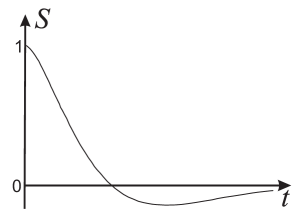
The contribution of the branch cut is negative. From Eqs. (16) and (17) we see that the amplitude $S(t)$ changes sign as shown in Fig. 1. We also see that a long-lived power-law tail appears in the transverse spin polarization.

Above we assumed that $\mathbf{B}$ is parallel to the well plane and neglected the effect of the field on the orbital motion. The results are also valid for $\mathbf{B}\parallel\mathbf{e}_{z}$ provided that $R_{c}\gg l$ ($R_{c}$ is the cyclotron radius). Our calculations can be easily generalized for the opposite case, $R_{c}\ll l$. In particular, in the homogeneous ballistic regime, under the assumptions $\omega_{*}\tau\ll 1,d\ll R_{c}\ll l,R_{c}\ll T_{2}v_{F}\ll l$, the transverse spin can be calculated in analogy with Eq. (11) by averaging of decoherence action calculated along ballistic trajectory. The result looks com1

$$S(t)=e^{-t^{2}/T_{2}^{2}},~{}\frac{1}{T_{2}^{2}}=\frac{\omega_{*}^{2}d}{\pi R_{c}}\int\limits_{0}^{\infty}{\chi(\xi)\mathrm{d}\xi}.$$ (18)

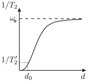
From equations derived above one can see that increasing correlation radius $d$ decreases $T_{2}$ both for $d\ll l$ and for $d\gg l$. The maximal value of $1/T_{2}$ is on the order of $\omega_{*}.$ One can show that $\omega_{*}T_{2}^{\prime}\gg 1$ for typical values of parameters,2 which implies that suggested mechanism dominates already at small $d$ ($d>d_{0}$, see Fig. 2) and might be responsible for short values of decoherence time observed in the experiment.2 The parameter $d_{0}$ is estimated as follows: $d_{0}\sim{k_{F}a^{2}}/{n_{J}\delta a_{0}^{2}},$ for $l\gg d$ and $d_{0}\sim\sqrt{{k_{F}a^{2}l}/{n_{J}\delta a_{0}^{2}},}$ for $l\ll d$ regime. Taking $\delta a_{0}=\sqrt{\langle\delta a^{2}(\mathbf{r})\rangle}$ on the order of the lattice constant, for typical values of experimental parameters 2 we find that $d_{0}\approx 10nm$.
We thank M. Glazov for useful discussion. The work was supported by RFBR, by grant of Russian Scientific School, by the Grant of Rosnauka (project number 02.740.11.5072) and by programmes of the RAS. V.Yu.K. was supported by Dynasty foundation.

References

- (1) 467 Semiconductor Spintronics and Quantum Computation, eds. D.D. Awschalom, D. Loss, and N. Samarth, in the series ”Nanoscience and technology”, eds. K. von Klitzing, H. Sakaki, and R. Wiesendanger (Springer, Berlin, 2002).
- (2) Y. Ohno, D.K. Young, B. Beschoten, F. Matsukura, H. Ohno, and D.D. Awschalom, Nature (London) 402, 790 (1999).
- (3) M. Tanaka and Y. Higo, Phys.Rev. Lett. 87, 026602 (2001).
- (4) S.A. Crooker, J.J. Baumberg, F. Flack, N. Samarth, and D.D. Awschalom, Phys. Rev. Lett. 77, 2814 (1996).
- (5) J. Sthler, G. Schaack, M. Dahl, A. Waag, and G. Landwehr, K.V. Kavokin, I.A. Merkulov, Phys. Rev. Lett. 74, 2567 (1995).
- (6) D.R. Yakovlev and K.V. Kavokin, Comments Condens. Matter Phys. 18, 51 (1996).
- (7) A. Haury, A. Wasiela, A. Arnoult, J. Cibert, S. Tatarenko, T. Dietl, and Y. M. d’Aubigne, Phys. Rev. Lett. 79, 511 (1997).
- (8) J. Cibert and D. Scalbert ”Diluted Magnetic Semiconductors: Basic Physics and Optical Properties”, in ”Spin Physics in Semiconductors”, ed. by M.I. Dyakonov (Berlin, Springer, 2008) chap. 13.
- (9) J. Konig and A.H. MacDonald, Phys. Rev. Lett. 91, 077202 (2003).
- (10) D. Frustaglia, J. Konig, and A.H. MacDonald, Phys. Rev. B 70, 045205 (2004).
- (11) F.J. Teran, M. Potemski, D.K. Maude, D. Plantier, A.K. Hassan, A. Sachrajda, Z. Wilamowski, J. Jaroszynski, T. Wojtowicz, and G. Karczewski, Phys. Rev. Lett. 91, 077201 (2003).
- (12) F. Perez, C. Aku-leh, D. Richards, B. Jusserand, L.C. Smith, D. Wolverson, and G. Karczewski, Phys. Rev. Lett. 99, 026403 (2007).
- (13) M. Vladimirova, S. Cronenberger, P. Barate, D. Scalbert, F.J. Teran, A.P. Dmitriev, Phys. Rev. B 78, 081305(R) (2008).
- (14) Y.G. Semenov, Phys. Rev. B 67, 115319 (2003).
- (15) M.I. Dyakonov, V.I. Perel, Sov. Phys. JETP Lett. 13, 467 (1971)
- (16) M.I. Dyakonov, Physica E 35, 246 (2006).
- (17) We do not consider here intermediate case
- (18) The quadratic dependence of decoherence exponent on time (decoherence acceleration) is analogous to the acceleration of the spin relaxation in a system with random spin-orbit coupling. glazov
- (19) M.M. Glazov and E. Ya. Sherman, Phys. Rev. B 71, 241312(R) (2005)