Embedding punctured $n$-manifolds in Euclidean $(2n-1)$-space

Abstract.

Let $N$ be a closed orientable connected $n$-manifold, $n\geq 4$. We classify embeddings of the punctured manifold $N_{0}$ into $\mathbb{R}^{2n-1}$ up to isotopy. Our result in some sense extends results of J.C. Becker – H.H. Glover (1971) and O. Saeki (1999).

1. Introduction and main results

This paper is on the classical Knotting Problem: for a manifold $N$ and a number $m$ describe the set $\mathrm{Emb}^{m}(N)$ of isotopy classes of embeddings $N\to\mathbb{R}^{m}$. For recent surveys, see [Sk06, HCEC].

We classify embeddings of the punctured $n$-manifold $N_{0}$ into $\mathbb{R}^{2n-1}$ up to isotopy.

Unless otherwise stated, we work in the PL (piecewise linear) or DIFF (smooth) category and the results are valid in both categories. For a manifold $X$ we denote by $\mathrm{Emb}^{s}X$ the set of isotopy classes of embeddings $X\to\mathbb{R}^{s}$, and by $X_{0}$ we denote $X$ minus the interior of a codimension 0 open ball.

Let $N$ be a closed orientable connected $n$-manifold. For $n\geq 6$ the set $\mathrm{Emb}^{2n-1}N$ was described in [Ya84], see also [Sk10]. For $n=3$ and $H_{1}(N)$ torsion-free, $\mathrm{Emb}^{2n-1}N_{0}=\mathrm{Emb}^{5}N_{0}$ was described by Saeki [Sa99], see below. The method of [Sa99] used classification of normal bundles of embeddings $N_{0}\to\mathbb{R}^{5}$ and could not be directly generalized on higher dimensions. Our main result is Theorem 1 below which implies a description of $\mathrm{Emb}^{2n-1}N_{0}$ for $n\geq 4$, see Corollary 1.

If (co)homology coefficients are omitted, they are assumed to be $\mathbb{Z}$. We denote $\mathbb{Z}_{(n)}:=\mathbb{Z}$ when $n$ is even and $\mathbb{Z}_{(n)}:=\mathbb{Z}_{2}$ when $n$ is odd. For an abelian group $G$ denote by $B_{s}(G)$ the group of symmetric (for $s$ even) or antisymmetric (for $s$ odd) elements of $G^{\otimes 2}:=G\otimes_{\mathbb{Z}}G$.

Corollary 1. Let $N$ be a closed connected orientable $n$-manifold, $n\geq 4$. Then, as sets,

$$\mathrm{Emb}^{2n-1}N_{0}=A\times H_{1}(N;\mathbb{Z}_{(n-1)})$$

where $A$ is a quotient set of $H_{1}(N)^{\otimes 2}$.

We also present a sketch of proof of the following conjecture, a detailed proof of which will appear in a subsequent version of the paper.

Conjecture 1. Let $N$ be a closed connected orientable $n$-manifold, $n\geq 4$. Then, as sets,

$$\mathrm{Emb}^{2n-1}N_{0}=B_{n}(H_{1}(N))\times H_{1}(N;\mathbb{Z}_{(n-1)}).$$

Define the cone map

$$\Lambda:\mathrm{Emb}^{m}(N_{0})\to\mathrm{Emb}^{m+1}(N)$$

which adds a cone over $\partial N_{0}$, see figure 1. This map is well-defined in the PL category and for $m\geq 3n/2+1$ in the smooth category.

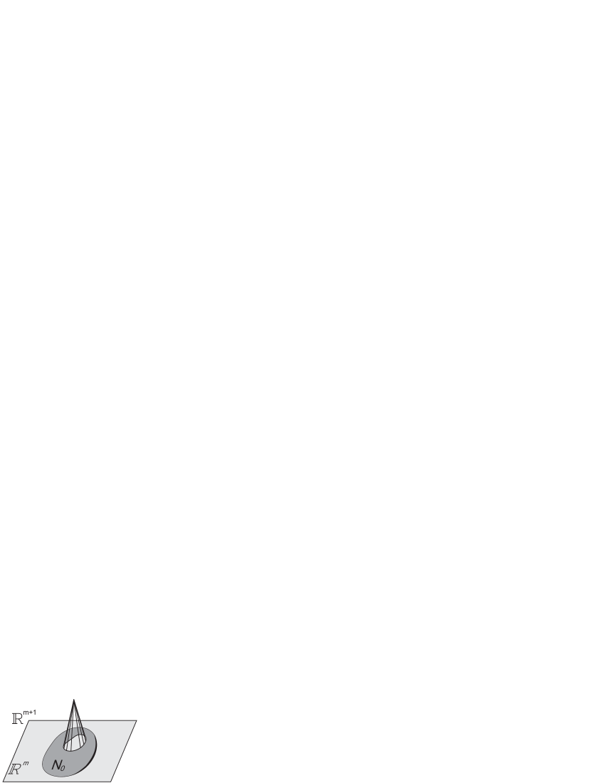
Figure 1. The cone map $\Lambda$ which adds a cone to an embedding of $N_{0}$.

Theorem 1. Let $N$ be a closed homologically $k$-connected orientable $n$-manifold, $n\geq 4k+4$, $k\geq 0$. Then the cone map $\Lambda:\mathrm{Emb}^{2n-2k-1}N_{0}\to\mathrm{Emb}^{2n-2k}N$ is surjective and the preimage $\lambda^{-1}x$ of each element is in 1-1 correspondence with a quotient set of $H_{k+1}(N)^{\otimes 2}$.

In other words, there is the following exact sequence of sets with an action $a$.

$$\begin{CD}H_{k+1}(N)^{\otimes 2}@>{a}>{}>\mathrm{Emb}^{2n-2k-1}N_{0}@>{\Lambda}>{}>\mathrm{Emb}^{2n-2k}N@>{}>{}>0.\end{CD}$$

The surjectivity of $\Lambda$ in Main Theorem 1 was known, see Theorem 2 below (compare [Vr89, Corollary 3.3]). Our main result in Theorem 1 is the estimation of the ‘kernel’ of the cone map $\Lambda$.

The Becker–Glover Theorem 2. [BG71] Let $N$ be a closed homologically $k$-connected $n$-manifold and $m\geq 3n/2+2$. The cone map $\Lambda:\mathrm{Emb}^{m}(N_{0})\to\mathrm{Emb}^{m+1}(N)$ is one-to-one for $m\geq 2n-2k$ and is surjective for $m=2n-2k-1$.

Analogously to Theorem 1 we could prove that there is an exact sequence with an action $a$

$$\begin{CD}B_{3}(H_{1}(N))@>{a}>{}>\mathrm{Emb}^{5}N_{0}@>{}>{}>H_{1}(N,\mathbb{Z})@>{}>{}>0.\end{CD}$$

in the DIFF category. This result for $H_{1}(N)$ torsion free is known [Sa99]. Moreover, in this case each stabilizer of the action $a$ is in 1-1 correspondence with $I_{N}:=\{\iota_{a}(\mu):=\cdot\cap\cdot\cap a\ |\ a\in H_{1}(M)\}\subset B_{3}(H_{1}(N))$ where $\mu:H_{1}(N)\times H_{1}(N)\times H_{1}(N)\to\mathbb{Z}$ is the intersection form. In other words, the preimage of $\Lambda$ is in 1-1 correspondence with $H_{1}(N)\times B_{3}(H_{1}(N))/I_{N}$.

We conjecture there is a geometric construction of the invariant $\mathrm{Emb}^{2n-1}N_{0}\to H_{1}(N)^{\otimes 2}$ implicitly obtained in Corollary 1. If $N$ is a connected sum of several $(S_{1}\times S^{n-1})$’s then the pairwise linking coefficients $\mathrm{lk}(*\times S^{n-1}_{i},*\times S^{n-1}_{j})$ provide such an invariant if we take into account that $H_{1}(N)\cong H_{n-1}(N)$ in this case (the invariant will actually be in $B_{n}(H_{1}(N))$). In the general case, even if $H_{1}(N)$ is free, the linking coefficient is harder to define since $(n-1)$- cycles of $N_{0}$ may intersect each other.

Proof of Corollary 1. Corollary 1 follows from Theorem 1(a) and the fact there is a bijection $\mathrm{Emb}^{2n}N\to H_{1}(N,\mathbb{Z}_{(n-1)})$, the Whitney invariant [EBSR]. $\blacksquare$

2. Proof of Theorem 1

Proof of Theorem 1 for $k=0$. Denote $m=2n-2k$. Consider the following commutative diagram of sets, in which the horizontal maps are bijections.

$$\begin{CD}\mathrm{Emb}^{m}(N)\begin{picture}(1.0,10.0)\put(-65.0,3.0){\vector(1,0){130.0}} \end{picture}^{\alpha}\pi_{\mathrm{eq}}^{m-1}(\widetilde{N})\\ @A{\Lambda}A{}A@A{\lambda^{\star}}A{}A\\ \mathrm{Emb}^{m-1}(N_{0})@>{\alpha_{0}}>{}>\pi_{\mathrm{eq}}^{m-2}(\widetilde{N_{0}})@>{\Sigma}>{}>\pi_{\mathrm{eq}}^{m-1}(\Sigma\widetilde{N_{0}})\end{CD}$$

Here

$\bullet$ $\widetilde{N}$ is the deleted product of $N$, i.e. $N^{2}$ minus an open tubular neighborhood of the diagonal, with standard involution;

$\bullet$ $\pi^{i}_{\mathrm{eq}}X$ is the set of equivariant maps $X\to S^{i}$ up to equivariant homotopy.

$\bullet$ maps $\alpha$ and $\alpha_{0}$ are the Haefliger-Wu invariants [Sk06, 5.2].

$\bullet$ $\Sigma$ is the suspension;

$\bullet$ $\lambda^{*}$ is induced by an equivariant map $\lambda:\widetilde{N}\to\Sigma\widetilde{N_{0}}$ defined below.

Construction of $\lambda$.

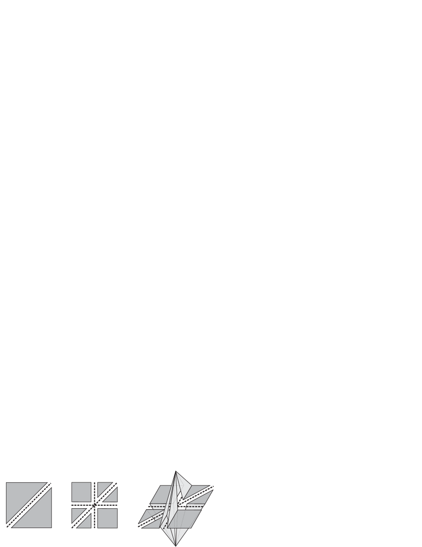
Figure 2. From left to right: $\widetilde{N}$, $\widetilde{N_{0}}$ and the image $\lambda\widetilde{N}\subset\Sigma\widetilde{N_{0}}$.

We repeat the construction of [BG71]. Represent

(1) $$\Sigma\widetilde{N_{0}}=\frac{\widetilde{N_{0}}\times[-1;1]}{\widetilde{N_{0}}\times\{-1\},\ \widetilde{N_{0}}\times\{1\}}.$$

For $x\in\widetilde{N_{0}}$ set $\lambda(x):=(x,0)$. We identify $U_{\varepsilon}(P)$ with the unit ball in $\mathbb{R}^{n}$, with $P$ corresponding to $0\in\mathbb{R}^{n}$. Now set (see figure 2)

$$\lambda(x):=((x_{1},v),t-1)\quad\mathrm{for}\quad x=(x_{1},tv)\in N_{0}\times U_{\varepsilon}(P)\quad\mbox{where}\quad x_{1}\in N_{0};\quad v\in\partial U_{\varepsilon}(P);\quad t\in[0;1].$$

Analogously, for $x=(tv,x_{1})\in B^{n}\times N_{0}$ set $\lambda(x):=((x_{1},v),1-t)$.

Proof of commutativity of the diagram above. Consider an embedding $f:N_{0}\subset\mathbb{R}^{m-1}$. It induces an equivariant map $f_{*}:\widetilde{N_{0}}\to S^{m-2}$. By definition of the Haefliger-Wu invariant, $[f_{*}]=\alpha_{0}[f]$. Next, $\Lambda f$ induces an equivariant map $(\Lambda f)_{*}:\widetilde{N}\to S^{m-1}$, $[(\Lambda f)_{*}]=\alpha\Lambda[f]$. The commutativity of the diagram above is equivalent to the following fact: the map $(\Lambda f)_{*}$ is equivariantly homotopic to the composition

$$\widetilde{N}\stackrel{{\scriptstyle\lambda}}{{\to}}\Sigma\widetilde{N_{0}}\stackrel{{\scriptstyle\Sigma f_{*}}}{{\to}}S^{m-1}.$$

The maps $(\Lambda f)_{*}$ and $(\Sigma f_{*})\lambda$ coincide on $\widetilde{N_{0}}$, both send the ‘vertical’ component $B^{n}\times N_{0}$ of $\widetilde{N}\setminus\widetilde{N_{0}}$ to the upper hemisphere of $S^{m-1}$ and the ‘horizontal’ component $N_{0}\times B^{n}$ to the lower hemisphere. Thus $((\Sigma f_{*})\lambda)(x)\in S^{m-1}$ and $(\Lambda f)_{*}(x)\in S^{m-1}$ are not antipodal for each $x\in\widetilde{N}$, meaning that $(\Sigma f_{*})\lambda$ and $(\Lambda f)_{*}$ are equivariantly homotopic. $\blacksquare$

The map $\alpha$ is one-to-one by the Haefliger-Weber theorem [Ha63, We67], [Sk06, 5.2 and 5.4]. The map $\alpha_{0}$ is one-to-one by the the Haefliger theorem for manifolds with boundary (see [Ha63, 6.4], [Sk02, Theorem 1.1$\alpha\partial$] for the DIFF case and [Sk02, Theorem 1.3$\alpha\partial$] for the PL case). Next, $\Sigma$ is one-to-one by the equivariant version of Freudenthal suspension theorem [CF60, Theorem 2.5].

It remains to prove that $\lambda^{*}$ is surjective and each preimage ${\lambda^{*}}^{-1}f_{0}$ is in 1-1 correspondence with a quotient set of $H_{k+1}(N)^{\otimes 2}$ for each $f_{0}\in\pi_{\mathrm{eq}}^{m-1}(\widetilde{N})$. We will need the following assertion which is proved below.

Assertion 1. For a $k$-connected $n$-manifold and the constructed $\lambda$ consider the equivariant cohomology groups $H^{*}_{\mathrm{eq}}(\Sigma\widetilde{N_{0}},\lambda\widetilde{N})$, with respect to the trivial action of $\mathbb{Z}_{2}$ on $\mathbb{Z}$-coefficients. Then

(a) for $i\leq 2k$ we get $H^{2n-i}_{\mathrm{eq}}(\Sigma\widetilde{N_{0}},\lambda\widetilde{N})=0$;

(b) $H^{2n-2k-1}_{\mathrm{eq}}(\Sigma\widetilde{N_{0}},\lambda\widetilde{N})\cong H_{k+1}(N)^{\otimes 2}$.

There is a 1-1 correspondence between $\pi^{m-1}_{\mathrm{eq}}\widetilde{N}$ and $\pi^{m-1}_{\mathrm{eq}}\lambda\widetilde{N}$ since $\lambda$ is not injective only on some cells of dimension $n<m-2$. We will thus work with $\pi^{m-1}_{\mathrm{eq}}\lambda\widetilde{N}$ and $\pi^{m-1}_{\mathrm{eq}}\widetilde{N}$ interchangeably. Take an equivariant map $f_{0}:\lambda\widetilde{N}\to S^{m-1}$. It can be extended to an equivariant map $f_{1}:\Sigma\widetilde{N_{0}}\to S^{m-1}$ since by Assertion 1(a),

$$H^{i}_{\mathrm{eq}}(\Sigma\widetilde{N_{0}},\lambda\widetilde{N};\pi_{i-1}S^{m-1})=0\quad\mbox{for each }i.$$

This proves that $\lambda^{*}$ is surjective.

Fix an extension $f_{1}:\Sigma\widetilde{N_{0}}\to S^{m-1}$ of $f_{0}$. Denote by $\pi_{\mathrm{eq}}^{m-1}(\Sigma\widetilde{N_{0}},\lambda\widetilde{N})$ the set of equivariant extensions of $f_{0}$ on $\Sigma\widetilde{N_{0}}$ up to equivariant homotopy fixed on $\lambda\widetilde{N}$. Consider the following diagram.

$$\begin{CD}0\\ @A{}A{}A\\ \pi_{\mathrm{eq}}^{m-1}(\widetilde{N})\\ @A{\lambda^{*}}A{}A\\ \pi_{\mathrm{eq}}^{m-1}(\Sigma\widetilde{N_{0}})\\ @A{j}A{}A\\ \pi_{\mathrm{eq}}^{m-1}(\Sigma\widetilde{N_{0}},\lambda\widetilde{N})@>{d_{2}}>{}>H^{m-1}_{\mathrm{eq}}(\Sigma\widetilde{N_{0}},\lambda\widetilde{N})\\ \end{CD}$$

Here

$\bullet$ $j$ is the natural map;

$\bullet$ $d_{2}$ is the ‘degree’ map, well-defined and bijective by the relative equivariant version of the Hopf–Whitney Theorem since $H^{r}_{\mathrm{eq}}(\Sigma\widetilde{N_{0}},\lambda\widetilde{N})=0$ for $r\geq 2m$ by Assertion 1(a).

We obtain ${\lambda^{*}}^{-1}f_{0}=\mathrm{Im}\ j$ is in 1-1 correspondence with a quotient of $\pi^{m-1}_{\mathrm{eq}}(\Sigma\widetilde{N_{0}},\lambda\widetilde{N})$. Main Theorem 2(a) now follows from Assertion 1(b). $\blacksquare$

Proof of Assertion 1(a),(b). Let us introduce some notation. Take $P\in N\setminus N_{0}$. We denote by , , the following submanifolds of $N\times N$, respectively: $N_{0}{\times}\{P\}$, $\{P\}{\times}N_{0}$, $\{P\}{\times}N_{0}\sqcup\mathrm{diag}\,N_{0}$, where $\mathrm{diag}\,N_{0}$ is the diagonal embedding. Let $UZ$ denote a regular neighborhood of an embedded $Z\subset\Sigma\widetilde{N_{0}}$. Let $\mathrm{con}_{+}(\partial U\begin{picture}(12.0,10.0)\put(1.0,-1.0){\line(1,0){10.0}} \put(1.0,-1.0){\line(0,1){10.0}} \put(1.0,9.0){\line(1,0){10.0}} \put(11.0,-1.0){\line(0,1){10.0}} \put(1.0,4.0){\line(1,0){10.0}} \end{picture})\subset\Sigma\widetilde{N_{0}}$ be the upper cone over $\partial U\begin{picture}(12.0,10.0)\put(1.0,-1.0){\line(1,0){10.0}} \put(1.0,-1.0){\line(0,1){10.0}} \put(1.0,9.0){\line(1,0){10.0}} \put(11.0,-1.0){\line(0,1){10.0}} \put(1.0,4.0){\line(1,0){10.0}} \end{picture}$, and analogously denote the lower cone.

We obtain the following chain of isomorphisms for each $i<n-2$.

$$H^{2n-i}_{\mathrm{eq}}(\Sigma\widetilde{N_{0}},\lambda\widetilde{N_{0}})\cong \footnotesize{\mbox{As follows from the definition of }\lambda}$$

$$H^{2n-i}_{\mathrm{eq}}(\Sigma\widetilde{N_{0}},\ \widetilde{N_{0}}\cup\mathrm{con}_{+}(\partial U\begin{picture}(12.0,10.0)\put(1.0,-1.0){\line(1,0){10.0}} \put(1.0,-1.0){\line(0,1){10.0}} \put(1.0,9.0){\line(1,0){10.0}} \put(11.0,-1.0){\line(0,1){10.0}} \put(1.0,4.0){\line(1,0){10.0}} \end{picture})\cup\mathrm{con}_{-}(\partial U\begin{picture}(12.0,10.0)\put(1.0,-1.0){\line(1,0){10.0}} \put(1.0,-1.0){\line(0,1){10.0}} \put(1.0,9.0){\line(1,0){10.0}} \put(11.0,-1.0){\line(0,1){10.0}} \put(6.0,-1.0){\line(0,1){10.0}} \end{picture}))\cong$$

$$H^{2n-i}_{\mathrm{eq}}\left(\frac{(\Sigma\widetilde{N_{0}})}{\widetilde{N_{0}}},\ \frac{\widetilde{N_{0}}\cup\mathrm{con}_{+}(\partial U\begin{picture}(12.0,10.0)\put(1.0,-1.0){\line(1,0){10.0}} \put(1.0,-1.0){\line(0,1){10.0}} \put(1.0,9.0){\line(1,0){10.0}} \put(11.0,-1.0){\line(0,1){10.0}} \put(1.0,4.0){\line(1,0){10.0}} \end{picture})\cup\mathrm{con}_{-}(\partial U\begin{picture}(12.0,10.0)\put(1.0,-1.0){\line(1,0){10.0}} \put(1.0,-1.0){\line(0,1){10.0}} \put(1.0,9.0){\line(1,0){10.0}} \put(11.0,-1.0){\line(0,1){10.0}} \put(6.0,-1.0){\line(0,1){10.0}} \end{picture})}{\widetilde{N_{0}}}\right)\cong {\footnotesize\begin{array}[]{r}\mbox{By equivariant homeomorphism between }\\ \mbox{the two pairs; the induced involution $g^{\prime}$ on}\\ (\Sigma\widetilde{N_{0}})\vee(\Sigma\widetilde{N_{0}})\mbox{ is described below}\\ \end{array}}$$

$$H^{2n-i}_{\mathrm{eq}}((\Sigma\widetilde{N_{0}})\vee(\Sigma\widetilde{N_{0}}),\ \Sigma(\partial U\begin{picture}(12.0,10.0)\put(1.0,-1.0){\line(1,0){10.0}} \put(1.0,-1.0){\line(0,1){10.0}} \put(1.0,9.0){\line(1,0){10.0}} \put(11.0,-1.0){\line(0,1){10.0}} \put(1.0,4.0){\line(1,0){10.0}} \end{picture})\vee\Sigma(\partial U\begin{picture}(12.0,10.0)\put(1.0,-1.0){\line(1,0){10.0}} \put(1.0,-1.0){\line(0,1){10.0}} \put(1.0,9.0){\line(1,0){10.0}} \put(11.0,-1.0){\line(0,1){10.0}} \put(6.0,-1.0){\line(0,1){10.0}} \end{picture}))\cong$$ Desuspension isomorphism

$$H^{2n-i-1}_{\mathrm{eq}}(\widetilde{N_{0}}\vee\widetilde{N_{0}},\ \partial U\begin{picture}(12.0,10.0)\put(1.0,-1.0){\line(1,0){10.0}} \put(1.0,-1.0){\line(0,1){10.0}} \put(1.0,9.0){\line(1,0){10.0}} \put(11.0,-1.0){\line(0,1){10.0}} \put(1.0,4.0){\line(1,0){10.0}} \end{picture}\vee\partial U\begin{picture}(12.0,10.0)\put(1.0,-1.0){\line(1,0){10.0}} \put(1.0,-1.0){\line(0,1){10.0}} \put(1.0,9.0){\line(1,0){10.0}} \put(11.0,-1.0){\line(0,1){10.0}} \put(6.0,-1.0){\line(0,1){10.0}} \end{picture})\cong {\footnotesize\begin{array}[]{r}\mbox{Because $g^{\prime}$ is a diffeomorphism from one }\\ \mbox{component of }(\Sigma\widetilde{N_{0}})\vee(\Sigma\widetilde{N_{0}})\mbox{ onto another}\end{array}}$$

$$H^{2n-i-1}(\widetilde{N_{0}},\ \partial U\begin{picture}(12.0,10.0)\put(1.0,-1.0){\line(1,0){10.0}} \put(1.0,-1.0){\line(0,1){10.0}} \put(1.0,9.0){\line(1,0){10.0}} \put(11.0,-1.0){\line(0,1){10.0}} \put(1.0,4.0){\line(1,0){10.0}} \end{picture})\cong$$ Excision

$$H^{2n-i-1}(N^{2}-U\begin{picture}(12.0,10.0)\put(1.0,-1.0){\line(1,0){10.0}} \put(1.0,-1.0){\line(0,1){10.0}} \put(1.0,9.0){\line(1,0){10.0}} \put(11.0,-1.0){\line(0,1){10.0}} \put(1.0,-1.0){\line(1,1){10.0}} \put(6.0,-1.0){\line(0,1){10.0}} \end{picture},\ \begin{picture}(12.0,10.0)\put(1.0,-1.0){\line(1,0){10.0}} \put(1.0,-1.0){\line(0,1){10.0}} \put(1.0,9.0){\line(1,0){10.0}} \put(11.0,-1.0){\line(0,1){10.0}} \put(1.0,4.0){\line(1,0){10.0}} \end{picture})\cong \footnotesize{\mbox{By exact sequence of pair, }2n-i-2>n}$$

$$H^{2n-i-1}(N^{2}-U\begin{picture}(12.0,10.0)\put(1.0,-1.0){\line(1,0){10.0}} \put(1.0,-1.0){\line(0,1){10.0}} \put(1.0,9.0){\line(1,0){10.0}} \put(11.0,-1.0){\line(0,1){10.0}} \put(1.0,-1.0){\line(1,1){10.0}} \put(6.0,-1.0){\line(0,1){10.0}} \end{picture})\cong$$ Poincaré duality

$$H_{i+1}(N^{2}-U\begin{picture}(12.0,10.0)\put(1.0,-1.0){\line(1,0){10.0}} \put(1.0,-1.0){\line(0,1){10.0}} \put(1.0,9.0){\line(1,0){10.0}} \put(11.0,-1.0){\line(0,1){10.0}} \put(1.0,-1.0){\line(1,1){10.0}} \put(6.0,-1.0){\line(0,1){10.0}} \end{picture},\partial)\cong$$ Excision

$$H_{i+1}(N^{2},\begin{picture}(12.0,10.0)\put(1.0,-1.0){\line(1,0){10.0}} \put(1.0,-1.0){\line(0,1){10.0}} \put(1.0,9.0){\line(1,0){10.0}} \put(11.0,-1.0){\line(0,1){10.0}} \put(1.0,-1.0){\line(1,1){10.0}} \put(6.0,-1.0){\line(0,1){10.0}} \end{picture})\cong \footnotesize{\begin{array}[]{r}\mbox{This pair has homological type of }\\ \mbox{the smash product, see below }\end{array}}$$

$$H_{i+1}(N\wedge N)\cong$$ By Künneth formula

$$\begin{cases}0,&0\leq i\leq 2k\\ (H_{k+1}N)^{\otimes 2},&i=2k+1\end{cases}$$ .

The induced involution $g^{\prime}$ on $(\Sigma\widetilde{N_{0}})\vee(\Sigma\widetilde{N_{0}})$ is the composition of the map changing the two components of $(\Sigma\widetilde{N_{0}})\vee(\Sigma\widetilde{N_{0}})$ and of the involution $g$ on $\Sigma\widetilde{N_{0}}$ applied componentwise.

Here $N\wedge N:=N^{2}/(N\vee N)$, where $N\vee N\subset N^{2}$ is given by the vertical and horizontal embeddings. The isomorphism $H_{i+1}(N^{2},\begin{picture}(12.0,10.0)\put(1.0,-1.0){\line(1,0){10.0}} \put(1.0,-1.0){\line(0,1){10.0}} \put(1.0,9.0){\line(1,0){10.0}} \put(11.0,-1.0){\line(0,1){10.0}} \put(1.0,-1.0){\line(1,1){10.0}} \put(6.0,-1.0){\line(0,1){10.0}} \end{picture})\cong H_{i+1}(N\wedge N)$ is implied by the following easy fact. The map $H_{i+1}N\to H_{i+1}N^{2}$ induced by diagonal embedding coincides with the composition

$$H_{i+1}N\stackrel{{\scriptstyle\mathrm{id}\oplus\mathrm{id}}}{{\to}}H_{i+1}N\oplus H_{i+1}N\stackrel{{\scriptstyle\mathrm{v}\oplus\mathrm{h}}}{{\to}}H_{i+1}N^{2}$$

where $\mathrm{v}$, $\mathrm{h}$ are induced by vertical and horizontal embeddings, respectively. $\blacksquare$

Proof of Conjecture 1 (sketch). We continue from the place where the proof of Theorem 1 ended. Inside this proof we set $k=0$. The diagram from above can be completed up to the following commutative diagram.

$$\begin{CD}0\\ @A{}A{}A\\ \pi_{\mathrm{eq}}^{m-1}(\widetilde{N})\\ @A{\lambda^{*}}A{}A\\ \pi_{\mathrm{eq}}^{m-1}(\Sigma\widetilde{N_{0}})@>{d_{1}}>{}>H^{m-1}_{\mathrm{eq}}(\Sigma\widetilde{N_{0}})\\ @A{j}A{}A@A{j^{\prime}}A{}A\\ \pi_{\mathrm{eq}}^{m-1}(\Sigma\widetilde{N_{0}},\lambda\widetilde{N})@>{d_{2}}>{}>H^{m-1}_{\mathrm{eq}}(\Sigma\widetilde{N_{0}},\lambda\widetilde{N})\\ \end{CD}$$

Here the new map $d_{1}$ is the ‘degree’ map (i.e. the first obstruction for a given map to be equivariantly homotopic to $f_{1}$), well-defined and bijective by the equivariant version of the Hopf–Whitney Theorem [Pr06, p. 103 Theorem 10.5] since $H^{r}_{\mathrm{eq}}(\Sigma\widetilde{N_{0}})=0$ for $r\geq 2m$ [Sk10, Deleted Product Lemma].

The preimage ${\lambda^{*}}^{-1}f_{0}=\mathrm{Im}\ j$ is in 1-1 correspondence with $\mathrm{Im}\ j^{\prime}$, and Conjecture 1 follows from the following Assertion (we need only the case $k=0$). $\blacksquare$

Assertion 1 (c). For a $k$-connected $n$-manifold $N$ and the constructed $\lambda$ consider the equivariant cohomology groups $H^{*}_{\mathrm{eq}}(\Sigma\widetilde{N_{0}},\lambda\widetilde{N})$, $H^{*}_{\mathrm{eq}}(\Sigma\widetilde{N_{0}})$ with respect to the trivial action of $\mathbb{Z}_{2}$ on $\mathbb{Z}$-coefficients. Then the image of $j^{\prime}:\ H^{2n-2k-1}_{\mathrm{eq}}(\Sigma\widetilde{N_{0}},\lambda\widetilde{N})\to H^{2n-2k-1}_{\mathrm{eq}}(\Sigma\widetilde{N_{0}})$ is isomorphic to $B_{n+k}(H_{k+1}(N))$.

Proof of Assertion 1(c) (sketch). We continue from the place where the proof of Assertion 1(a),(b) ended. Let $\phi:H_{k+1}(N)^{\otimes 2}\to H^{2n-2k-1}_{\mathrm{eq}}(\Sigma\widetilde{N_{0}},\lambda\widetilde{N})$ be the inverse to the composition the long chain of isomorphisms above. Then $\phi=l\sigma m$ on the following commutative diagram.

$$\begin{CD}H_{k+1}(N)^{\otimes 2}\\ @V{m}V{\cong}V\\ H^{2n-2k-2}(\widetilde{N_{0}},\partial U\begin{picture}(12.0,10.0)\put(1.0,-1.0){\line(1,0){10.0}} \put(1.0,-1.0){\line(0,1){10.0}} \put(1.0,9.0){\line(1,0){10.0}} \put(11.0,-1.0){\line(0,1){10.0}} \put(1.0,4.0){\line(1,0){10.0}} \end{picture})@>{r}>{\subset}>H^{2n-2k-2}(\widetilde{N_{0}})\\ @V{\sigma}V{\cong\quad x\mapsto\Sigma x\vee\Sigma gx}V@V{\bar{\sigma}}V{\cong\quad x\mapsto\Sigma x\vee\Sigma gx}V\\ H^{2n-2k-1}_{\mathrm{eq}}((\Sigma\widetilde{N_{0}})\vee(\Sigma\widetilde{N_{0}}),\ \Sigma(\partial U\begin{picture}(12.0,10.0)\put(1.0,-1.0){\line(1,0){10.0}} \put(1.0,-1.0){\line(0,1){10.0}} \put(1.0,9.0){\line(1,0){10.0}} \put(11.0,-1.0){\line(0,1){10.0}} \put(1.0,4.0){\line(1,0){10.0}} \end{picture})\vee\Sigma(\partial U\begin{picture}(12.0,10.0)\put(1.0,-1.0){\line(1,0){10.0}} \put(1.0,-1.0){\line(0,1){10.0}} \put(1.0,9.0){\line(1,0){10.0}} \put(11.0,-1.0){\line(0,1){10.0}} \put(6.0,-1.0){\line(0,1){10.0}} \end{picture}))@>{}>{}>H^{2n-2k-1}_{\mathrm{eq}}((\Sigma\widetilde{N_{0}})\vee(\Sigma\widetilde{N_{0}}))\\ @V{l}V{\cong}V@V{\bar{l}}V{\twoheadrightarrow\quad x\vee y\mapsto x+(-1)^{n+1}y}V\\ H^{2n-2k-1}_{\mathrm{eq}}(\Sigma\widetilde{N_{0}},\lambda\widetilde{N_{0}})@>{j^{\prime}}>{}>H^{2n-2k-1}_{\mathrm{eq}}(\Sigma\widetilde{N_{0}})\end{CD}$$

Here $m,\sigma,l$ are the isomorphisms from the chain of isomorphisms above, horizontal maps are natural $\bar{\sigma}$ and $\bar{l}$ are the non-relative analogues of $\sigma$ and $l$. Let $g:N^{2}\to N^{2}$ be the standard involution. By $g$ we will also denote induced maps in (co)homology groups induced by this involution. Clearly, $\sigma(x)=\Sigma x\vee\Sigma gx$ The analogous formula holds for $\bar{\sigma}$. We also get $\bar{l}(x\vee y)=x+(-1)^{n+1}y$ since the map $g$ has degree $(-1)^{n+1}$.

Let us show that $r$ is monomorphic. Indeed, $\mathrm{Ker}\ r$ is the image of $H^{2n-2k-1}(\widetilde{N_{0}})$ under the map from exact sequence of pair. But $H^{2n-2k-1}(\widetilde{N_{0}})\cong H_{2k+1}(N^{2},\begin{picture}(12.0,10.0)\put(1.0,-1.0){\line(1,0){10.0}} \put(1.0,-1.0){\line(0,1){10.0}} \put(1.0,9.0){\line(1,0){10.0}} \put(11.0,-1.0){\line(0,1){10.0}} \put(1.0,-1.0){\line(1,1){10.0}} \put(1.0,4.0){\line(1,0){10.0}} \put(6.0,-1.0){\line(0,1){10.0}} \end{picture})\cong 0$ where $\begin{picture}(12.0,10.0)\put(1.0,-1.0){\line(1,0){10.0}} \put(1.0,-1.0){\line(0,1){10.0}} \put(1.0,9.0){\line(1,0){10.0}} \put(11.0,-1.0){\line(0,1){10.0}} \put(1.0,-1.0){\line(1,1){10.0}} \put(1.0,4.0){\line(1,0){10.0}} \put(6.0,-1.0){\line(0,1){10.0}} \end{picture}=N_{0}{\times}\{P\}\sqcup\{P\}{\times}N_{0}\sqcup\mathrm{diag}\,N_{0}$ and the last isomorphism is analogous to the isomorphism $H_{2k+1}(N^{2},\begin{picture}(12.0,10.0)\put(1.0,-1.0){\line(1,0){10.0}} \put(1.0,-1.0){\line(0,1){10.0}} \put(1.0,9.0){\line(1,0){10.0}} \put(11.0,-1.0){\line(0,1){10.0}} \put(1.0,-1.0){\line(1,1){10.0}} \put(6.0,-1.0){\line(0,1){10.0}} \end{picture})\cong 0$ proved above.

Suppose $z\in H_{k+1}(N)^{\otimes 2}$. Then $z\in\mathrm{Ker}\ \phi$ if and only if $\Sigma rm(z+(-1)^{n+1}gz)=0$. Since $r$ is monomorphic, this is equivalent to $z=(-1)^{n}gz$. Finally, for $a,b\in H_{k+1}(N)^{\otimes 2}$ we get $g(a\otimes b)=(-1)^{k+1}(b\otimes a)$, so $z=(-1)^{n}gz$ if and only if $z\in B_{n+k+1}(H_{k+1}(N))$. Thus $\mathrm{Ker}\ j^{\prime}=B_{n+k+1}(H_{k+1}(N))$ and so $\mathrm{Im}\ j^{\prime}=B_{n+k}(H_{k+1}(N))$. Part (b) of Assertion 1 is proved. $\blacksquare$

Acknowledgements. The author is grateful to D. Crowley, D. Gonçalves, S. Melikhov for useful discussions and especially to A. Skopenkov for constant help and support.

References

[Ba75]D. R. Bausum.
Embeddings and immersions of manifolds in Euclidean space,
Trans. Amer. Math. Soc. 213, 263 –303 (1975).
[BG71]J.C. Becker, H.H. Glover.
Note on the embedding of manifolds in euclidean space.
Proc. AMS, Vol. 27 No. 2 (1971).
[CF60]P.E. Conner, E.E. Floyd.
Fixed points free
involutions and equivariant maps, Bull. AMS 66, 416 –441 (1960).
[Pr06]V. Prasolov.
Elements of homology theory (in Russian),
Moscow, MCCME (2006).
[Sa99]O. Saeki.
On punctured 3-manifolds in 5-sphere,
Hiroshima Math. J. 29, 255– 272
(1999).
[Sk02]A. Skopenkov. On the Haefliger-Hirsch-Wu invariants
for embeddings and immersions, Comment. Math. Helv. 77, 78– 124 (2002).
[Sk06]A. Skopenkov.
Embedding and knotting of manifolds in Euclidean spaces,
in: Surveys in Contemporary Mathematics,
Ed. N. Young and Y. Choi,
London Math. Soc. Lect. Notes, 347 (2008) 248–342. Available at the arXiv:math/0604045v1.
[Sk10]A. Skopenkov.
Embeddings of k-connected n-manifolds into ,
to appear in Proc. AMS (2010). Available at the arXiv:0812.0263.
[We67]C. Weber.
Plongements de polyèdres dans le domain metastable,
Comment. Math. Helv. 42, 1– 27 (1967).
[Ya84]T. Yasui.
Enumerating embeddings of -manifolds in Euclidean -space,
J. Math. Soc. Japan 36:4, 555– 57 (1984).