Less than perfect quantum wavefunctions in momentum-space: How $\phi(p)$ senses disturbances in the force

Abstract

We develop a systematic approach to determine the large $|p|$ behavior of the momentum-space wavefunction, $\phi(p)$, of a one-dimensional quantum system for which the position-space wavefunction, $\psi(x)$, has a discontinuous derivative at any order. We find that if the $k$th derivative of the potential energy function for the system has a discontinuity, there is a corresponding discontinuity in $\psi^{(k+2)}(x)$ at the same point. This discontinuity leads directly to a power-law tail in the momentum-space wavefunction proportional to $1/p^{k+3}$. A number of familiar pedagogical examples are examined in this context, leading to a general derivation of the result.

I Introduction

Much of the content of traditional courses in quantum mechanics consists of solving the time-independent Schrödinger equation in position space and applying the appropriate boundary conditions to find the energy eigenstates, $\psi_{n}(x)$.

Student understanding of the connections between the potential energy function of the system and the behavior of $\psi_{n}(x)$ is becoming an increasingly important part of the undergraduate curriculum. In quantum mechanics, as in architecture and industrial design, it is true that “…form follows function …” form_follows_function and the detailed behavior of $\psi_{n}(x)$ (both its magnitude and local variation) are strongly correlated with the behavior of the potential energy, $V(x)$. Analyses focusing on these connections can appear as early as modern physics courses (at the level of sketching wavefunctions) up through formal implementations of the idea via approaches such as the WKB method. Many textbooks and articles robinett_classical_quantum ; robinett_momentum ; yoder compare the quantum mechanical probability densities in both position- and momentum-space, $|\psi_{n}(x)|^{2}$ and $|\phi_{n}(p)|^{2}$, and their classical analogs.

Although some of the standard textbook level examples, such as the harmonic oscillator, give solutions which are infinitely differentiable, several of the most familiar model problems are based on potential energy functions that have discontinuities in some derivative, are discontinuous themselves (such as the step potential), or are singular (the $\delta$-function and infinite well.)

All one-dimensional potentials must give solutions for which $\psi_{n}(x)$ is continuous and for which at least the expectation value of $p^{2}$ (necessary for the Schrödinger equation) is well-defined. Higher-order derivatives of $\psi_{n}(x)$ can be discontinuous (or singular), implying that expectation values of higher powers of $p$ are not defined and repeated application of the differential momentum operator, $\hat{p}$, will “find” such discontinuities in position space.

In momentum space the expectation value of powers of momentum is given by

$$\langle p^{k}\rangle=\!\int_{-\infty}^{+\infty}\,p^{k}\,|\phi_{n}(p)|^{2}\,dp,$$ (1)

and questions related to the evaluation of such average values will necessarily be tied to the large $|p|$ behavior of $\phi_{n}(p)$ and whether it leads to convergent integrals. A natural question is to what extent the continuity properties of $V(x)$ are reflected, directly or indirectly, in the asymptotic behavior of $\phi(p)$, which is the subject of this paper. In other words, can we tell from the form of $V(x)$ how $\phi_{n}(p)$ behaves for large values of $|p|$?

We will demonstrate, first through examples, and then by a more formal derivation, that if $V(x)$ has a discontinuity in its $k$th derivative, $V^{(k)}(x)$ at $x=a$, then there is a corresponding discontinuity in $\psi^{(k+2)}(x)$, with

$$\psi^{(k+2)}(a^{+})-\psi^{(k+2)}(a^{-})=\frac{2m}{\hbar^{2}}\left[V^{(k)}(a^{+})-V^{(k)}(a^{-})\right]\psi(a).$$ (2)

The leading term in the large $|p|$ expansion of $\phi(p)$ is directly related to this generalized “kink” and is given by

$$\phi(p)=(-i)^{k+3}\,e^{-ipa/\hbar}\frac{[\psi^{(k+2)}(a^{+})-\psi^{(k+2)}(a^{-})]}{\sqrt{2\pi\hbar}}\left(\frac{\hbar}{p}\right)^{k+3},$$ (3)

so that expectation values through $\langle p^{2(k+2)}\rangle$ are well-defined. The use of Eq. (2) in Eq. (3) demonstrates how the form of $\phi(p)$ depends on $V^{(k)}$. If the wavefunction vanishes at the cusp, $\psi(a)=0$, then the leading-order term will be ${\cal O}(\hbar/p)^{k+4}$. In this language, singular potentials (such as the $\delta$-function or any function involving an infinite wall/barrier) correspond to $k=-1$, and discontinuous potentials such as the step potential have $k=0$. The symmetric linear potential, defined by $V(x)\propto|x|$ (with a cusp at $x=0$), which is discussed in Sec. VII, corresponds to $k=1$.

We will follow a pedagogical approach, in many ways following the path we took in exploring the question. We first examine the connection between the singular nature of $V(x)$ and the large $|p|$ behavior of $\phi(p)$ for two familiar textbook-level systems, the $\delta$-function potential (in Sec. II) and the infinite well (in Sec. III.) In Sec. IV we discuss the same issues for a single infinite wall potential, the quantum bouncer. We then illustrate in Sec. V the simple intuitive example that first led us to the systematic expansion of $\phi(p)$, leading to a formal general solution in Sec. VI. We include a final exemplary case in Sec. VII, which illustrates a special circumstance in which the general result requires more careful interpretation. We then review our results, conclusions, and suggest further avenues of study.

II Single $\delta$-function

A simple model system with a singular potential is the single attractive $\delta$-function potential, defined as

$$V_{\delta}(x;a)=-g\delta(x-a).$$ (4)

We integrate the Schrödinger equation over the interval $(a^{-},a^{+})=(a-\epsilon,a+\epsilon)$ and find the discontinuity condition on the wavefunction

$$\psi^{\prime}(a^{+})-\psi^{\prime}(a^{-})=-\frac{2mg}{\hbar^{2}}\psi(a),$$ (5)

which can be used to determine the energy eigenvalue condition. There is a single bound state solution, given by

$$\psi_{0}(x)=\sqrt{K_{0}}\,e^{-K_{0}|x-a|},$$ (6)

where $K_{0}\equiv mg/\hbar^{2}$, with bound state energy

$$E_{0}=-|E_{0}|=-\frac{\hbar^{2}K^{2}_{0}}{2m}=-\frac{mg^{2}}{2\hbar^{2}}.$$ (7)

The expectation value of the potential energy is given by

$$\langle\psi_{0}|V(x)|\psi_{0}\rangle=-g|\psi_{0}(a)|^{2}=-gK_{0}=-\frac{\hbar^{2}K^{2}_{0}}{m}=-2\left(\frac{\hbar^{2}K^{2}_{0}}{2m}\right),$$ (8)

which implies that the average value of the kinetic energy is

$$\langle\psi_{0}|\hat{T}|\psi_{0}\rangle=E_{0}-\langle\psi_{0}|V(x)|\psi_{0}\rangle=\frac{\hbar^{2}K^{2}_{0}}{2m}.$$ (9)

Equation (9) can be confirmed by using either of two equivalent expressions for the expectation value of the kinetic energy

$$\langle\hat{T}\rangle=-\frac{\hbar^{2}}{2m}\!\int_{-\infty}^{+\infty}\psi^{*}(x)\frac{d^{2}\psi(x)}{dx^{2}}\,dx=\frac{\hbar^{2}}{2m}\!\int_{-\infty}^{+\infty}\left|\frac{d\psi(x)}{dx}\right|^{2}dx,$$ (10)

where an integration by parts was used to obtain the second equality from the first. From the second form in Eq. (10), which requires only the first derivative of $\psi(x)$, we have $|\psi^{\prime}_{0}(x)|=K_{0}\psi_{0}(x)$, giving

$$\langle\psi_{0}|\hat{T}|\psi_{0}\rangle=\frac{\hbar^{2}K^{2}_{0}}{2m}.$$ (11)

The first form in Eq. (10) can also be used if we note that

$$\frac{d^{2}\psi_{0}(x)}{dx^{2}}=K^{2}_{0}\psi_{0}(x)-2K_{0}\sqrt{K_{0}}\delta(x-a),$$ (12)

where the important $\delta$-function contribution arises from differentiating the discontinuous $\psi^{\prime}(x)$ at $x=a$, using the relation $\Theta^{\prime}(x)=\delta(x)$ for the Heaviside function. This result is significant because it confirms that further derivatives of $\psi(x)$ are not well defined, so that expectation values of higher powers of $\hat{p}$ are not calculable.

The corresponding momentum-space wavefunction is given by

$$\phi_{0}(p)=\frac{1}{\sqrt{2\pi\hbar}}\int_{-\infty}^{+\infty}\psi_{0}(x)\,e^{-ipx/\hbar}\,dx=\sqrt{\frac{2p_{0}}{\pi}}\,\left(\frac{p_{0}}{p^{2}+p_{0}^{2}}\right)\,e^{-ipa/\hbar},$$ (13)

where $p_{0}\equiv\hbar K_{0}=mg/\hbar$. Standard integrals then give

$$\langle\psi_{0}|p^{2}|\psi_{0}\rangle=\int_{-\infty}^{+\infty}p^{2}|\phi_{0}(p)|^{2}\,dp=p_{0}^{2},$$ (14)

giving $\langle T\rangle=+(\hbar K_{0})^{2}/2m$ as expected.

The large $|p|$ behavior of the momentum-space wavefunction is given by $|\phi(p)|\propto 1/p^{2}$ which implies that expectation values of powers of $p$ higher than $2$ will not lead to convergent integrals. This behavior is the first hint of the connections between the continuity behavior of $\psi(x)$ and the large $|p|$ behavior of $\phi(p)$.

As an aside, we note that we need to calculate expectation values only of even powers of $p$, because for stationary state solutions of bound state systems, the energy eigenfunctions can be put into purely real form, which implies that $|\phi(-p)|^{2}=|\phi(+p)|^{2}$ and expectation values of odd powers vanish. The most obvious example is that $\langle\psi_{n}|\hat{p}|\psi_{n}\rangle=\langle\phi_{n}|p|\phi_{n}\rangle=0$ for any such state, corresponding to the fact that the particle is equally likely to be found moving to the right ($p=+|p|$) or the left ($p=-|p|$).

An alternative derivation of $\phi(p)$ which also gives the form in Eq. (13) involves Fourier transforming the Schrödinger equation directly into momentum space lieber by multiplying by $\exp(-ipx/\hbar)$ and integrating over all space, which gives

$$\frac{p^{2}}{2m}\phi_{0}(p)-\frac{g}{\sqrt{2\pi\hbar}}\int_{-\infty}^{+\infty}\delta(x-a)\,\psi_{0}(x)\,e^{-ipx/\hbar}\,dx=-|E_{0}|\phi_{0}(p),$$ (15)

or

$$\phi_{0}(p)=\frac{2m}{\sqrt{2\pi\hbar}}\frac{g\psi(a)}{(p^{2}+2m|E_{0}|)}\,e^{-ipa/\hbar}.$$ (16)

This form is useful because it allows an easy generalization if multiple $\delta$-function potentials are present. If

$$V(x)=-\sum_{i=1}^{N}g_{i}\delta(x-a_{i}),$$ (17)

we immediately have that

$$\phi(p)=\left[\frac{2m}{\sqrt{2\pi\hbar}}\frac{1}{(p^{2}+2m|E|)}\right]\sum_{i=1}^{N}g_{i}\psi(a_{i})e^{-ipa_{i}/\hbar}.$$ (18)

The presence of multiple singularities in the potential (and multiple cusps in the wavefunction) allows for interference between the $\exp(-ipa_{i}/\hbar)$ phases, but still gives the overall $1/p^{2}$ behavior for large $|p|$.

Looking forward to our general result, we examine the $|p|\rightarrow\infty$ behavior of Eq. (16) in a slightly different way. If we use the connection in Eq. (5), we find that the large $|p|$ limit can be written in the form

$$\phi(p)\to\frac{1}{\sqrt{2\pi\hbar}}\,[\psi^{\prime}(a^{-})-\psi^{\prime}(a^{+})]\,e^{-ipa/\hbar}\,\frac{\hbar^{2}}{p^{2}}\qquad(|p|\rightarrow\infty).$$ (19)

This result is important because it shows that the large $p$ momentum-space wavefunction can be written in a way that depends only on the properties of the cusp in the wavefunction at $x=a$.

Although derived for this case, we will find that the result in Eqn. (19) is the first non-trivial term is a systematic expansion of the leading-order large $|p|$ behavior of $\phi(p)$ for which the corresponding $\psi(x)$ has a discontinuity in some derivative.

III Infinite well

For an infinite well potential defined in the region $(0,L)$, the normalized wavefunctions are

$$\psi_{n}(x)=\begin{cases}\sqrt{\dfrac{2}{L}}\,\sin\left(\dfrac{n\pi x}{L}\right)&(0\leq x\leq L)\\ 0&(\mbox{$x<0$ or $L<x$)},\end{cases}$$ (20)

with $n=1,2,3,\ldots$. The spatial derivatives necessary to evaluate the kinetic energy using either form in Eq. (10) are given by

$$\frac{d\psi_{n}(x)}{dx}=\left(\frac{n\pi}{L}\right)\left[\sqrt{\frac{2}{L}}\cos\left(\frac{n\pi x}{L}\right)\right]\qquad(0\leq x\leq L),$$ (21)

and

$$\frac{d^{2}\psi_{n}(x)}{dx^{2}}=-\left(\frac{n\pi}{L}\right)^{2}\left[\sqrt{\frac{2}{L}}\sin\left(\frac{n\pi x}{L}\right)\right]+\frac{n\pi}{L}\sqrt{\frac{2}{L}}\left[\delta(x)+(-1)^{n+1}\delta(x-L)\right].$$ (22)

Using either form of Eq. (10), we find that

$$\langle\psi_{n}|\hat{T}|\psi_{n}\rangle=\frac{1}{2m}\langle\psi_{n}|\hat{p}^{2}|\psi_{n}\rangle=\frac{\hbar^{2}n^{2}\pi^{2}}{2mL^{2}}=\frac{p_{n}^{2}}{2m}$$ (23)

where $p_{n}\equiv n\pi\hbar/L$. We also note that expectation values of higher order powers of $\hat{p}$ are ill-defined.

The momentum-space wavefunction for the infinite well is given by

$$\phi_{n}(p) =\frac{1}{\sqrt{2\pi\hbar}}\int_{0}^{L}\psi_{n}(x)\,e^{-ipx/\hbar}\,dx$$ (24a)

$$=\sqrt{\frac{\hbar}{2\pi}}\,\left(\sqrt{\frac{2}{L}}\right)\left[(-1)^{n}\,e^{-ipL/\hbar}-1\right]\frac{p_{n}}{(p^{2}-p_{n}^{2})}.$$ (24b)

The expectation value of $p^{2}$ can be evaluated via

$$\langle\phi_{n}|p^{2}|\phi_{n}\rangle=\!\int_{-\infty}^{+\infty}p^{2}\,|\phi_{n}(p)|^{2}\,dp=p_{n}^{2}$$ (25)

using standard integrals, symbolic manipulation software, or by contour integration techniques. Here again, higher powers of $p$ are not well-defined expectation values because $|\phi(p)|\sim 1/p^{2}$. We also see oscillating behavior as expected from the interference of contributions from two singular potentials (the two walls).

The large $|p|$ behavior of Eq. (24b) is consistent with the simple form in Eq. (19), using the contribution from $x=0$ and $x=L$ and the values

$$\psi_{n}^{\prime}(0^{-}) =\psi_{n}^{\prime}(L^{+})=0$$ (26)

$$\psi_{n}^{\prime}(0^{+}) =\sqrt{\frac{2}{L}}\,\left(\frac{n\pi}{L}\right)$$ (27)

$$\psi_{n}^{\prime}(L^{-}) =\cos(n\pi)\sqrt{\frac{2}{L}}\,\left(\frac{n\pi}{L}\right)=(-1)^{n}\sqrt{\frac{2}{L}}\,\left(\frac{n\pi}{L}\right).$$ (28)

The form in Eq. (19) has been found in the context of two simple systems, ones with singular potentials added to otherwise free particle systems. We next turn to a nontrivial system to which an impenetrable boundary has been added, to further explore the generality of the result in Eq. (19).

IV Quantum bouncer

Another pedagogically familiar system which includes a single infinite wall barrier is the quantum bouncer,bouncer_1 defined by the potential

$$V(z)=\begin{cases}Fz&(z\geq 0)\\ \infty&(z<0)\end{cases}.$$ (29)

This potential has received renewed interest as the simplest model for recent experiments showing evidence for quantized energy states of neutrons in the Earth’s gravitational field.neutron_bound_states Other recent applications of this model to physical problems are discussed in Refs. app_1, ; app_2, ; app_3, .

The properties of the Airy function solutions have been re-examined in the light of this renewed interest with new analytic results,bouncing_ball ; vallee ; goodmanson ; airy_sum_rules ; stark_linear_potentials using identities which appeared some time ago.albright For example, the normalized wavefunctions are,

$$\psi_{n}(z)=\begin{cases}N_{n}\,Ai(y-\zeta_{n})&(y>0)\\ 0&(y\leq 0)\end{cases}$$ (30)

where

$$N_{n}=\frac{1}{\sqrt{\rho}Ai^{\prime}(-\zeta_{n})}.$$ (31)

The relevant dimensionless quantities are

$$y=\frac{z}{\rho}\quad\mbox{and}\quad\rho=\left(\frac{\hbar^{2}}{2mF}\right)^{1/3}.$$ (32)

The $-\zeta_{n}$ are the zeros of the well-behaved Airy function, $Ai(z)$, and the energies are given in terms of them as

$$E_{n}={\cal E}_{0}\zeta_{n}\quad\mbox{where}\quad{\cal E}_{0}\equiv F\rho=\left(\frac{\hbar^{2}F^{2}}{2m}\right)^{1/3}.$$ (33)

The corresponding classical position-space probability density is

$$P^{(\rm CL)}_{n}(x)=\frac{1}{2\sqrt{A_{n}(A_{n}-z)}}\qquad\mbox{($0\leq z\leq A_{n}$)}$$ (34)

and zero elsewhere. The upper classical turning point is given by $\zeta_{n}{\cal E}_{0}=E_{n}=FA_{n}$, or $A_{n}=\rho\zeta_{n}$. The classical momentum-space probability density is given by

$$P^{(\rm CL)}_{n}(p)=\begin{cases}\dfrac{1}{2Q_{n}}&(-Q_{n}\leq p\leq+Q_{n})\\ 0&\mbox{otherwise}\end{cases}$$ (35)

where

$$\zeta_{n}{\cal E}_{0}=E_{n}=\frac{Q_{n}^{2}}{2m}\quad\mbox{or}\quad Q_{n}=\frac{\hbar}{\rho}\sqrt{\zeta_{n}}.$$ (36)

We note that the classical and quantum probability densities for both position and momentum for a closely related system, the symmetric linear potentialrobinett_classical_quantum (discussed in Sec. VII), have been compared.

The momentum-space wavefunctions can be obtained numerically by using the $\psi_{n}(z)$ in Eq. (30) and the definition of the Fourier transform,

$$\tilde{\phi}_{n}(p) =\frac{1}{\sqrt{2\pi\hbar}}\int_{0}^{+\infty}\tilde{\psi}_{n}(z)\,e^{-ipz/\hbar}\,dz$$ (37a)

$$=\frac{1}{\sqrt{2\pi\hbar}}\!\int_{0}^{+\infty}\psi_{n}(z)\,\left[\cos\left(\frac{pz}{\hbar}\right)-i\sin\left(\frac{pz}{\hbar}\right)\right]\,dz$$ (37b)

$$\equiv\tilde{\phi}_{n}^{(\rm RE)}(p)-i\tilde{\phi}_{n}^{(\rm IM)}(p).$$ (37c)

We plot the contributions of $|\tilde{\phi}_{n}^{(\rm IM)}(p)|^{2}$, $|\tilde{\phi}_{n}^{(\rm RE)}(p)|^{2}$, and their sum, each compared to $P_{n}^{(\rm CL)}(p)$, in Figs. 1(a), (b), and (c).

Note that the contribution of the imaginary component of $\tilde{\phi}(p)$ shown in Fig. 1(a) is similar to many of the visualizations of comparisons between classical and quantum mechanical probability distributions, where the quantum result oscillates about the classical prediction, consistent with WKB-type approximations. In this case, the imaginary component provides half of the total probability, in that “locally averaged” sense. The real part [see Fig. 1(b)] has similar oscillatory behavior, but with a slightly different structure. The combination of the two gives a much smoother approach to the classical “flat” momentum distribution.

More importantly, we see that the real component of the Fourier transform (the one affected most directly by the infinite wall) extends much further into the classical disallowed region of momentum space, hinting at the expected power-law ‘tail’. We can fit the large $|p|$ tails of $\tilde{\phi}^{(\rm RE)}_{n}(p)$ for various values of $n$ and find the simple result ($\rho$ and $\hbar$ set equal to unity)

$$p^{2}|\tilde{\phi}_{n}^{(\rm RE)}(p)|\approx 0.4\quad\mbox{($p\rightarrow\infty$)},$$ (38)

independent of $n$. To compare this result to the prediction of Eq. (19), we note that $\psi^{\prime}_{n}(0^{-})=0$, and from the normalized wavefunction in Eq. (30), we find that

$$\psi^{\prime}_{n}(0^{+})=\frac{1}{\sqrt{\rho}Ai^{\prime}(-\zeta_{n})}Ai^{\prime}_{n}(-\zeta_{n})=\frac{1}{\sqrt{\rho}},$$ (39)

which is independent of $n$, so that in dimensionless form

$$p^{2}|\tilde{\phi}_{n}^{(RE)}(p)|\sim\frac{1}{\sqrt{2\pi}}\approx 0.3989,$$ (40)

which is another important confirmation of the simple result in Eqn. (19) for singular potentials. (We note that a similar numerical evaluation and subsequent fitting of $\tilde{\phi}_{n}^{(\rm IM)}(p)$ finds that it scales as $1/p^{5}$. We will discuss this result in Sec. VII.)

V Hybrid example: Hints of the general solution

We next consider potentials that are discontinuous, but not singular. The most familiar example is a step potential, defined by

$$V_{s}(x;a)=V_{0}\Theta(x-a)$$ (41)

where $\Theta(x)$ is the Heaviside function. For a finite well (FW) we have can write

$$V_{\rm FW}(x;a,b)=-V_{s}(x;a)+V_{s}(x;b)=\begin{cases}0&\mbox{($x<a$)}\\ -V_{0}&\mbox{($a<x<b$)}\\ 0&\mbox{($x>b$)}\end{cases}.$$ (42)

The boundary conditions for such discontinuous potentials are that both $\psi$ and $\psi^{\prime}$ are continuous across such a step,branson and thus we might expect a qualitatively different behavior of $\phi(p)$, due to the poor behavior of $\psi^{\prime\prime}$ at a step boundary.

To pursue this question and to allow for a more systematic study of the large $|p|$ behavior of $\phi(p)$, we consider the hybrid case of an attractive $\delta$-function potential combined with a single step potential. For definiteness, we consider

$$V(x)=V_{\delta}(x;0)+V_{s}(x;a),$$ (43)

which is a slight generalization of a single $\delta$-function potential interacting with an infinite wall, as discussed by Aslangul.delta_plus_wall We note that for sufficiently large positive $V_{0}$, the single bound state is no longer supported, and if $V_{0}<0$, the possibility of tunneling can also preclude a stable bound state. Although the study of what range of $V_{0}$ values support a bound state is an interesting question in itself, we assume that $V_{0}$ is such that there is one, with energy $E=-|E|$, and focus on the behavior of the corresponding $\phi(p)$. We do not need to find a normalized solution in detail because we will focus only on the nature of the wavefunction (and any discontinuities) and the locations of the singularity and discontinuity in the potential.

The (un-normalized) solutions for each region can be written as

$$\psi(x)=\begin{cases}Ae^{+Kx}&\mbox{($x<0$)}\\ Be^{-Kx}+Ce^{+Kx}&\mbox{($0<x<a$)}\\ De^{-Qx}&\mbox{($x>a$)}\end{cases},$$ (44)

where

$$K^{2}=\frac{2m|E|}{\hbar^{2}}\quad\mbox{and}\quad Q^{2}=\frac{2m(|E|+V_{0})}{\hbar^{2}}.$$ (45)

The boundary conditions which are imposed by the singular $\delta$-function and discontinuous step potential are

$$\psi(x=0) A=B+C$$ (46a)

$$\psi(x=a) Be^{-Ka}+C^{+Ka}=De^{-Qa}$$ (46b)

$$\psi^{\prime}(x=a) -KBe^{-Ka}+KCe^{+Ka}=-QDe^{-Qa}.$$ (46c)

The corresponding Fourier transform is

$$\phi(p) = \frac{1}{\sqrt{2\pi\hbar}}\left\{\frac{A}{K-ip/\hbar}+\frac{B}{K+ip/\hbar}-\frac{C}{K-ip/\hbar}\right\}$$ (47a)

$${}+\frac{1}{\sqrt{2\pi\hbar}}\left\{-\frac{Be^{-Ka}}{K+ip/\hbar}+\frac{Ce^{+Ka}}{K-ip/\hbar}+\frac{De^{-Qa}}{Q+ip/\hbar}\right\}e^{-ipa/\hbar}$$

$$= \phi_{\delta}(p)+\phi_{s}(p),$$ (47b)

where we have separated the terms related to the singularity and discontinuity.

Because we are interested in the large $|p|$ behavior, we can systematically expand each term in inverse powers of $p$. For example, we find that for the $\delta$-function contribution

$$\phi_{\delta}(p)=\frac{1}{\sqrt{2\pi\hbar}}\left[-i(A-B-C)\frac{\hbar}{p}+(AK+BK-CK)\frac{\hbar^{2}}{p^{2}}+\cdots\right].$$ (48)

The first term vanishes because of the continuity of $\psi$ at the origin, and the second one is consistent with the general form for singular potentials in Eq. (19) (with the singularity located at $x=0$ so that $\exp(-ipa/\hbar)=1$.)

For the term arising from the single-step potential, we have

$$\phi_{s}(p) = \frac{1}{\sqrt{2\pi\hbar}}\Big{[}i(Be^{-Ka}+Ce^{+Ka}-De^{-Qa})\frac{\hbar}{p}+(-Bke^{-Ka}+CKe^{+Ka}+Dqe^{-Qa})\frac{\hbar^{2}}{p^{2}}$$ (49)

$${}+i(-BK^{2}e^{-Ka}-CK^{2}e^{+Ka}+DQ^{2}e^{-Qa})\frac{\hbar^{3}}{p^{3}}+\cdots\Big{]}e^{-ipa/\hbar},$$

where we have carried the expansion to one higher order. The first two terms vanish because of the continuity of $\psi$ and $\psi^{\prime}$ given by Eqs. (46a) and (46b) respectively. The remaining non-vanishing higher order term can be expressed as

$$\frac{i}{\sqrt{2\pi\hbar}}\left[\psi^{\prime\prime}(a^{+})-\psi^{\prime\prime}(a^{-})\right]\,e^{-ipa/\hbar}\frac{\hbar^{3}}{p^{3}}.$$ (50)

Note that for discontinuous potentials, we can derive a relation similar to Eq. (5) for a step-potential of the form in Eq. (41). By differentiating the Schrödinger equation once, and then integrating over the range $(a^{-},a^{+})$ we find that

$$\psi^{\prime\prime}(a^{+})-\psi^{\prime\prime}(a^{-})=\frac{2mV_{0}}{\hbar^{2}}\,\psi(a)$$ (51)

because $V^{\prime}_{s}(x;a)=V_{0}\delta(x-a)$, which can be used to simplify Eq. (50).

Motivated by these results, we have confirmed that the expression in Eq. (50) gives the leading large $|p|$ behavior of $\phi(p)$ for a variety of model systems involving discontinuous step potentials, including the finite well of Eq. (42), the asymmetric finite well (with different barrier heights on either side), and other combinations.

More importantly, if we use this problem as a template, we find that we can express the series expansion for each term, $\phi_{\delta,s}(p)$, in Eqs. (48) and (49), in the common form

$$\phi(p)=\frac{1}{\sqrt{2\pi\hbar}}\sum_{k=0}^{\infty}{\cal T}_{k}(p),$$ (52)

where

$${\cal T}_{1}(p) =-i\left[\psi(a^{+})-\psi(a^{-})\right]\,e^{-ipa/\hbar}\,\frac{\hbar}{p}$$ (53a)

$${\cal T}_{2}(p) =-\left[\psi^{\prime}(a^{+})-\psi^{\prime}(a^{-})\right]\,e^{-ipa/\hbar}\,\frac{\hbar^{2}}{p^{2}}$$ (53b)

$${\cal T}_{3}(p) =+i\left[\psi^{\prime\prime}(a^{+})-\psi^{\prime\prime}(a^{-})\right]\,e^{-ipa/\hbar}\,\frac{\hbar^{3}}{p^{3}}$$ (53c)

$${\cal T}_{4}(p) =+\left[\psi^{\prime\prime\prime}(a^{+})-\psi^{\prime\prime\prime}(a^{-})\right]\,e^{-ipa/\hbar}\,\frac{\hbar^{4}}{p^{4}}$$ (53d)

$$\vdots$$

$${\cal T}_{n}(p) =(-i)^{n}[\psi^{(n-1)}(a^{+})-\psi^{(n-1)}(a^{-})]\,e^{-ipa/\hbar}\left(\frac{\hbar}{p}\right)^{n}.$$ (53e)

In each case, the vanishing of the leading ${\cal O}(p^{-1})$ term is a consequence of $\psi(x)$ being everywhere continuous, which is required for a consistent probability interpretation. This condition then implies that the lowest-order term possible for $\phi(p)$ is of order ${\cal O}(p^{-2}$) for large $|p|$, which ensures that $\langle p^{2}\rangle$ always gives a convergent integral.

VI Formal solution

To confirm the systematic expansion of $\phi(p)$ suggested by Eq. (53), we now describe an approach to the evaluation of the Fourier transform $\phi(p)$, focusing on the case where the corresponding $\psi(x)$ has a discontinuous derivative at some order. For simplicity, we assume that the generalized kink is at $x=0$; the extension to any other location is trivial.

We first write the Fourier transform as

$$\phi(p) =\frac{1}{\sqrt{2\pi\hbar}}\int_{-\infty}^{+\infty}\psi(x)\,e^{-ipx/\hbar}\,dx$$ (54a)

$$=\frac{1}{\sqrt{2\pi\hbar}}\int_{-\infty}^{+\infty}\psi(x)\,\cos\left(\frac{px}{\hbar}\right)\,dx-i\frac{1}{\sqrt{2\pi\hbar}}\int_{-\infty}^{+\infty}\psi(x)\,\sin\left(\frac{px}{\hbar}\right)\,dx$$ (54b)

$$\equiv\frac{1}{\sqrt{2\pi\hbar}}\left[I_{1}(p)-iI_{2}(p)\right],$$ (54c)

and we will focus on the approximation of $I_{1,2}(p)$ for large $|p|$.

Assuming that any continuity issues are localized at $x=0$, we split the integral into two regions, adding appropriate convergence factors, $\exp(\pm\epsilon x)$, namely.

$$I_{1}(p) =\int_{-\infty}^{+\infty}\psi(x)\,\cos\left(\frac{px}{\hbar}\right)\,dx$$ (55a)

$$=\lim_{\epsilon\rightarrow 0}\left[\int_{-\infty}^{0}\psi(x)\,\cos\left(\frac{px}{\hbar}\right)\,e^{+\epsilon x}\,dx+\int_{0}^{+\infty}\psi(x)\,\cos\left(\frac{px}{\hbar}\right)\,e^{-\epsilon x}\,dx\right]$$ (55b)

$$\equiv\lim_{\epsilon\rightarrow 0}\left[I_{1}^{(\epsilon)}(p)\right].$$ (55c)

We can first rewrite the cosine term and expand $\psi(x)$ in a series expansion (one for each integration region) via

$$\cos\left(\frac{px}{\hbar}\right) =\frac{1}{2}\left(e^{ipx/\hbar}+e^{-ipx/\hbar}\right),$$ (56)

$$\psi(x) =\sum_{n=0}^{\infty}\frac{\psi^{(n)}(0)x^{n}}{n!},$$ (57)

giving

$$I_{1}^{(\epsilon)}(p) = \frac{1}{2}\left\{\sum_{n=0}^{\infty}\frac{\psi^{(n)}(0^{-})}{n!}\int_{-\infty}^{0}x^{n}\left[e^{x(\epsilon+ip/\hbar)}+e^{x(\epsilon-ip/\hbar)}\right]\,dx\right.$$ (58)

$${}\left.+\sum_{n=0}^{\infty}\frac{\psi^{(n)}(0^{+})}{n!}\int_{0}^{+\infty}x^{n}\left[e^{-x(\epsilon-ip/\hbar)}+e^{-x(\epsilon+ip/\hbar)}\right]\,dx\right\}.$$

We use $0^{-}$ ($0^{+}$) for the $x<0$ ($x>0$) integrals respectively. (This type of regularization method is similar to that used in establishing the completeness relations of the eigenfunctions of the single $\delta$-function potential.completeness )

Because of the convergence factors, the integrals are easily performed using

$$\int_{-\infty}^{0}\,y^{n}\,e^{y}\,dy=(-1)^{n}n!\quad\mbox{and}\quad\int_{0}^{+\infty}\,y^{n}\,e^{-y}\,dy=n!.$$ (59)

These integrals give

$$I_{1}^{(\epsilon)}(p) =\left(\frac{1}{2}\right)\sum_{n=0}^{\infty}\left[\frac{1}{(\epsilon-ip/\hbar)^{n+1}}+\frac{1}{(\epsilon+ip/\hbar)^{n+1}}\right]\left[\psi^{(n)}(0^{+})+(-1)^{n}\psi^{(n)}(0^{-})\right]$$ (60a)

$$\rightarrow\left(\frac{1}{2}\right)\sum_{n=0}^{\infty}\left[\frac{i^{n+1}[1+(-1)^{n+1}]\hbar^{n+1}}{p^{n+1}}\right]\left[\psi^{(n)}(0^{+})+(-1)^{n}\psi^{(n)}(0^{-})\right]\quad\mbox{as $\epsilon\rightarrow 0$}$$ (60b)

$$=-\frac{\hbar^{2}}{p^{2}}[\psi^{\prime}(0^{+})-\psi^{\prime}(0^{-})]+\frac{\hbar^{4}}{p^{4}}[\psi^{\prime\prime\prime}(0^{+})-\psi^{\prime\prime\prime}(0^{-})]-\frac{\hbar^{6}}{p^{6}}[\psi^{(5)}(0^{+})-\psi^{(5)}(0^{-})]+\cdots.$$ (60c)

Thus, the cosine component of the Fourier transform giving $\phi(p)$ gives the systematic expansion in differences of odd powers of derivatives ($\psi^{(2k+1)}(0)$) at the discontinuity, just as in Eqs. (53b) and (53d).

In the same manner, we can evaluate the $\sin(px/\hbar)$ integral and find

$$-iI_{2}^{(\epsilon)}(p) =\left(\frac{-i}{2i}\right)\sum_{n=0}^{\infty}\left[\frac{1}{(\epsilon-ip/\hbar)^{n+1}}-\frac{1}{(\epsilon+ip/\hbar)^{n+1}}\right][\psi^{(n)}(0^{+})-(-1)^{n}\psi^{(n)})(0^{-})]$$ (61a)

$$\rightarrow\left(-\frac{1}{2}\right)\sum_{n=0}^{\infty}\left[\frac{i^{n+1}[1-(-1)^{n+1}]\hbar^{n+1}}{p^{n+1}}\right][\psi^{(n)}(0^{+})+(-1)^{n}\psi^{(n)}(0^{-})]\quad\mbox{as $\epsilon\rightarrow 0$}$$ (61b)

$$=-i\frac{\hbar}{p}[\psi(0^{+})-\psi(0^{-})]+i\frac{\hbar^{3}}{p^{3}}[\psi^{\prime\prime}(0^{+})-\psi^{\prime\prime}(0^{-})]-i\frac{\hbar^{5}}{p^{5}}[\psi^{(4)}(0^{+})-\psi^{(4)}(0^{-})]+\cdots,$$ (61c)

which gives the appropriate even powers of derivatives, along with the correct factors of $\pm i$, reproducing the results in Eqs. (53a) and (53c). Taken together, these two results give the general form in Eq. (53e).

If the discontinuity is located at another location, we can use the result that if $\psi(x)\rightarrow\psi(x-a)$, then the corresponding momentum-space wavefunction satisfies $\phi(p)\rightarrow\phi(p)\,\exp(-ipa/\hbar)$ with the appropriate derivatives now evaluated at $a^{\pm}$.

If the potential (and resulting solutions) are well-behaved, as with the harmonic oscillator, then all such differences of the derivatives vanish, implying that there are no power-law tails. This connection is not surprising because such an asymptotic expansion will not capture information on more well-behaved (for example, $\exp(-\alpha^{2}p^{2}/2)$) functions.

As noted, if the potential has a generalized discontinuity, then repeated differentiation of the Schrödinger equation yields a relation between the lowest-order difference in derivatives and the wavefunction at the discontinuity. Examples include the relations in Eqs. (5) and (51). If $V^{(k)}(x)$ has a discontinuity at $x=a$, then $dV^{(k+1)}(x)/dx\propto\delta(x-a)$ and differentiating the Schrödinger equation $k+1$ times, and then integrating over the range $(a-\epsilon,a+\epsilon)$ yields a relation of the form

$$\psi^{(k+2)}(a^{+})-\psi^{(k+2)}(a^{-})=\frac{2m}{\hbar^{2}}\left[V^{(k)}(a^{+})-V^{(k)}(a^{-})\right]\psi(a),$$ (62)

which can be used to simplify the leading order term in Eq. (53e). In the case where $\psi(a)=0$ (where the wavefunction vanishes at the discontinuity), the expansion will necessarily start with one more power of $p^{-1}$. In that case, the first non-vanishing term in the $(k+1)$th differentiation of the $V(x)\psi(x)$ term gives

$$\psi^{(k+3)}(a^{+})-\psi^{(k+3)}(a^{-})=(k+1)\frac{2m}{\hbar^{2}}\left[V^{(k)}(a^{+})-V^{(k)}(a^{-})\right]\psi^{\prime}(a),$$ (63)

which can be used in the ${\cal T}_{k+4}(p)$ term in the expansion in Eq. (52). A case where this situation occurs is considered in Sec. VII.

VII The symmetric linear potential

We now consider another example to confirm the higher order predictions, and to note one additional novel feature. A straightforward generalization of the quantum bouncer is the symmetric linear potential, defined by

$$V(z)=F|z|.$$ (64)

which has been described as a “parity extended” version of the quantum bouncerparity_extended and shares many of the same features. For this potential, which has a cusp (discontinuity in $V^{\prime}(x)$), we expect that $\phi(p)\propto 1/p^{4}$ as in Eq. (53d), at least for those states with $\psi(0)\neq 0$ as in Eq. (62). We note for future reference that $V^{\prime\prime}(z)=2F\delta(z)$.

Because of the symmetric nature of this potential, the eigenstates have definite parity. The odd states are simply related to those of the quantum bouncer and using the same notation as in Sec. IV we have

$$\psi_{n}^{(-)}(z)=\frac{1}{\sqrt{2}}\begin{cases}+N_{n}\,Ai(y-\zeta_{n})&\mbox{($y>0$)}\\ -N_{n}\,Ai(-y-\zeta_{n})&\mbox{($y<0$)}\end{cases},$$ (65)

with the same notation and energies as in Eqs. (32) and (33). The corresponding (properly normalized) even states can be written in the form parity_extended

$$\psi_{n}^{(+)}(z)=M_{n}\,Ai(|y|-\eta_{n})\quad\mbox{where}\quad M_{n}\equiv\frac{1}{\sqrt{2\rho\eta_{n}}\,Ai(-\eta_{n})}.$$ (66)

The $-\eta_{n}$ are the zeros of the derivative of the well-behaved Airy function, given by $Ai^{\prime}(-\eta_{n})=0$.

For this potential we expect the leading order term in the large-$|p|$ expansion of $\phi(p)$ in Eq. (53e) to be

$$\frac{1}{\sqrt{2\pi\hbar}}\left[\psi^{\prime\prime\prime}(a^{+})-\psi^{\prime\prime\prime}(a^{-})\right]e^{-ipa/\hbar}\,\frac{\hbar^{4}}{p^{4}},$$ (67)

which depends on the third derivatives of $\psi$. If we use the same approach leading to Eqs. (5) and (51), and more generally Eq. (62), namely integrating the Schrödinger equation (differentiated an appropriate number of times) we find a constraint on $\psi^{\prime\prime\prime}$, namely,

$$\frac{\hbar^{2}}{2m}\left[\psi^{\prime\prime\prime}(0^{+})-\psi^{\prime\prime\prime}(0^{-})\right]=2F\psi(0),$$ (68)

or

$$\left[\psi^{\prime\prime\prime}(0^{+})-\psi^{\prime\prime\prime}(0^{-})\right]=\frac{2\psi(0)}{\rho^{3}}.$$ (69)

The momentum-space solutions corresponding to even states of this potential, where $\psi(0)\neq 0$, are expected to scale as

$$p^{4}\,|\phi^{(+)}_{n}(p)|\longrightarrow\frac{1}{\sqrt{2\pi}}\frac{2}{\sqrt{2\eta_{n}}}$$ (70)

when all dimensional quantities are removed. This result has an $n$-dependence through $\eta_{n}$, which scales as $n^{2/3}$ for large values of $n$. parity_extended (Note that the $\phi^{(+)}_{n}(p)$ receives contributions only from the $\cos(px/\hbar)$ term in the Fourier transform.)

In contrast, the odd states have a vanishing value of $\psi(0)$, and thus necessarily have an asymptotic $|p|$ dependence for $\phi(p)$ that starts at one order higher, namely proportional to ${\cal T}_{n=5}\sim p^{-5}$. For this case we can also simplify the general expression by writing

$$\psi^{\prime\prime\prime\prime}(0^{-})-\psi^{\prime\prime\prime\prime}(0^{+})=-\frac{4\psi^{\prime}(0)}{\rho^{3}},$$ (71)

which is most easily obtained by repeated differentiation of the Airy differential equation on either side of the cusp at $x=0$, as in Eq. (63). For comparison to numerically obtained results, we once again set dimensional quantities equal to unity, in which case the large $|p|$ behavior of $\phi(p)$ is expected to be

$$p^{5}\,|\phi^{(-)}_{n}(p)|\longrightarrow\frac{1}{\sqrt{2\pi}}\frac{4}{\sqrt{2}}=\frac{2}{\sqrt{\pi}},$$ (72)

independent of $n$. (In this case $\phi_{n}^{(-)}(p)$ receives contributions only from the $\sin(px/\hbar)$ term in the Fourier transform.) We have numerically evaluated $\phi^{(\pm)}_{n}(p)$ for several values of $n$ and present the results for representative even and odd cases ($n=11$) in Fig. 2, along with the large $|p|$ approximations in Eqs. (70) and (72) and find excellent agreement.

Note that the $1/p^{5}$ behavior of the imaginary component of $\tilde{\phi}_{n}(p)$ for the quantum bouncer, which here is directly related to $\phi_{n}^{(-)}(p)$, can be understood as a special case of the general results in Eq. (63).

VIII Conclusions

The ability to make connections between the potential of a system and the resulting wavefunctions in position space is an important part of the toolkit of any quantum mechanic. Being able to visualize these connections and understand them at a conceptual level is an increasingly important focus of pedagogy theme_issue in the subject.

The corresponding skills involved in understanding and interpreting quantum phenomena in momentum space are far less developed. Some simple examples in this area exist, such as the “flat” momentum distribution for the quantum bouncer (as in Fig. 1) arising from the constant force law for that system, and some others. robinett_classical_quantum ; robinett_momentum Any new examples that provide tangible relations between the potential energy function and $\phi(p)$ in a direct way are valuable. Our results extend the study of the momentum-space probability distribution from the semi-classical limit to the deeply quantum regime of large momenta, far beyond the classical turning points in $p$-space.

The single $\delta$-potential led us to some early intuition about the structure of the general result, namely the form in Eq. (19). This observation was important as it emphasized the likely appearance of differences of derivatives at various orders depending on the behavior of $V(x)$. As importantly, in generalizing this expression to Eq. (53e), we noted that such a result would be consistent with simple dimensional analysis arguments, because for every higher derivative used, another power of $\hbar/p$ would be required to compensate.

We suggest several possible avenues for research amenable to exploration by motivated undergraduates. The system in Sec. VII can, for example, be extended to an asymmetric linear potential by having different force constants for $x>0$ ($F$) and $x<0$ ($\overline{F}$). The solutions can still be written in terms of Airy functions, but the parity symmetry is now broken and all states should have $\phi(p)$ at large $|p|$ proportional to $p^{-4}$, but with coefficients that depend on $(F-\overline{F})$. We can also imagine extending our work in other ways, for example, by looking at if the correlations found here between kinks in position-space and tails in momentum-space are obvious in the Wigner distribution, which is one of the canonical quantum mechanical formats for discussing $x$-$p$ connections and correlations.

Extensions to more realistic three-dimensional systems are also natural, such as finite well models of the nuclear force. The Coulomb problem for the hydrogen atom, involves a singular potential, and the ground state momentum-space wavefunction

$$\phi_{1S}(p)=\sqrt{\frac{8p_{0}^{5}}{\pi^{2}}}\,\frac{1}{(p^{2}+p_{0}^{2})^{2}}$$ (73)

(where $p_{0}=\hbar/a_{0}$ with $a_{0}$ the Bohr radius) gives only a finite number of well-defined expectation values for $\langle p^{k}\rangle$ because of its power-law ($p^{-4}$) behavior for large $|p|$. Such momentum-space solutions are of interest because $\phi_{1S}(p)$ has been directly measured in scattering experiments. h_atom_momentum

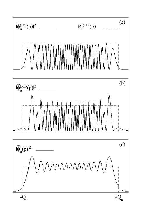
Figure 1: Plots of the classical momentum-space probability distribution, $P_{n}^{(CL)}(p)$ versus $p$, for the quantum bouncer (dashed curve) from Eq. (35) and the corresponding quantum distribution, $|\tilde{\phi}(p)|^{2}$ (solid curves) from Eq. (37c). The imaginary and real parts of $|\tilde{\phi}(p)|^{2}$ from are shown in (a) and (b) and the total $|\tilde{\phi}(p)|^{2}$ in (c). The vertical dashed lines labeled $\pm Q_{n}$ indicate the classical turning points in momentum-space.

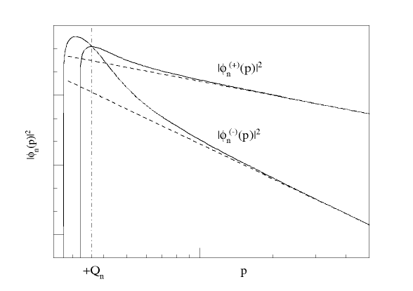
Figure 2: The solid curves show $|\phi(p)|^{2}$ for the symmetric linear potential in Sec. VII obtained by numerical Fourier transform for a typical even ($\phi_{n}^{(+)}(p)$) and odd ($\phi_{n}^{(-)}(p)$) case ($n=11$). The straight dashed lines correspond to the lowest-order non-vanishing predictions in Eqs. (70) and (72). The vertical dot-dash line indicates the classical turning point in momentum-space at $+Q_{n}$ for positive $p$. Note the log-log scales.