ASYMPTOTIC ENERGY PROFILE OF A WAVEPACKET IN DISORDERED CHAINS

Abstract

We investigate the long time behavior of a wavepacket initially localized at a single site $n_{0}$ in translationally invariant harmonic and anharmonic chains with random interactions. In the harmonic case, the energy profile $\overline{\langle e_{n}(t)\rangle}$ averaged on time and disorder decays for large $|n-n_{0}|$ as a power law $\overline{\langle e_{n}(t)\rangle}\approx C|n-n_{0}|^{-\eta}$ where $\eta=5/2$ and $3/2$ for initial displacement and momentum excitations, respectively. The prefactor $C$ depends on the probability distribution of the harmonic coupling constants and diverges in the limit of weak disorder. As a consequence, the moments $\langle m_{\nu}(t)\rangle$ of the energy distribution averaged with respect to disorder diverge in time as $t^{\beta(\nu)}$ for $\nu\geq 2$, where $\beta=\nu+1-\eta$ for $\nu>\eta-1$. Molecular dynamics simulations yield good agreement with these theoretical predictions. Therefore, in this system, the second moment of the wavepacket diverges as a function of time despite the wavepacket is not spreading. Thus, this only criteria often considered earlier as proving the spreading of a wave packet, cannot be considered as sufficient in any model. The anharmonic case is investigated numerically. It is found for intermediate disorder, that the tail of the energy profile becomes very close to those of the harmonic case. For weak and strong disorder, our results suggest that the crossover to the harmonic behavior occurs at much larger $|n-n_{0}|$ and larger time.

I Introduction

There has been large activity for many years in the study of the temporal evolution of an initially localized energy excitation in various nonlinear systems, e.g. the discrete, nonlinear Schrödinger equation (DNLS) Shepelyansky93 ; Molina98 ; Pikovsky08 ; Kopidakis08 , Fermi-Pasta-Ulam (FPU) Bourbonnais90 ; Zavt93 ; Leitner01 ; Snyder06 and Klein-Gordon (KG) model Kopidakis08 ; FLO9 with both uniform and random couplings. In the latter case, the main interest is in the interplay of anharmonicity (nonlinearity) and disorder which is not yet fully understood. For harmonic one-dimensional disordered systems, all eigenmodes (called Anderson modes) of the infinite system are known to be localized and form a complete basis. Then a wave packet at time $t=0$ will remain localized at any time as a linear superposition of Anderson modes of the infinite chain. Whether or not this behavior changes qualitatively by introduction of anharmonicity is highly debated and controversial (see Refs. Pikovsky08 ; Kopidakis08 ; FLO9 and references therein).

Since an analytical treatment of the time evolution of anharmonic systems with disorder is extremely difficult, most investigations have been done by molecular dynamics simulations. In the numerical studies, one typically follows the wavepacket dynamics by monitoring quantities like the participation ratio $P(t)$ (a measure the localization at time $t$), and the time-dependent moments $m_{\nu}(t)$ of the local energy $e_{n}(t)$ (see the definitions below). All this measurements are hampered by statistical errors as well as finite size and finite time effects. Even very long calculation times of, say, 10⁸ microscopic time units (of order picoseconds) may not be entirely conclusive. Indeed, one can never be sure whether the spreading of a wavepacket is complete or only partial in the infinite-time limit. This issues are intimately related to the spontaneous self-trapping of energy (for example in the form of discrete breathers) which is generic in most nonlinear systems.

Independently on complete or incomplete spreading, one might expect that the evolution of the wavepacket tails should yield relevant information on the spreading process itself. In such regions, the typical displacement becomes small enough such that linear approximation of the forces becomes valid. This motivates the investigation of the harmonic chain, as a first necessary step for an insight of the nonlinear case. Despite the apparent simplicity of such a case there are still issues that have not been fully discussed in the literature. Let us briefly review some of the main results known for this case. Without disorder all eigenstates are extended and it is well-known (see e.g. Ref. dk , and references therein) that

$$m_{\nu}(t)\sim t^{\beta(\nu)}\quad$$ (1)

with $\beta(2)=2$, i.e. the energy spreading is ballistic (note that $\nu$ is not necessarily an integer). Introducing disorder and/or anharmonicities, this energy transport is changed and may be superdiffusive ($\beta(2)>1$), diffusive ($\beta(2)=1$) or subdiffusive ($\beta(2)<1$), or it could become logarithmic or disappear ($\beta(2)=0$). If the initial excitation is at site zero with amplitude $u_{0}(0)$, then the disorder averaged propagator $\langle u_{n}(t)\rangle$ is one of the basic quantities. Although $\langle u_{0}(t)\rangle$ for $t\rightarrow\infty$ is known analytically for different classes of disorder ABSO81 , much less is known for $n\neq 0$. Approximating the Anderson modes by plane waves with exponentially decaying amplitudes, it has been shown in Ref. Zavt93 that

$$\langle u_{n}(t)\rangle\equiv\frac{1}{2(\pi\xi_{0}|n|)^{1/2}}\exp[-\frac{(|n|-ct)^{2}}{4\xi_{0}|n|}]$$ (2)

for $|n|\rightarrow\infty$ and $t\rightarrow\infty$. Here, $c$ is the sound velocity and $\xi_{0}$ a measure of the localization length. Eq.(2) shows for $t\rightarrow\infty$ there are two humps which propagate ballistically at the sound velocity $c$, but with an amplitude which decays as $1/\sqrt{t}$. Within its co-moving frame , these humps spread as for normal diffusion. Another approach for calculating $\langle u_{n}(t)\rangle$ is to use a scaling hypothesis ABSO81

$$\langle\tilde{u}_{n}(\omega)\rangle=\langle\tilde{u}_{0}(\omega)\rangle F(n/\xi(\omega))\quad,\quad\omega\rightarrow 0$$ (3)

for the Laplace transform of $\langle u_{n}(t)\rangle)$ for $\omega\rightarrow 0$. A similar Ansatz can be made for $\langle u_{n}(t)\rangle$ AH78 ; AB79 ; RR80 . Here, $\xi(\omega)$ denotes a localization length.

In this paper we investigate the energy profile $\overline{\langle e_{n}(t)\rangle}$ averaged on time and disorder of a wavepacket originating an initially localized excitation. We demonstrate that it asymptotically decays as a power law in space. Thus, the wavepacket remains localized only weakly while its moments appear to diverge in time. This result, which, to the best of our knowledge, has not been reported previously, must be taken into account expecially when attacking more difficult nonlinear case. Indead, some numerical results for the anharmonic chain (a FPU model) will be critically analyzed on the basis of the results on the harmonic one.

The outline of our paper is as follows. In Section II we will introduce the harmonic model, rephrase some of its well-known properties, define the local energy $e_{n}(t)$ and give some information on our numerical approach. A virial theorem for the time averaged local kinetic and potential energy will be proven in Section III. It will be applied in this section for the analytical calculation of the time and disorder average of $e_{n}(t)$. The corresponding analytical result will be compared with the numerical one. Furthermore we will investigate the moments $m_{\nu}(t)$ of the local energy $\langle e_{n}(t)\rangle$. The influence of anharmonicity on $e_{n}(t)$ will be numerically studied in Section IV, and the final Section V contains a summary and some conclusions.

II THE DISORDERED HARMONIC CHAIN

II.1 Property of the Anderson modes

As motivated above we investigate the classical dynamics of a disordered harmonic chain with lattice constant $a$ which is invariant under translations. Its classical Hamiltonian reads:

$$H=\sum\limits_{n}\,\left[\frac{p_{n}^{2}}{2m}+\frac{1}{2}K_{n}(u_{n+1}-u_{n})^{2}\right]\quad.$$ (4)

Here, $u_{n}$ is the displacement of the particle at site $n$, $p_{n}$ the corresponding conjugate momentum, $m$ the particle’s mass, and $K_{n}$ the random coupling constants between nearest neighbors. The $K_{n}$ are independent random variables, identically distributed with some probability distribution $p(K)$. Stability requires all $K_{n}$ to be positive. In our numerical approach, the system is finite with $N$ particles and with free ends, i.e. $K_{\pm N/2}=0$. Otherwise, we shall perform analytical calculations in the thermodynamic limit $N\rightarrow\infty$ where the choice of the boundary conditions does not matter. The equations of motion are

$$m\ddot{u}_{n}=K_{n}(u_{n+1}-u_{n})-K_{n-1}(u_{n}-u_{n-1}).$$ (5)

The general solution of Eqs. (5) with initial conditions $u_{n}(0)=u_{n}$, $\dot{u}_{n}(0)=\dot{u}_{n}$ is given by

$$u_{n}(t)=U_{0}+\dot{U}_{0}t+\upsilon_{n}(t)$$ (6)

where

$$\upsilon_{n}(t)=\sum\limits_{n^{\prime}}\Big{[}u_{n^{\prime}}\Big{(}\sum\limits_{\nu\neq 0}Q^{(\nu)}_{n}Q^{(\nu)}_{n^{\prime}}\cos\omega_{\nu}t\Big{)}+\dot{u}_{n^{\prime}}\Big{(}\sum\limits_{\nu\neq 0}\frac{1}{\omega_{\nu}}Q_{n}^{(\nu)}Q_{n^{\prime}}^{(\nu)}\sin\omega_{\nu}t\Big{)}\Big{]}\quad.$$ (7)

and $U_{0}=\sum\limits_{n}u_{n}/N$, $\dot{U}_{0}=\sum\limits_{n}\dot{u}_{n}/N$ are the position and velocity, respectively, of the center of mass of the whole chain.

The eigenmodes $Q_{n}^{(\nu)}$ with eigenfrequency $\omega_{\nu}$ can be chosen as real with indices $\nu$ in a countable set. They satisfy

$$K_{n}(Q_{n}^{(\nu)}-Q_{n+1}^{(\nu)})+K_{n-1}(Q_{n}^{(\nu)}-Q_{n-1}^{(\nu)})=m\omega_{\nu}^{2}Q_{n}^{(\nu)}.$$ (8)

and they can be normalized, except the uniform eigenmode $Q_{n}^{(0)}\equiv 1$ with $\omega_{0}=0$ which is extended and cannot be normalized for the infinite system. For any size $N$ of a finite system, the translation invariance of the model implies that $\quad Q_{n}^{(0)}=\frac{1}{\sqrt{N}}$ is an eigenmode with eigenfrequency $\omega_{0}=0$. In the limit of an infinite system, all eigenmodes are localized, except this single zero-frequency mode which is extended. However, nothing changes in the problem when choosing the center of mass of the whole system immobile at $U_{0}=0$ with $\dot{U}_{0}=0$. Though the eigenspectrum is discrete for the infinite system, it is dense. The corresponding density of states

$$g(\omega)=\lim\limits_{N\rightarrow\infty}\,\frac{1}{N}\,\sum\limits_{\nu=1}^{N-1}\delta(\omega-\omega_{\nu})$$ (9)

is a smooth function which is known selfav to be self-averaging, i.e. it is independent on the disorder realization with probability one. Moreover, in the small frequency limit, $\omega\to 0$, we have MI70 ; Ishii73

$$g(\omega)\simeq\frac{\sqrt{m\langle K^{-1}\rangle}}{\pi}\quad.\qquad$$ (10)

The localized eigenmodes, decay exponentially with a localization length MI70 ; Ishii73

$$\xi_{\nu}=\xi(\omega_{\nu})\cong\frac{8\langle K^{-1}\rangle/m}{\langle K^{-2}\rangle-\langle K^{-1}\rangle^{2}}\,\omega^{-2}_{\nu}\,a\quad,\quad\omega_{\nu}\rightarrow 0$$ (11)

which diverges at the lower “band” edge at $\omega_{0}=0$.

Then, if the chain is finite with length $L$, there is a frequency $\omega_{L}$ such that the localization length equals the system size, i.e $\xi(\omega_{L})=L=aN$. Consequently, only the eigenmodes with frequency $\omega_{\nu}>\omega_{L}$ can be considered as well localized inside the finite system. while the remaining modes where $\omega_{\nu}<\omega_{L}$ extend over the whole finite system. Their number which is of order of $\sqrt{N}$ goes to infinity in the limit of an infinite system despite their relative weight for $N\rightarrow\infty$ goes to zero as $1/\sqrt{N}$. As a result, they still play a role for transport quantities, like the energy diffusion constant Zavt93 ; DKP89 ; dk or the thermal conductivity LLP03 . Actually, those relatively extended modes behave like acoustic modes whose effective sound velocity is

$$c\;=\;\sqrt{\frac{\langle K^{-1}\rangle^{-1}}{m}}\,\,a$$ (12)

Although these results were originally proven for a chain with mass disorder they also hold for our model. Indeed, letting $y_{n}=({u_{n+1}-u_{n}})/K_{n}$, Eq. (5) is mapped onto the eigenequation with mass disorder. This property has already been used above since the mass average $\langle m\rangle$ has been replaced by $\langle K^{-1}\rangle$.

II.2 Local energy and local virial theorem

We define the local energy:

$$e_{n}(t)=e^{(\rm kin)}_{n}(t)+e^{(\rm pot)}_{n}(t)$$

with kinetic and potential parts

$$e^{(\rm kin)}_{n}(t)=\frac{m}{2}(\dot{u}_{n}(t))^{2}$$ (13)

and

$$e_{n}^{(\rm pot)}(t)= \frac{1}{2}K_{n-1}[u_{n}(t)-u_{n-1}(t)]u_{n}(t)-$$ (14)

$$\frac{1}{2}K_{n}[u_{n+1}(t)-u_{n}(t)]u_{n}(t)$$

respectively. Then, $\sum\limits_{n}\,e^{(\rm pot)}_{n}$ equals the total potential energy in Eq. (4). We will investigate the energy profile for a displacement excitation:

$$u_{n}(0)=A\delta_{n,n_{0}}\quad,\quad p_{n}(0)\equiv 0$$ (15)

and a momentum excitation:

$$u_{n}(0)\equiv 0\quad,\quad p_{n}(0)=B\,\delta_{n,n_{0}}\quad.$$ (16)

For calculating numerically $\{u_{n}(t)\}$ we considered the example of a uniform and uncorrelated distribution of random couplings $K_{n}$ with probability distribution

$$p(K)=\begin{cases}\frac{1}{k(R-1)}&\text{if $k\leq K\leq Rk$,}\\ 0&\text{otherwise.}\end{cases}$$ (17)

where of course $R\geq 1$.

To explore the role of different disorder strengths we fixed $k=1$ and took different $R$. The choice of units is such that $m=1$ and $a=1$. Note that with this particular choices the effective sound velocity, Eq. (12), is $c\;=\;\sqrt{\frac{R-1}{\ln R}}$.

Microcanonical simulations were performed for typically $N=8192$ particles with fourth order symplectic algorithm MA92 , with typical time step $5\times\,10^{-3}$ or less. Although the choice of the initial conditions, Eqs. (15) and  (16), implies $U_{0}=A/N$, $\dot{U}_{0}=0$ and $U_{0}=0$, $\dot{U}_{0}=B/N$, respectively, these nonzero quantities are rather small, since $A$ and $B$ are of order one and $N\gg 1$.

In our numerical experiments, we avoid that the wavepacket reaches the chain boundaries which may generate spurious finite-size effects (reflexions etc.). Thus, one should restrict the maximum simulation time $t_{\rm sim}$ to be smaller than $t_{\rm max}\sim N/c$ where $c$ is the sound velocity.

We also fixed $n_{0}=-N/2+1$ for extending the spatial range of our system, so that one simulates the wavepacket propagation in a semi-infinite medium Snyder06 . Some runs with $n_{0}=0$ where also performed, yielding similar results. Figure 1 shows the numerical profile $e_{n}(t=2000)$ for a momentum excitation with $B=2.0$. The result for a single realization of the disorder exhibits on the log-log-representation strong fluctuations around an average, decaying linearly. Averaging over a large enough number [$\mathcal{O}(10^{3})$] disorder realizations strongly reduces these fluctuations and supports the linear dependence on $|n-n_{0}|$ on the log-log scale. In the next Section we demonstrate that this is indeed the case and compute analytically the exponents associated with such power-lay decay.

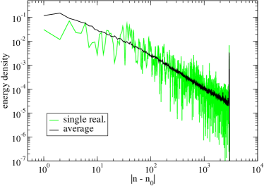
Figure 1: (Color online) Energy profile $e_{n}(t)$ at $t=2000$ for a momentum excitation with $B=2.0$, $N=8192$ particles, $R=4$ and for a single realization of disorder (green line) and averaged over $2\times 10^{3}$ realizations (black line).

The calculation of the time averaged energy profile will be simplified by means of a local virial theorem, that will be proved below. The well-known virial theorem LL82 relates the time average of the total kinetic energy to the time average of the virial. The virial LL82 involves the gradient of the total potential energy. If the potential is harmonic this theorem implies equality between the time averaged total kinetic and total potential energy. In this subsection we will prove that this relationship also holds for the time averaged local kinetic and local potential energy, defined by Eqs. (13) and (14), respectively.

The time average of a function $f(t)$ is defined by

$$\overline{f(t)}=\lim\limits_{T\rightarrow\infty}\frac{1}{T}\int\limits_{0}^{T}\,dt\,f(t)\quad.$$ (18)

Substitution of the general solution $u_{n}(t)$ of Eqs. (6), (7) into Eq. (13) and taking into account

$$\overline{\cos\omega_{\nu}t\cos\omega_{\nu^{\prime}}t}=\frac{1}{2}\,\delta_{\nu\nu^{\prime}}$$

$$\overline{\sin\omega_{\nu}t\sin\omega_{\nu^{\prime}}t}=\frac{1}{2}\,\delta_{\nu\nu^{\prime}}$$

$$\overline{\sin\omega_{\nu}t\cos\omega_{\nu^{\prime}}t}=0\quad.$$ (19)

yields

$$\overline{e_{n}^{(\rm kin)}(t)}=\frac{m}{2}\dot{U}_{0}^{2}+\frac{m}{4}\sum\limits_{\nu\neq 0}(Q^{(\nu)}_{n})^{2}\Big{[}\omega^{2}_{\nu}\Big{(}\sum\limits_{n^{\prime}}u_{n^{\prime}}Q_{n^{\prime}}^{(\nu)}\Big{)}^{2}+\Big{(}\sum\limits_{n^{\prime}}\dot{u}_{n^{\prime}}Q^{(\nu)}_{n^{\prime}}\Big{)}^{2}\Big{]}\quad.$$ (20)

Note that the sum over $\nu$ remains discrete and cannot be replaced by an integral in the limit of an infinite system.

With our definition Eq. (14) of $e_{n}^{(\rm pot)}$, and using Eq. (5), we obtain:

$$e_{n}^{(\rm pot)}(t)=-\frac{m}{2}\ddot{u}_{n}(t)u_{n}(t)\quad.$$ (21)

Substituting $u_{n}(t)$ from Eqs. (6), (7), and since $\upsilon_{n}(t)$ and $\dot{\upsilon}_{n}(t)$ has to remain bounded at all times for any initially localized wavepacket (with finite energy), yields

$$\overline{e_{n}^{(\rm pot)}(t)}=\overline{e_{n}^{(\rm kin)}(t)}\quad,$$ (22)

for all $n$ and arbitrary initial conditions with finite energy in case that the center of mass has been chosen immobile ($\dot{U}_{0}=0$).

III ENERGY PROFILE: HARMONIC CASE

III.1 Energy profile

Without restricting generality we choose $m=1$ and $a=1$. Let us discuss first the case of a displacement excitation for a given disorder realization. In this case, we obtain from Eqs (6) and  (7) for $A=1$ and $U_{0}=0$, $\dot{U}_{0}=0$

$$u_{n}(t) = \sum\limits_{\nu}Q_{n}^{(\nu)}Q_{n_{0}}^{(\nu)}\cos\omega_{\nu}t$$

$$\dot{u}_{n}(t) = -\sum\limits_{\nu\neq 0}\omega_{\nu}Q_{n}^{(\nu)}Q_{n_{0}}^{(\nu)}\sin\omega_{\nu}t$$ (23)

and therefore

$$e^{({\rm kin})}_{n}(t)=\frac{1}{2}\sum\limits_{\nu,\nu^{\prime}\neq 0}\,\omega_{\nu}\omega_{\nu^{\prime}}\,Q^{(\nu)}_{n}Q^{(\nu)}_{n_{0}}Q^{(\nu^{\prime})}_{n}Q^{(\nu^{\prime})}_{n_{0}}\sin\omega_{\nu}t\,\sin\omega_{\nu^{\prime}}t\quad.$$ (24)

Let us discuss first the qualitative $t$-dependence of $e_{n}^{(\rm kin)}(t)$. We will explain how the spectral properties govern its time dependence. Particulary we show that this quantity which is not averaged over time and/or disorder does not decay for $n\rightarrow\infty$ and/or $t\rightarrow\infty$. Since the eigenspectrum of the infinite random system is discrete with a countable basis of localized eigenstates $\{Q^{(\nu)}_{n}\}$, $u_{n}(t)$ has been expanded in this basis (see Eq. (7) and Eq. (III.1)). This expansion is actually an absolutely convergent series of cosine functions of time because

$$|\sum_{\nu}Q_{n_{0}}^{(\nu)}Q_{n}^{(\nu)}|\leq(\sum_{\nu}Q_{n_{0}}^{(\nu)~{}2})^{1/2}(\sum_{\nu}Q_{n}^{(\nu)~{}2})^{1/2}=1$$

Consequently, $u_{n}(t)$ is an almost periodic function in the sense of H. Bohr Bohr . An equivalent definition for such functions is that for any arbitrarily small $\epsilon>0$, there is a monotone sequence of $\tau_{p}$ ($p\in\mathcal{Z}$) (called pseudoperiods) which is relatively dense (that is there exists $L$ such that $\tau_{p+1}-\tau_{p}<L$ for any $p$) and such that for all $p$, $f(t)$ is periodic with period $\tau_{p}$ at the accuracy $\epsilon$ that is $|f(t+\tau_{p})-f(t)|<\epsilon$ for any $p$ and for all $t$. As a consequence of this recurrence property, an almost periodic function cannot go to zero for $t\rightarrow\pm\infty$. The set of almost periodic functions is an algebra, that is linear combinations and products of almost periodic functions are almost periodic functions, as well.

In our case, the set of eigenfrequencies ${\omega_{\nu}}$ is bounded (since the support of the distribution function $p(K)$ is compact) and thus it is straightforward to show that the time derivative $\dot{u}_{n}(t)$ is also an almost periodic function of time, and the local kinetic energy $e^{({\rm kin})}_{n}(t)$ defined by Eq. (13), as well. $e^{({\rm kin})}_{n}(t)$ from Eq. (24) can be decomposed into a time independent term and remaining time dependent terms :

$$e_{n}^{(kin)}(t)=\frac{1}{4}\sum\limits_{\nu\neq 0}\omega_{\nu}^{2}(Q^{(\nu)}_{n}Q^{(\nu)}_{n_{0}})^{2}-\frac{1}{4}\sum\limits_{\nu\neq 0}\omega^{2}_{\nu}(Q^{(\nu)}_{n}Q_{n_{0}}^{(\nu)})^{2}\cos 2\omega_{\nu}t+$$

$$+\frac{1}{4}\sum\limits_{\nu\neq\nu^{\prime}}\omega_{\nu}\omega_{\nu^{\prime}}(Q_{n}^{(\nu)}Q^{(\nu)}_{n_{0}})(Q^{(\nu^{\prime})}_{n}Q^{(\nu^{\prime})}_{n_{0}})[\cos(\omega_{\nu}-\omega_{\nu^{\prime}})t+\cos(\omega_{\nu}+\omega_{\nu^{\prime}})t]\quad.$$ (25)

Note that for a finite chain without disorder,i.e. $K_{n}\equiv K$, the first and second term on the r.h.s of Eq.(III.1) are of order $1/N$ since the eigenmodes are plane waves where $Q_{n}^{(\nu)}\propto 1/\sqrt{N}$. Then $(Q_{n}^{(\nu)}Q_{n_{0}}^{(\nu)})^{2}\propto 1/N^{2}$, and there are only $N$ such terms. Consequently, they will not contribute to $e_{n}^{(\rm kin)}(t)$, in the limit $N\rightarrow\infty$ when the eigenspectrum of the chain becomes absolutely continuous. In that case $e_{n}^{(kin)}(t)$ can be represented by an integral which is a Fourier transform of a smooth function and is obviously not an almost periodic function. It decays to zero at infinite time as expected from ballistic diffusion. This is not true in case of disorder, because each term in the series keeps a non vanishing contribution for the infinite system and $e^{({\rm kin})}_{n}(t)$ does not decay to zero at infinite time because it is almost periodic.

However, in contrast to the ordered chain, $Q_{n}^{(\nu)}Q^{(\nu)}_{n_{0}}$ is not a smooth function of $\omega_{\nu}$, in case of disorder. The reason is that when the eigenspectrum is discrete, arbitrarily small variations of $\omega_{\nu}$ may change the location of the corresponding localized eigenstate by arbitrarily large distances. Thus, these eigenstates $\{Q_{n}^{(\nu)}\}$ are not continuous functions of $\omega_{\nu}$ but depend on the disorder realization as well as $e_{n}^{(\rm kin)}(t)$ and $e_{n}(t)$ (since they are obtained as discrete series explicitly involving these eigenstates). The consequence is that those quantities are not self-averaging, as clearly demonstrated by Fig. 1 for $e_{n}^{(\rm kin)}(t)$.

III.2 Disorder averaged profile

Since $e_{n}^{(kin)}(t)$ is an almost periodic function of time, it is a stationary solution. Its time average drops all cosine terms in Eq. (III.1) and keeps only the constant term, i.e. we get

$$\overline{e_{n}^{(kin)}(t)}=\frac{1}{4}\sum\limits_{\nu\neq 0}\omega_{\nu}^{2}(Q^{(\nu)}_{n}Q^{(\nu)}_{n_{0}})^{2}.$$

An attempt to justify the use of the time averaged quantity will be given below. $\overline{e_{n}^{(kin)}(t)}$ and $\overline{e_{n}(t)}$ still depend on the disorder realization. Therefore it is reasonable to calculate the corresponding disorder averaged quantities, as well. Despite they cannot be observed for any single disorder realization, they give information on the general behavior of the profiles. Then we arrive at

$$\langle\overline{e_{n}^{(\rm kin)}(t)}\rangle=\frac{1}{4}\langle\sum\limits_{\nu\neq 0}\omega^{2}_{\nu}(Q^{(\nu)}_{n}Q^{(\nu)}_{n_{0}})^{2}\rangle$$ (26)

for the infinite system.

Note that, in the infinite system, the set of eigenvalues and eigenvectors are discontinuous functions of the disorder realization. Yet, according to Wegner Wegner75 , the disorder average $\langle F(\{Q^{(\omega)}_{n}\})\rangle$ of an arbitrary function $F(\{Q^{(\nu)}_{n})\})$ of the eigenvectors can be well defined as a smooth function of $\omega$ as a limit for finite systems with size $N\rightarrow\infty$

$$\langle F(\{Q^{(\omega)}_{n})\})\rangle g(\omega)\delta\omega=\lim_{N\rightarrow+\infty}\int\left(\frac{1}{N}\sum_{\omega<\omega_{\nu}<\omega+\delta\omega}F(\{Q^{(\nu)}_{n}\})\right)\prod_{n=1}^{N}p(K_{n})dK_{n}$$

The sum in the integral is restricted to eigenvalues $\omega_{\nu}$ which belong to an interval $[\omega,\omega+\delta\omega]$ of small width $\delta\omega$ and $g(\omega)$ is the density of states defined by Eq. (9).

Then, we obtain from Eq. (26) :

$$\langle\overline{e_{n}^{(\rm kin)}(t)}\rangle=\frac{1}{4}\int\limits_{0}^{\infty}d\omega\omega^{2}g(\omega)\lim\limits_{N\rightarrow\infty}(N\langle(Q_{n}^{(\omega)}Q^{(\omega)}_{n_{0}})^{2}\rangle)\quad.$$ (27)

Since $\overline{e_{n}^{(\rm pot)}(t)}=\overline{e_{n}^{(\rm kin)}(t)}$, for $N=\infty$ and all realizations of $\{K_{n}\}$ the time and disorder averaged energy profile is given by

$$\langle\overline{e_{n}(t)}\rangle=2\langle\overline{e_{n}^{(\rm kin)}(t)}\rangle\quad,$$ (28)

i.e. the calculation of $\langle\overline{e_{n}(t)}\rangle$ is reduced to that of $g(\omega)$ and the “quadratic” correlation function $\langle(Q^{(\omega)}_{n}Q^{(\omega)}_{n_{0}})^{2}\rangle$ for $N\rightarrow\infty$. $\{Q^{(\omega)}_{n}\}$ is the solution of the eigenvalue equation (8) with $\omega_{\nu}$ replaced by $\omega$.

Before we come to the evaluation of the “quadratic” correlation function, let us return to Eq.(III.1). Making again use of the self-averaging of the density of states we obtain for the second term on its r.h.s.:

$$-\frac{1}{4}\int\limits_{0}^{\infty}d\omega\,\omega^{2}g(\omega)\lim\limits_{N\rightarrow\infty}(N\langle(Q_{n}^{(\omega)}Q^{(\omega)}_{n_{0}})^{2}\rangle)\cos 2\omega t\quad.$$

Below, it will be shown that $\lim\limits_{N\rightarrow\infty}(N\langle(Q^{(\omega)}_{n}Q_{n_{0}}^{(\omega)})^{2}\rangle)$ is a finite and smooth function of $\omega$. Therefore, the disorder averaged second term will converge to zero, for $t\rightarrow\infty$, due to $g(\omega)\rightarrow g_{0}={\rm const.},$ for $\omega\rightarrow 0$. The same property should hold for the disorder average of the square bracket term in Eq. (III.1). With the density of states $g(\omega,\omega^{\prime})$ giving the joint distribution for two eigenfrequencies the disorder averaged square bracket term becomes a double integral over $\omega$ and $\omega^{\prime}$. Although we do not have a rigorous proof, $\lim\limits_{N\rightarrow\infty}(N^{2}\langle(Q_{n}^{(\omega)}Q^{(\omega)}_{n_{0}})(Q^{(\omega^{\prime})}_{n}Q_{n_{0}}^{(\omega^{\prime})})\rangle)$ which is part of the integrand should be a finite and smooth function of $\omega$ and $\omega^{\prime}$. Then, taking the limit $N\rightarrow\infty$ first, the square bracket term should converge to zero for $t\rightarrow\infty$. If this is true the disorder averaged energy profile converges to an asymptotic profile for $t\rightarrow\infty$ which is consistent with our numerical result. Indeed, the disorder averaged profile in Fig. 1 depends on $t$ only very weakly, for large $t$. In that case the asymptotic profile equals the time averaged one.

Now we come back to the “quadratic” correlation function. Due to the disorder average it will depend only on $|n-n_{0}|$. Since the Anderson modes are exponentially localized one expects that this correlation function decays exponentially with $|n-n_{0}|$. To prove this we first present a crude heuristic approach by assuming

$$Q_{n}^{(\nu)}\approx\mathcal{N}_{\nu}\exp\left(-\frac{|n-n_{\nu}|}{\xi_{\nu}}\right)$$ (29)

where the “center of mass” of the Anderson mode $\nu$ is at $n_{\nu}$, which is a random variable, depending on $\{K_{n}\}$. $\mathcal{N}_{\nu}$ is a normalization constant. It should be remarked, that the envelope of an Anderson mode $Q^{(\nu)}_{n}$ decays exponentially, but not $Q^{(\nu)}_{n}$ itself. Therefore Eq. (29) is a crude approximation neglecting sign changes of $Q^{(\nu)}_{n}$ with $n$. Substituting $Q_{n}^{(\nu)}$ from Eq.(29) into the “quadratic” correlation function and using :

$$\langle f(n_{\nu})\rangle\approx\frac{1}{N}\sum\limits_{n_{\nu}=1}^{N}f(n_{\nu})\quad,$$ (30)

we get :

$$\langle(Q_{n}^{(\nu)}Q^{(\nu)}_{n_{0}})^{2}\rangle\approx\frac{1}{N}\mathcal{N}_{\nu}^{4}[\coth\frac{2}{\xi_{\nu}}+|n-n_{0}|]\exp[-\frac{2}{\xi_{\nu}}|n-n_{0}|]$$ (31)

i.e. the “quadratic” correlation function decays exponentially.

For an analytical calculation of the “quadratic” correlation function in Eq.(27) one can use the approach presented in Refs. Wegner75 ; Wegner81 ; Wegner85 . These authors prove that the computation of the correlation functions $\langle Q^{(\omega)}_{n}Q^{(\omega)}_{n_{0}}\rangle$ and $\langle|Q^{(\omega)}_{n}||Q^{(\omega)}_{n_{0}}|\rangle$ for $|n-n_{0}|\rightarrow\infty$ is reduced to the solution of an eigenvalue problem for an integral kernel. As a result, these correlation functions decay exponentially for large $|n-n_{0}|$ with an inverse localization length given by $-\ln|\lambda_{max}(\omega)|$. $|\lambda_{max}(\omega)|$ is the largest absolute value of the eigenvalues of the kernel. It is smaller than one. Applying that approach it follows for $|n-n_{0}|\rightarrow\infty$

$$\langle(Q^{(\omega)}_{n}Q^{(\omega)}_{n_{0}})^{2}\rangle\cong\alpha(\omega)\exp(-|n-n_{0}|/\xi_{2}(\omega))$$ (32)

with a correlation length $\xi_{2}(\omega)$. We note that the eigenvalue problem in form of an integral equation can only be used to calculate correlation functions of the Anderson modes and not directly to compute the energy profile itself. But the former is needed (see Eq. (27)) for the latter.

The correlation lengths (localization lengths) of the correlation functions calculated in Refs. Wegner75 ; Wegner81 ; Wegner85 and of the “quadratic” correlation function Eq. (32) are different from each other and different from $\xi(\omega)$ (Eq. (11)), for finite $\omega$. But for $\omega\rightarrow 0$ they exhibit the same divergence, i.e. it is (see Eq. (11)):

$$\xi_{2}(\omega)\cong c_{2}\omega^{-2}\quad,\quad\omega\rightarrow 0$$ (33)

with a positive constant $c_{2}$, depending on $p(K)$.

The pre-exponential factor $\alpha(\omega)$ can be determined as follows. Assuming that Eq. (32) is valid for all $|n-n_{0}|$, summation of the l.h.s. and r.h.s. of that equation and accounting for the normalization $\sum\limits_{n}(Q^{(\omega)}_{n})^{2}=1$ for $\omega=\omega_{\nu}$ (remember that $Q^{(\nu)}_{n}$ has been chosen as real) yields for $N\rightarrow\infty$:

$$\alpha(\omega) \cong \frac{1}{N\coth(1/\xi_{2}(\omega))}$$ (34)

$$\cong \frac{\omega^{2}}{Nc_{2}}\quad,\quad\omega\rightarrow 0\quad.$$

In the last line, Eq. (33) has been applied. With Eqs.  (32), (34) and (27), it follows from Eq. (28):

$$\langle\overline{e_{n}(t)}\rangle\cong\frac{1}{2}\int\limits_{0}^{\infty}d\omega\;g(\omega)\omega^{2}\frac{\exp(-|n-n_{0}|/\xi_{2}(\omega))}{\coth(1/\xi_{2}(\omega))}\quad.$$ (35)

The asymptotic $|n-n_{0}|$-dependence is governed by the small-$\omega$ behavior of the integrand. From Eq. (10) we get

$$g(\omega)=dI(\omega)/d\omega\cong\sqrt{\langle K^{-1}\rangle}/\pi\quad,\quad\omega\rightarrow 0\;.$$ (36)

Assuming that Eqs. (33) and (36) are valid for all $\omega$ will not influence the asymptotic dependence of $\langle\overline{e_{n}(t)}\rangle$ on $|n-n_{0}|$. Then we get from Eq. (35) for the infinite chain and a displacement excitation:

$$\langle\overline{e_{n}(t)}\rangle\cong\frac{3}{16}\sqrt{c_{2}^{3}\langle K^{-1}\rangle/\pi}\,\,\,|n-n_{0}|^{-5/2},\,\,\,|n-n_{0}|\rightarrow\infty,$$ (37)

i.e. the time and disorder averaged energy profile decays as a power law in $|n-n_{0}|$ with an exponent $\eta=5/2$.

So far we have discussed the energy profile for a displacement excitation. The corresponding calculation for a momentum excitation is similar. With the initial condition Eq. (16) and $B=1$, Eq. (7)leads to

$$\dot{u}_{n}(t)=\sum\limits_{\nu=1}^{N-1}Q_{n}^{(\nu)}Q_{n_{0}}^{(\nu)}\cos\omega_{\nu}t\quad\quad.$$ (38)

Besides $\cos\omega_{\nu}t$ the main difference to $\dot{u}_{n}(t)$ for a displacement excitation (see Eq. (III.1)) is the absence of the prefactor $\omega_{\nu}$ of $Q_{n}^{(\nu)}Q_{n_{0}}^{(\nu)}$. As a consequence one obtains

$$\langle\overline{e_{n}(t)}\rangle\cong\frac{1}{2}\int\limits_{0}^{\infty}d\omega g(\omega)\frac{\exp(-|n-n_{0}|/\xi_{2}(\omega))}{\coth(1/\xi_{2}(\omega))}$$ (39)

where $\omega^{2}$ in Eq. (35) is replaced by one. With the same assumptions as above we obtain for the infinite chain and a momentum excitation:

$$\langle\overline{e_{n}(t)}\rangle\cong\frac{1}{8}\sqrt{c_{2}\langle K^{-1}\rangle/\pi}\,\,\,|n-n_{0}|^{-3/2},\quad\quad|n-n_{0}|\rightarrow\infty\quad.$$ (40)

It is not surprising that we find a power law decay again. The corresponding exponent is $\eta=3/2$.

Figures 2 and 3 report the numerical result for the disorder averaged energy profile at different large times of a displacement and momentum excitation, respectively. They clearly demonstrate first that, the numerical result of the disorder averaged energy profile becomes independent of $t$ for $t$ large enough, and second, that it converges to a power law for large $|n-n_{0}|$ with exponents predicted by the analytical calculation. The three spikes at the $t$-dependent positions $n(t)$ are the phonon fronts propagating with the effective sound velocity, Eq. (12).

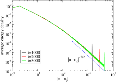
Figure 2: (Color online) Energy profile at three different times averaged over 10³ realizations of the disorder with $R=4$ for $N=8192$ particles and a displacent excitation with $A=2$. The dashed line is the predicted power law decay, Eq. (37). The ballistic peaks propagate at a velocity $c=1.476$ in agreement with the value $c=1.471...$ computed from Eq. (12).

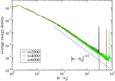
Figure 3: (Color online) Same as Fig. 2 but for a momentum excitation with $B=2$ and averaged over $2\times 10^{3}$ realizations. The dashed line is the predicted power law, Eq. (40).

There is a finite size effect for $N<\infty$, due to the existence of extended states. For $\omega\lesssim\omega_{L}=\theta/\sqrt{N}$, (with $\theta$ being a suitable constant $\mathcal{O}(1)$), it is:

$$\langle(Q_{n}^{(\omega)}Q_{n_{0}}^{(\omega)})^{2}\rangle\approx\frac{4}{N}\sin^{2}(cqn)\sin^{2}(cqn_{0})$$ (41)

where $\omega\cong cq$. With $g(\omega)\approx g_{0}$ for the density of extended states it is easy to estimate the contribution of those to $\langle\overline{e_{n}(t)}\rangle$ in case of a displacement excitation:

$$\langle\overline{e_{n}(t)}\rangle^{(\textrm{ext})}\approx\frac{\theta^{3}g_{0}}{6}N^{-5/2}\quad\quad.$$ (42)

If $1\ll|n-n_{0}|\ll N$, then it is $\langle\overline{e_{n}(t)}\rangle=\langle\overline{e_{n}(t)}\rangle^{(\textrm{loc})}+\langle\overline{e_{n}(t)}\rangle^{(\textrm{ext})}\cong\langle\overline{e_{n}(t)}\rangle^{(\textrm{loc})}\sim|n-n_{0}|^{-5/2}$. For $|n-n_{0}|<N$ but $|n-n_{0}|=\mathcal{O}(N)$ there is a crossover value $|n-n_{0}|_{c.o.}$ depending on $\theta,g_{0}$ etc. such that

$$\langle\overline{e_{n}(t)}\rangle^{(\rm loc)}\cong\langle\overline{e_{n}(t)}\rangle^{{(\textrm{ext})}}\sim N^{-5/2}\quad\quad.$$ (43)

For $N=8192$ this contribution is of order 10^-10. The corresponding contribution for a momentum excitation is

$$\langle\overline{e_{n}(t)}\rangle^{(\textrm{ext})}\sim N^{-3/2}\quad,$$ (44)

being of order 10^-6 for $N=8192$.

Figure 4 compares the energy profiles for different strengths of the disorder, i.e. for various values of the parameter $R$. We limited ourselves to the case of a displacement excitation. The profiles display the same decay law. The cases with stronger disorder attain the asymptotic profile at smaller distances since in this case the localization lengths are shorter. As seen from Figure 4, the data are consistent with the expectation that the asymptotic profile is reached for $|n-n_{0}|\gg\xi_{\textrm{min}}$. The values of $\xi_{\textrm{min}}$ given in that figure are a rough estimate of the shortest localization length obtained by extrapolating the formula (11) at $\omega=\omega_{max}=2c$, i.e. $\xi_{min}=\xi(\omega_{max})$.

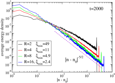
Figure 4: (Color online) Disorder averaged energy profiles at $t=2000$ for a displacement excitation with $A=2$ and increasing disorder strengths (top to bottom). Other parameters as in Fig.1. The dashed line indicates the predicted power law Eq. (37)

The prefactor of both power laws, Eqs. (37) and (40) depends on the disorder as demonstrated by Figure 4. It seems reasonable that $\xi_{2}\cong\lambda\xi(\omega)$ for $\omega\rightarrow 0$ with a positive parameter $\lambda$, independent on $\omega$ and the disorder. Eqs. (11) and (33), together with this hypothesis, imply:

$$c_{2}=8\lambda\frac{\langle K^{-1}\rangle}{\langle K^{-2}\rangle-\langle K^{-1}\rangle^{2}}\quad.$$ (45)

Again $m=1$ and $a=1$ has been used. For the uniform distribution $p(K)$, Eq. (17), $\langle K^{-1}\rangle$ and $\langle K^{-2}\rangle$ can easily be calculated. From this we obtain:

$$c_{2}(R)=8\lambda\frac{(R-1)R\ln R}{(R-1)^{2}-R(\ln R)^{2}}$$

$$\cong 72\lambda(R-1)^{-2}[1+\mathcal{O}(R-1)]$$ (46)

Note, that $c_{2}(R)$ diverges in the no-disorder-limit $R\rightarrow 1^{+}$, as it should be since only extended states exist thereby. Accordingly, $\xi(\omega)$ should become infinite for all $\omega$.

Introducing $c_{2}(R)$ from the first line of Eq. (III.2) and $\langle K^{-1}\rangle(R)=(\ln R)/(R-1)$ into the prefactor $C(R)$ of the power laws, Eqs. (37) and (40), leads to the $R$-dependence shown in Fig. 5 in case of a displacement and a momentum excitation, respectively. The unknown parameter $\lambda$ has been adjusted in order to fit the numerical result for the prefactors. The latter are obtained from the numerical data in Figures 2 and 3 extrapolating $\langle e_{n}(t)\rangle|n-n_{0}|^{\eta}$ at large $|n-n_{0}|$.

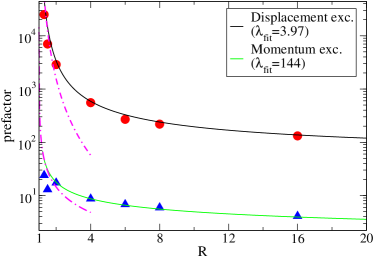
Figure 5: (Color online) Dependence of the prefactors $C(R)$ on the disorder strength $R$ for a displacement ($A=2$) and momentum ($B=2$) excitation: numerical (full circles and triangles respectively) and analytical result Eqs. (37), (40) with formula (III.2) (solid lines). Dash-dotted lines are the expected asymptotic behaviors for $R\to 1^{+}$, $(R-1)^{-3}$ and $(R-1)^{-1}$, respectively. The fitting parameter $\lambda_{\rm fit}$ is given in the legend.

The numerical and analytical result for the prefactor in case of a displacement excitation agree satisfactorily, even for the smallest value of $R=1.3$. Investigating the profile for even smaller values is hampered for our finite chain by the increase of the localization length with decreasing $(R-1)$. The same agreement is also valid in case of the momentum excitation, except for the two smallest $R$-values at 1.3 and 1.5. Eq. (7) demonstrates that the weight of the low-lying Anderson modes for a momentum excitation is by a factor $1/\omega_{\nu}$ higher than for a displacement excitation. Since the localization length increases with decreasing $\omega_{\nu}$, this could be the reason for the “asymmetric” behavior of $C(R)$ for both kind of excitations. Indeed, we have observed that $\langle e_{n}(t)\rangle|n-n_{0}|^{3/2}$ does not reach a stationary value, for e.g. $R=1.3$. The strong deviation of the fit parameter $\lambda$ for the displacement and momentum excitation may originate also from this fact.

III.3 Moments of the local energy

A customary way to describe wavepacket diffusion is to look at time evolution of moments of the energy distribution that are defined as

$$m_{\nu}(t)\;=\;\frac{\sum_{n}\,|n-n_{0}|^{\nu}e_{n}(t)}{\sum_{n}\,e_{n}}$$ (47)

(the denominator is clearly only a scale factor). Of particular interest for a statistical characterization are the disorder averaged moments $\langle m_{\nu}(t)\rangle$. Their numerical result is shown in Figure 6. If one uses the asymptotics Eqs. (37), (40) and introduces a cutoff of the sum in the numerator of Eq. (47) at the ballistic distance $|n-n_{0}|=ct$ one obtains

$$\langle m_{\nu}(t)\rangle\;\propto\;t^{\beta(\nu)},\quad\beta(\nu)\;=\;\left\{\begin{array}[]{ll}\nu+1-\eta&,\quad\nu>\eta-1\\ 0&,\quad\nu<\eta-1\quad.\end{array}\right.$$ (48)

For $\nu=\eta-1$ there is a logarithmic divergence of $\langle m_{\nu}(t)\rangle$ with time. As demonstrated in Fig. 7, the numerical values of $\beta(\nu)$ are in excellent agreement with Eq. (48). This also implies that the contribution of the traveling peaks is not relevant as implicitly assumed in the derivation of Eq. (48).

This result is consistent with the values that could be inferred by Datta and Kundu dk . Indeed, they predict $\beta(2)=1/2$ and $\beta(2)=3/2$, respectively, for a displacement and momentum excitation. Notice that, if one looks only at $m_{2}(t)$ one would incorrectly conclude that the two cases would correspond to sub- and superdiffusive behavior respectively. A full analysis of the spectrum of moments and of the wavefront shape is necessary to assess the real nature of dynamics.

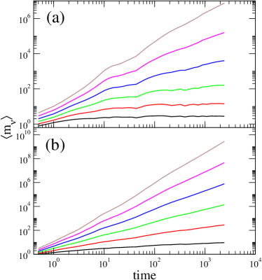
Figure 6: (Color online) Evolution of moments $\langle m_{\nu}(t)\rangle$ for $\nu=0.5,1,1.5,2,2.5,3$ (bottom to top respectively) for the harmonic chain $N=8192$, $R=6$. Displacement (a) and momentum (b) excitation ($A=2$ and $B=2$ respectively). Averages are over $6\times 10^{3}$ disorder realizations.

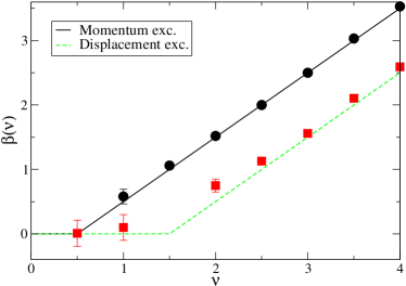
Figure 7: (Color online) Comparison between the exponents measured numerically for momentum and displacement excitations (full circles and squares respectively) and the analytical result Eq. (48), same parameters as in Fig. 6. The exponents are evaluated by a power-law fit. Error bars are estimated from the fluctuations of the (discrete) logarithmic derivative ${\Delta\log\langle m_{\nu}(t)\rangle}/{\Delta\log t}$ and are reported only when larger than symbols’ size.

IV ENERGY PROFILE: ANHARMONIC CASE

In this section we will investigate numerically the $n$-dependence of the energy profile averaged over the disorder in the presence of anharmonicity. Particularly, we will check whether its tails can be described by those of the harmonic chain. As a model we have chosen the Fermi-Pasta-Ulam (FPU) chain with cubic nonlinear force

$$m\ddot{u}_{n} = K_{n}(u_{n+1}-u_{n})-K_{n-1}(u_{n}-u_{n-1})$$ (49)

$$+G(u_{n+1}-u_{n})^{3}-G(u_{n-1}-u_{n})^{3}.$$

It reduces to the harmonic chain for $G=0$. For simplicity, we considered the case of uniform nonlinear coupling $G$ ($G=1$ in the following).

The analysis of the previous section shows that the behavior of the harmonic chain follows all the expected features. Which influence of the anharmonicity do we expect? If the initially localized energy would spread completely it would be $e_{n}(t),\longrightarrow 0$ for $t\rightarrow\infty$, for all $n$. For incomplete spreading, however, $\langle e_{n}(t)\rangle$ for $t$ large enough should decay by the power laws Eqs. (37) or Eqs. (40), again, and the amplitudes of oscillations at sites far away from site $n_{0}$ of the initial excitation should become so small that the harmonic approximation applied to those tails should become valid.

A detailed analysis of the effects of nonlinearity goes beyond the scope of the present work. We thus limited ourselves to the case of FPU with initial displacement excitation with $A=2$. We checked that the energy is about a factor of 2 larger with respect to the $G=0$ case meaning that the nonlinear part of the potential is sizeable. We considered the usual definition of $e^{(\rm pot)}_{n}$ where $K_{i}[u_{i+1}-u_{i}],$ $i=n-1,n$ in Eq. (14) is replaced by $V^{\prime}_{i}(u_{i+1}-u_{i})$ with $V_{i}(x)=K_{i}x^{2}/2+Gx^{4}/4$. As for the harmonic case, we performed the average over disorder at three different times.

The average energy profiles for three different disorder strengths are reported in Fig. 8. The profiles still show a pretty slow decay, reminiscent of the harmonic case. From Fig. 8 we first observe that the convergence of $\langle e_{n}(t)\rangle$ to a limiting profile at $t=\infty$ becomes slower for larger disorder strength $R$, i.e. for shorter localization lengths. Second, whereas the profile for $R=4$ and the largest time $t=6000$ can be satisfactorily fitted by the power law Eq. (37), this is less obvious for $R=2$ and $R=8$. For $R=2$ and $|n-n_{0}|>1000$ the profile is practically time independent for $t\geq 2000$. But in contrast to the harmonic case (see Fig. 2) it does not reveal the asymptotic power law $|n-n_{0}|^{-5/2}$, although the data suggest that this may happen for $|n-n_{0}|\geq 3000$. For $R=8$ the profile follows that power law for $100<|n-n_{0}|<1000$, i.e. for about a decade, but deviates for $|n-n_{0}|>1000$. However, comparing this profile for the three different values for $t$ hints that the range of the power law decay may increase with increasing $t$. In addition, the profiles display some form of weak ”broadening” of the tails indicating that some energy is indeed slowly propagating.

As a consequence, the disorder averaged moments $\langle m_{\nu}(t)\rangle$ do not display a convincing scaling with time. Even for statistically accurate data as the one in Fig. 8, the effective exponents (as measured for example by the logarithmic derivatives of $\langle m_{\nu}(t)\rangle$) display sizeable oscillations which are well outside the range of the statistical fluctuations (see Fig. 9). Similar results are obtained for momenta of different order (not reported).

We may thus argue that, at least in the considered parameter range, the nonlinear case has a core which remain almost localized (in a similar way as the harmonic case) but in addition there must be a small propagating component. The fraction of such propagating component increases upon increasing the energy and/or nonlinearity. As a consequence, with the data at hand it is impossible to draw definite conclusions on the nature of the spreading process.

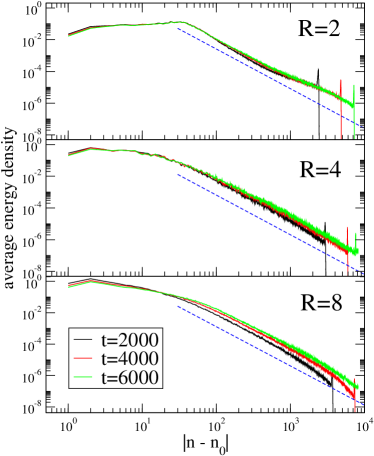
Figure 8: (Color online) FPU model: Disordered-average energy profile at three different times averaged over $10^{3}$ realizations of the disorder and for different disorder strengths $R$. Chain of $N=8192$ particles with displacement excitation $A=2$. For comparison, the predicted power law decay for the harmonic chain, Eq. (37), is also drawn (dashed lines).

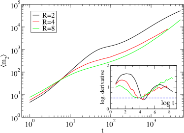
Figure 9: (Color online) FPU model: Evolution of $\langle m_{2}(t)\rangle$ for $R=2,4,8$ (top to bottom respectively) same parameters as in Fig. 8. The inset reports the (discrete) logarithmic derivative ${\Delta\log\langle m_{2}(t)\rangle}/{\Delta\log t}$ of the data versus $\log t$. For comparison, the value for the harmonic chain $\beta(2)=1/2$ is also drawn (dashed horizontal line).

V SUMMARY AND CONCLUSIONS

The relaxation of an initially localized excitation in a translationally invariant chain of particles has been studied for harmonic and anharmonic nearest neighbor couplings. The main focus has been on the energy profile $\langle e_{n}(t)\rangle$, the moments $\langle m_{\nu}(t)\rangle$, both averaged over the disorder, and the relation between the asymptotic $t$-dependence of $\langle m_{\nu}(t)\rangle$ with the asymptotic $n$-dependence of $\langle\overline{e_{n}(t)}\rangle$. As far as we know, this has neither been explored for the anharmonic nor for the harmonic case due to the lack of analytical knowledge of $\langle\overline{e_{n}(t)}\rangle$ for $|n-n_{0}|\rightarrow\infty$.

For the harmonic model we succeeded to determine analytically the disorder and time averaged energy profile $\langle\overline{e_{n}(t)}\rangle$ for a displacement and a momentum excitation at site $n_{0}$ and initial time $t=0$. Whereas $e_{n}(t)$ is a quasiperiodic function which does not converge for $t\rightarrow\infty$ we have argued that $\langle e_{n}(t)\rangle$ converges for $t\rightarrow\infty$. In that case $\langle\overline{e_{n}(t)}\rangle$ gives the limiting profile averaged over the disorder. The analytical calculation yields a power law decay

$$\langle\overline{e_{n}(t)}\rangle\cong C(R)|n-n_{0}|^{-\eta}$$ (50)

for $1\ll|n-n_{0}|\ll N$, in case the system is finite. The exponent $\eta$ and the prefactor $C(R)$ depend on the type of excitation. For a displacement and momentum excitation we have found $\eta=5/2$ and $\eta=3/2$, respectively, in good agreement with the numerical values. This agreement also holds for the analytical and numerical results for the $R$-dependence of $C(R)$, except for the two smallest values of $R$ in case of a momentum excitation. Accordingly our assumption $\xi_{2}(\omega)\sim\xi(\omega)$ for $\omega\rightarrow 0$ is supported. From this proportionality it also follows that $C(R)$ diverges at $R=1$, the no-disorder limit. The power law decay, Eq. (50), originates from the gapless excitation spectrum of the Anderson modes. It is the consequence of the translational invariance of model  (4). Destruction of this invariance by adding, e.g. an on-site potential like in the KG model generates an energy gap. The corresponding localization length at the lowest eigenfrequency will not diverge anymore, and therefore the energy profile will decay exponentially for $|n-n_{0}|\rightarrow\infty$. However, we stress that any lattice model without an external potential has to be invariant under arbitrary translations. This implies a gapless spectrum which is the origin of the power law decay of the profile.

The power law decay of $\langle\overline{e_{n}(t)}$ has remarkable consequences on the asymptotic $t$-dependence of the moments. If we use Eq. (50) to calculate the time and disorder averaged $\nu$-th moment we get for displacement and momentum excitation:

$$\langle\overline{m_{\nu}(t)}\rangle=\infty$$ (51)

for all $\nu\geq 2$; note that, for instance, $\langle\overline{m_{1}(t)}\rangle$ is finite for a displacement, but not for a momentum excitation. The result, Eq. (51), implies that the disorder averaged moment $\langle m_{\nu}(t)\rangle$ must diverge with time, although the initial local energy excitation does not spread completely. This power law divergence of $\langle m_{\nu}(t)\rangle$ with time is clearly supported by the numerical result for $\nu\geq 2$ and $\nu\geq 1$ for the displacement and momentum excitation, respectively. As a matter of fact, consideration of $m_{2}(t)$ alone is not sufficient to conclude that the energy diffuses. This is one of the main messages of the paper.

The analytically exact result for $\langle\overline{e_{n}(t)}\rangle$ in case of harmonic interactions also allows to check how far the tails of an anharmonic chain, where the average displacements become arbitrary small, can be described by the tails of the harmonic system Although no definite conclusion can be drawn, we have found evidence for a crossover of the energy profile of the anharmonic to that of the harmonic chain. However, for the weakest and strongest strength of disorder this crossover seems to occur for $|n-n_{0}|>3000$ and for $t>6000$, respectively. This may be explained as follows. The localization length $\xi_{2}(\omega)$ is large for weak disorder. Since $|n-n_{0}|/\xi_{2}(\omega)$ enters into the calculation of the disorder averaged profile (see Eq. (35)) the asymptotic power laws, Eqs. (37) and  (40), occur at larger values of $|n-n_{0}|$. For large disorder, $\xi_{2}(\omega)$ is small. But the time scale for tunneling processes responsible for the energy propagation increases significantly due to an increase of the potential barriers. Therefore the convergence to a limiting profile is much slower which is exactly what we observed (see Fig. 7). The increase of the localization length for weak disorder and the increase of the relevant time scale of the relaxation for strong disorder probably are also the reasons for the absence of a convincing scaling of the moments $\langle m_{\nu}(t)\rangle$. In order to test this, one has to increase both, the number of particles and the simulation time significantly. Requiring a similar good statistic of the data this has not been possible so far within the available CPU time. If it is true that the asymptotic energy profile agrees with that of the harmonic chain this would imply that the moments $\langle m_{\nu}(t)\rangle$ for the anharmonic model for $\nu\geq 2$ diverge with time, as well, although the energy does not spread completely.

From our results, it is nonetheless clear that the interplay of localized and almost-extended modes leads to a nontrivial decay of wavepackets amplitudes and this must be taken into account when dealing with the nonlinear case.

- (1) D.L. Shepelyansky, Phys. Rev. Lett., 70 , 1787 (1993).
- (2) M.I. Molina, Phys. Rev. B 58 12547 (1998).
- (3) A. S. Pikovsky and D. L. Shepelyansky, Phys. Rev. Lett. 100 094101 (2008).
- (4) G. Kopidakis, S. Komineas, S. Flach, and S. Aubry, Phys. Rev. Lett. 100 084103 (2008).
- (5) R. Bourbonnais and R. Maynard, Phys. Rev. Lett., 64 1397 (1990).
- (6) G. S. Zavt, M. Wagner, A. Lütze, Phys. Rev. E 47 4108 (1993).
- (7) D.M. Leitner, Phys. Rev. B 64, 94201 (2001).
- (8) K.A. Snyder, T.R. Kirkpatrick, Phys. Rev. B 73 134204 (2006).
- (9) S. Flach, D.O. Krimer, and Ch. Skokos, Phys. Rev. Lett. 102, 024101 (2009).
- (10) P.K. Datta, K. Kundu, Phys. Rev. B 51, 6287 (1995).
- (11) S. Alexander, J. Bernasconi, W.R. Schneider, and R. Orbach, Rev. Mod. Phys., 53, 175 (1981).
- (12) S. Alexander and T. Holstein, Phys. Rev. B 108, 301 (1978).
- (13) S. Alexander and J. Bernasconi, J. Phys. C12, L1, (1979)
- (14) P.M. Richards and R.L. Renken, Phys. Rev. B21, 3740 (1980)
- (15) T. Burke and J.L. Lebowitz, J. Math. Phys. 9, 1526 (1968)
- (16) H. Matsuda and K. Ishii, Suppl. Prog. Phys. 45, 56 (1970)
- (17) K. Ishii, Suppl. Prog. Theor. Phys. 53, 77 (1973)
- (18) D. H. Dunlap, K. Kundu and P. Phillips, Phys. Rev. B 40, 10999 (1989)
- (19) S. Lepri, R. Livi, and A. Politi, Phys. Rep. 377, 1 (2003).
- (20) R.I. McLachlan and P. Atela, Nonlinearity 5, 541 (1992).
- (21) L.D. Landau and E.M. Lifshitz, Mechanics I (Butterworth Heinemann, Oxford, 1982)
- (22) F. Wegner, Z. Phys. B22, 273 (1975).
- (23) M. Kappus and F. Wegner, Z. Phys. B45, 15 (1981)
- (24) A. Mielke and F. Wegner, Z. Phys. B62, 1 (1985).
- (25) E.A. Bredikhina Almost Periodic Functions in M. Hazewinkel (ed.) Encyclopedia of Mathematics, Kluwer Academic Publishers (2001).