The nature of price returns during periods of high market activity

Abstract

By studying all the trades and best bids/asks of ultra high frequency snapshots recorded from the order books of a basket of 10 futures assets, we bring qualitative empirical evidence that the impact of a single trade depends on the intertrade time lags. We find that when the trading rate becomes faster, the return variance per trade or the impact, as measured by the price variation in the direction of the trade, strongly increases. We provide evidence that these properties persist at coarser time scales. We also show that the spread value is an increasing function of the activity. This suggests that order books are more likely empty when the trading rate is high.

This research is part of the Chair Financial Risks of the Risk Foundation.

The financial data used in this paper have been provided by the company QuantHouse EUROPE/ASIA, http://www.quanthouse.com.

1 Introduction

During the past decade, the explosion of the amount of available data associated with electronic markets has permitted important progress in the description of price fluctuations at the microstructure level. In particular the pioneering works of Farmer’s group [12, 9, 11, 8] and Bouchaud et al. [5, 4, 7] relying on the analysis of order book data, has provided new insights in the understanding of the complex mechanism of price formation (see e.g [3] for a recent review). A central quantity in these works and in most approaches that aim at modeling prices at their microscopic level, is the market impact function that quantifies the average response of prices to “trades”. Indeed, the price value of some asset is obtained from its cumulated variations caused by the (random) action of sell/buy market orders. In that respect, the price dynamics is formulated as a discrete "trading time" model like:

$$p_{n}=\sum_{i<n}G(n-i,V_{i})\varepsilon_{i}+diffusion$$ (1)

where $n$ and $i$ are transaction “times", i.e., integer indices of market orders. $V_{i}$ is the quantity traded at index $i$, $\varepsilon_{i}$ is the sign of the $i^{th}$ market order ($\varepsilon_{i}=-1$ if selling and $\varepsilon_{i}=+1$ if buying). The function $G(k,V)$ is the bare impact corresponding to the average impact after $k$ trades of a single trade of volume $V$. Among all significant results obtained within such a description, one can cite the weak dependence of impact on the volume of market orders, i.e., $G(n,V)\sim G(n)\ln V$, the long-range correlated nature of the sign of the consecutive trades $\varepsilon_{i}$ and the resulting non-permanent power-law decay of impact function $G(n)$ [3]. Beyond their ability to reproduce most high frequency stylized facts, models like (1) or their continuous counterparts [1] have proven to be extremely interesting because of their ability to control the market impact of a given high frequency strategy and to optimize its execution cost [10].

Another well known stylized fact that characterizes price fluctuations is the high intermittent nature of volatility. This feature manifests at all time scales, from intradaily scales where periods of intense variations are observed, for instance, around publications of important news to monthly scales [2]. Since early works of Mandelbrot and Taylor [13], the concept of subordination by a trading or transaction clock that maps the physical time to the number of trades (or the cumulated volume) has been widely used in empirical finance as a way to account for the volatility intermittency. The volatility fluctuations simply reflects the huge variations of the activity. The observed intradaily seasonal patterns [6] can be explained along the same line. Let us remark that according to the model (1), the physical time does not play any role in the way the market prices vary from trade to trade. This implies notably that the variance per trade (or per unit of volume traded) is constant and therefore that the volatility over a fixed physical time scale, is only dependent on the number of trades.

The goal of this paper is to critically examine this underlying assumption associated with the previously quoted approaches, namely the fact that the impact of a trade does not depend in any way on the physical time elapsed since previous transaction. Even if one knows that volatility is, to a good approximation, proportional to the number of trades within a given time period (see Section 3), we aim at checking to what extent this is true. For that purpose we use a database which includes all the trades and level 1 (i.e., best ask and best bid) ultra high-frequency snapshots recorded from the order books of a basket of 10 futures assets. We study the statistics of return variations associated to one trade conditioned by the last intertrade time. We find that the variance per trade (and the impact per trade) increases as the speed of trading increases and we provide plausible interpretations to that. We check that these features are also observed on the conditional spread and impact. Knowing that the spread is a proxy to the fullness of the book and the available liquidity [15], we suspect that in high activity periods the order books tend to deplete. These "liquidity crisis" states would be at the origin of considerable amounts of variance not accounted for by transaction time models.

The paper is structured as follows: In Section 2 we describe the futures data we used and introduce some useful notations. In Section 3, we study the variance of price increments and show that if it closely follows the trading activity, the variance per trade over some fixed time interval is not constant and increases for strong activity periods. Single trade variance of midpoint prices conditioned to the last intertrade duration are studied in Section 4. We confirm previous observations made over a fixed time interval and show that, as market orders come faster, their impact is greater. We also show that, for large tick size assets, the variations of volatility for small intertrade times translates essentially on an increase of the probability for a trade to absorb only the first level of the book (best bid or best ask). There is hardly no perforation of the book on the deeper levels. In Section 5.1 we show that the single trade observations can be reproduced at coarser scales by studying the conditional variance and impact over 100 trades. We end the section by looking at the spread conditioned to the intertrade durations. This allows us to confirm that in period of high activity, the order book tends to empty itself and therefore the increase in the trading rate corresponds to a local liquidity crisis. Conclusions and prospects are provided in Section 6.

2 Data description

In this paper, we study highly liquid futures data, over two years during the period ranging from 2008/08 till 2010/03. We use data of ten futures on different asset classes that trade on different exchanges. On the EUREX exchange (localized in Germany) we use the futures on the DAX index (DAX) and on the EURO STOXX 50 index (ESX), and three interest rates futures: 10-years Euro-Bund (Bund), 5-years Euro-Bobl (Bobl) and the 2-years Euro-Schatz (Schatz). On the CBOT exchange (localized in Chicago), we use the futures on the Dow Jones index (DJ) and the 5-Year U.S. Treasury Note Futures (BUS5). On the CME (also in Chicago), we use the forex EUR/USD futures (EURO) and the the futures on the SP500 index (SP). Finally we also use the Light Sweet Crude Oil Futures (CL) that trades on the NYMEX (localized in New-York). As for their asset classes, the DAX, ESX, DJ, and SP are equity futures, the Bobl, Schatz, Bund, and BUS5 are fixed income futures, the EURO is a foreign exchange futures and finally the CL is an energy futures.
The date range of the DAX, Bund and ESX spans the whole period from 2008/08 till 2010/03, whereas, for all the rest, only the period ranging from 2009/05 till 2010/03 was available to us. For each asset, every day, we only keep the most liquid maturity (i.e., the maturity which has the maximum number of trades) if it has more than 5000 trades, if it has less, we just do not consider that day for that asset. Moreover, for each asset, we restrict the intraday session to the most liquid hours, thus for instance, most of the time, we close the session at settlement time and open at the outcry hour (or what used to be the outcry when it no longer exists). We refer the reader to Table 1 for the total number of days considered for each asset (column $D$), the corresponding intraday session and the average number of trades per day. It is interesting to note that we have a dataset with a variable number of trading days (around 350 for the DAX, Bund and ESX, and 120 for the rest) and a variable average number of orders per day, varying from 10 000 trades per day (Schatz) to 95 000 (SP). Our data consist of level 1 data : every single market order is reported along with any change in the price or in the quantity at the best bid or the best ask price. All the associated timestamps are the timestamps published by the exchange (reported to the millisecond).
It is important to point out that, since when one market order hits several limit orders it results in several trades being reported, we chose to aggregate together all such transactions and consider them as one market order. We use the sum of the volumes as the volume of the aggregated transaction and as for the price we use the last traded price. In our writing we freely use the terms transaction or trade for any transaction (aggregated or not). We are going to use these transactions as our "events", meaning that all relevant values are calculated at the time of, or just before such a transaction. As such, we set the following notations:

Notations 1

For every asset, let $D$ be the total number of days of the considered period. We define:

1. $N_{k},k\in\{1\ldots D\}$ the total number of trades on the $k^{th}$ day

2. $t_{i}$ is the time of the $i^{th}$ trade ($i\in[1,\sum_{k}N_{k}]$)

3. $b_{t_{i}}$ and $a_{t_{i}}$ are respectively the best bid and ask prices right before the $i^{th}$ trade

4. $p_{t_{i}}=\frac{b_{t_{i}}+a_{t_{i}}}{2}$ is midpoint price right before the $i^{th}$ trade

5. $s_{t_{i}}=a_{t_{i}}-b_{t_{i}}$ is spread right before the $i^{th}$ trade

6. $r_{t_{i}}=p_{t_{i+1}}-p_{t_{i}}$ is the return caused by the $i^{th}$ trade, measured in ticks

7. $NT[s,t]=\#\{t_{i},s\leq t_{i}<t\}$ corresponds to the number of trades in the time interval $[s,t]$

8. $E_{t}[...]$ or $E_{i}[...]$ indifferently refers to the historical average of the quantity in between backets, averaging on all the available days and on all the trading times $t=t_{i}$. The quantity is first summed up separately on each day (avoiding returns overlapping on 2 consecutive days), then the so-obtained results are summed up and finally divided by the total number of terms in the sum.

Let us note that in the whole paper, we will consider that the averaged returns are always 0, thus we do not include any mean component in the computation of the variance of the returns.

Futures	Exchange	Tick Value	D	Session	# Trades/Day	1/2-$\eta$	$P_{0}$	$P_{=}$
DAX	EUREX	12.5€	349	8:00-17:30	56065	0.082	49	67.9
CL	NYMEX	10$	127	8:00-13:30	76173	0.188	72.8	79.8
DJ	CBOT	5$	110	8:30-15:15	36981	0.227	72.6	92.2
BUS5	CBOT	7.8125$	126	7:20-14:00	22245	0.288	81.6	95.1
EURO	CME	12.5$	129	7:20-14:00	42271	0.252	79.5	95.2
Bund	EUREX	10€	330	8:00-17:15	30727	0.335	80.9	97.6
Bobl	EUREX	10€	175	8:00-17:15	14054	0.352	86.5	99.1
ESX	EUREX	10€	350	8:00-17:30	55083	0.392	88.3	99.2
Schatz	EUREX	5€	175	8:00-17:15	10521	0.385	89.3	99.4
SP	CME	12.5$	112	8:30-15:15	97727	0.464	96.6	99.8

Table 1: Data Statistics. The assets are listed from top to bottom following the increasing order of the $P_{=}$ column (see (2)), i.e., from the smaller (top) to the greater (bottom) "perceived" tick size. D : number of days that are considered. The Tick Value is the smallest variation (expressed in the local currency) by which a trading price can move. The Session column indicates the considered trading hours (local time). The # Trades/Day is the average of the daily number of trades (i.e., $\sum_{k=1}^{D}N_{k}/D$ using Notations 1). $P_{0}$ and $P_{=}$ are defined in equations (4) and (2) and reported here in percent.

"Perceived" Tick Size and Tick Value

The tick value is a standard characteristic of any asset and is measured in its currency. It is the smallest increment by which the price can move. In all the following, all the price variations will be normalized by the tick value to get them expressed in ticks (i.e., in integers for price variations and half-integers for midpoint-price variations). As one can see in Table 1, column Tick Value, our assets have very different tick values. It is important to note a counter-intuitive though very well known fact : the tick value is not a good measure of the perceived size (by pratitionners) of the tick. A trader considers that an asset has a small tick when he "feels" it to be negligible, consequently, he is not averse at all to price variations of the order of a single tick. For instance, every trader "considers" that the the ESX index futures has a much greater tick than the DAX index futures though the tick values are of the same orders ! There have been several attempts to quantify the perceived tick size. Kockelkoren, Eisler and Bouchaud in [7], write that "large tick stocks are such that the bid-ask spread is almost always equal to one tick, while small tick stocks have spreads that are typically a few ticks". Following these lines, we calculate the number of times (observed at times $t_{i}$) the spread is equal to 1 tick:

$$P_{=}=\frac{\#\{i,s_{t_{i}}=1\}}{N}$$ (2)

and show the results in Table 1. We classify our assets according to this criterion and find SP to have the largest tick, with the spread equal to 1 $99.8\%$ of the time, and the DAX to have the smallest tick.
In a more quantitative approach, in order to quantify the aversion to price changes, Rosenbaum and Robert in [14] give a proxy for the perceived tick size using last traded non null returns time-series. If $N^{a}_{t}$ (resp. $N^{c}_{t}$) is the number of times a trading price makes two jumps in a row in the same (resp. different) directions, then the perceived tick size is given by $1/2-\eta$ where $\eta$ is defined by

$$\eta=\frac{N^{c}_{t}}{2N^{a}_{t}}$$ (3)

For each asset, we computed $\eta$ for every single day, and average over all the days in our dataset and put the result in the $1/2-\eta$ column in Table 1. We find that the rankings of the assets using this criterion almost matches the ranking using [7]’s $P_{=}$ criterion (two slight exceptions being the ESX/Schatz and BUS5/EURO ranking). One interpretation of the $\eta$ based proxy is that if the tick size is large, market participant are more averse to changes in the midpoint price and market makers are happy to keep the spread collapsed to the minimum and the midpoint would only move when it becomes clear that the current price level is unsustainable. To check that, we calculate the number of times (observed at times $t_{i}$) the return (as defined in notation 1) is null:

$$P_{0}=\frac{\#\{i,r_{t_{i}}=0\}}{N}$$ (4)

and show the result in Table 1. Again, it approximately leads to the same ranking which has nothing to do with the ranking using Tick Values.

3 Realized variance versus number of trades

It is widely known that, in a good approximation, the variance over some period of time is proportional to the number of trades during that time period (see e.g. [6]). Fig. 1 illustrates this property on Bund data. On 15 minutes intraday intervals, averaging on every single day available, we look at (dashed curve) the average intraday rate of trading (i.e., the average number of trades per second) and (solid curve) the average (15 minutes) realized variance (estimated summing on 1mn-squared returns $(p_{t+1mn}-p_{t})^{2}$). We see that the so-called intraday seasonality of the variance is highly correlated with the intraday seasonality of the trading rate [6].

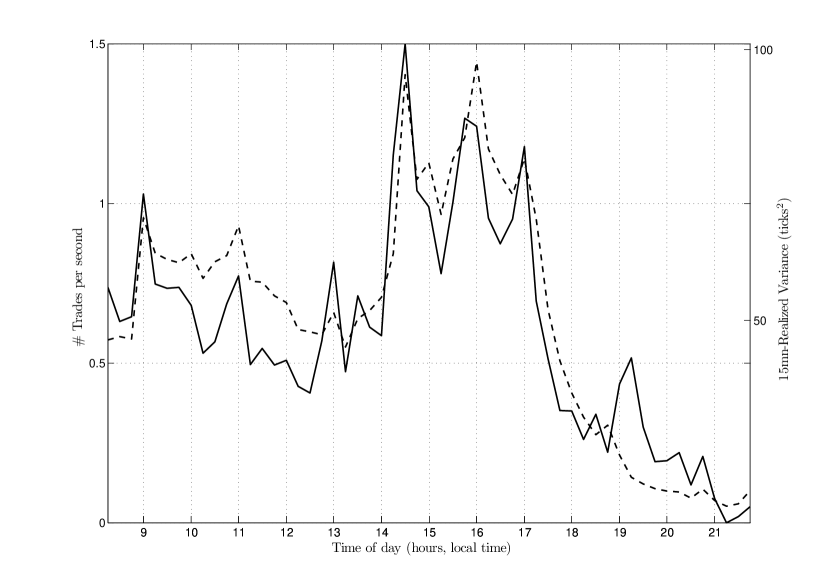
Figure 1: Bund intraday seasonality of both trading rate and volatility (abscissa are expressed in hours, local time). Averages are taken on all available days. Dashed line : average intraday rate of trading (average number of trades per second) using 15mn bins. Solid line : average 15-minutes-realized variance (estimated summing on 15 1mn-squared returns).

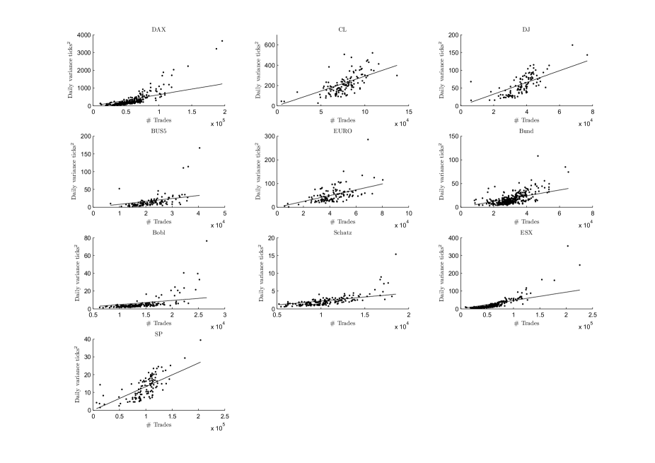
Figure 2: For each asset (in increasing perceived tick size $P_{=}$) : Daily variance (estimated summing over 5-mn quadratic returns) against daily number of trades. Each dot represents a single day. The solid line is the linear regression line with zero intercept. We see strong linearity between the variance and the number of trades but there seem to be clustering of dots above (resp. below) the solid line for days with high (resp. low) activity.

In order to have more insights, we look at some daily statistics : Fig. 2 shows a scatter plot in which each point corresponds to a given day $k$ whose abscissa is the number of trades within this day, i.e., $N_{k}$, and the ordinate is the daily variance (estimated summing over 5-mn quadratic returns) of the same day $k$. It shows that, despite some dispersion, the points are mainly distributed around a mean linear trend confirming again the idea shown in Fig. 1 that, to a good approximation, the variance is proportional to the number of trades. In that respect, trading time models (Eq. (1)) should capture most of the return variance fluctuations through the dynamics of the transaction rate. However, in Fig. 2, the points with high abscissa values (i.e., days with a lot of activity) tend to be located above the linear line, whereas the ones with low abscissa (low activity) cluster below the linear line, suggesting that the variance per trade is dependant on the daily intensity of trading.

Before moving on, we need to define a few quantities. Let $\Delta t$ be an intraday time scale and let $N$ be a number of trades. We define $V(\Delta t,N)$ as the estimated price variance over the scale $\Delta t$ conditioned by the fact that $N$ trades occurred. Using notations, 1 (vii) and (viii), from a computational point of view, when $\Delta t=\Delta t_{0}$ is fixed and $N$ is varying, $V(\Delta t=\Delta t_{0},N)$ is estimated as:

$$V(\Delta t=\Delta t_{0},N)=E_{t}\left[(p_{t+\Delta t_{0}}-p_{t})^{2}\leavevmode\nobreak\ |\leavevmode\nobreak\ NT[t,t+\Delta t_{0}]\in[N-\delta_{N},N+\delta_{N}]\right].$$ (5)

where $\delta_{N}$ is some bin size. And, along the same line, when we study $V(\Delta t,N)$ for a fixed $N=N_{0}$ value over a range of different values of $\Delta t$, one defines a temporal bin size $\delta_{\Delta t}$ and computes $V(\Delta t,N=N_{0})$ as

$$V(\Delta t,N=N_{0})=E_{i}\left[(p_{t_{i+N_{0}}}-p_{t_{i}})^{2}\leavevmode\nobreak\ |\leavevmode\nobreak\ t_{i-1+N_{0}}-t_{i-1}\in[\Delta t-\delta_{\Delta t},\Delta t+\delta_{\Delta t}]\right].$$ (6)

Let us note that, in both cases, the bins are chosen such that each bin involves approximately the same number of terms. We also define the corresponding conditional variance per trade as:

$$v(\Delta t,N)=\frac{V(\Delta t,N)}{N}.$$ (7)

In order to test the presence of an eventual non-linear behavior in the last scatter plots (Fig. 2), we show in Fig. 3 the 5-minutes variance per trade $v(\Delta t=5mn,N)$ as a function of the average intertrade duration $\frac{5mn}{N}$ as $N$ is varying. We clearly see that the estimated curve (solid line) is below the simple average variance (dashed line) for large intertrade durations and above the average variance when the trades are less than $600$ milliseconds apart. Note that we observed a similar behavior for most of the futures suggesting a universal behavior.

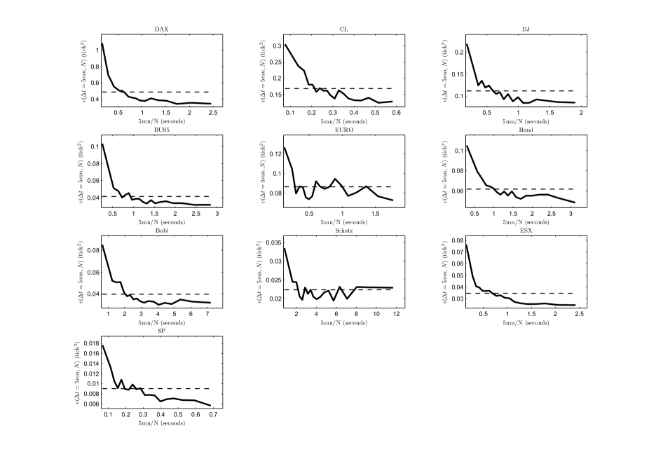
Figure 3: For each asset (in increasing perceived tick size $P_{=}$), Solid line : conditional $v(\Delta t=5mn,N)$ variance per trade (see (5) as a function of the average intertrade duration $\frac{5mn}{N}$ when varying $N$. Dashed line : unconditional 5mn-variance per trade. The solid line is almost constant for average times above 0.6 seconds, and it increases when the trading becomes faster.

To say that the realized variance is proportional to the number of trades is clearly a very good approximation as long as the trading activity is not too high as shown both on a daily scale in Fig. 2 and on a 5mn-scale in Fig. 3. However, as soon as the trading activity is high (e.g., average intertrade duration larger than $600ms$ on a 5mn-scale), the linear relationship seems to be lost. In the next section we will focus on the impact associated with a single trade.

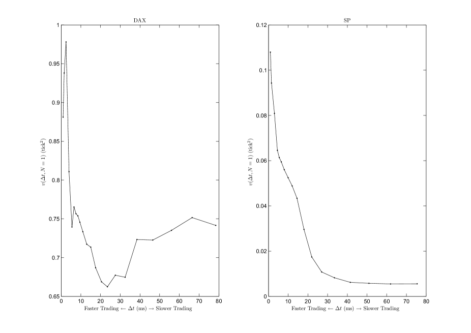
Figure 4: $v(\Delta t,N=1)$ as a function of $\Delta t$ over very short $\Delta t$’s for DAX and SP. The variance per trade increases dramatically below a certain $\Delta t$.

4 Single trade impact on the midpoint price

In this section, we will mainly focus on the impact of a trade $i$, and more specifically on the influence of its arrival time $t_{i}$ on the return $r_{t_{i}}=p_{t_{i+1}}-p_{{t_{i}}}$. In order to do so, it is natural to consider the return $r_{t_{i}}$ conditioned by $t_{i}-t_{i-1}$, the time elapsed since previous transaction. We want to be able to answer questions such as : how do compare the impacts of the $i$th trade depending on the fact that it arrived right after or long after the previous trade ? Of course, in the framework of trading time models this question has a very simple answer : the impacts are the same ! Let us first study the conditional variance of the returns.

4.1 Impact on the return variance

In order to test the last assertion, we are naturally lead to use Eqs (6) and (7) for $N_{0}=1$, i.e,

$$v(\Delta t,N=1)=E_{i}\left[r_{{t_{i}}}^{2}\leavevmode\nobreak\ |\leavevmode\nobreak\ t_{i}-t_{i-1}\in[\Delta t-\delta_{\Delta t},\Delta t+\delta_{\Delta t}]\right].$$ (8)

Let us illustrate our purpose on the DAX and the SP futures. They trade on two different exchanges, (EUREX and CME) and have very different daily statistics (e.g., DAX has the smallest perceived tick and SP the largest as one can see in Table 1). Fig. 4 shows for both assets $v(\Delta t,N=1)$ (expressed in squared $tick$) as a function of $\Delta t$ (in milliseconds). We notice that both curves present a peak for very small $\Delta t$ and stabilize around an asymptotic constant value for larger $\Delta t$. This value is close to $0.7$ ticks² for the DAX and to $0.005$ ticks² for the SP. The peak reaches $0.95$ ($35\%$ above the asymptote) for the DAX, and $0.1$ ($2000\%$ above the asymptote).

Figure 5: For each asset (in increasing perceived tick size $P_{=}$), $v(\Delta t,N=1)$ as a function of $\Delta t$ (logarithm scale). We see an "explosion" of the variance when the trading is getting faster.

Fig. 5 switches (for all assets) to a log scale in order to be able to look at a larger time range. A quick look at all the assets show that they present a very similar behavior. One sees in particular for the ESX curve that the variance increases almost linearly with the rate of trading, and then suffers an explosion as $\Delta t$ becomes smaller than 20 ms. The "same" explosion can be qualitatively observed over all assets albeit detailed behavior and in particular the minimal threshold $\Delta t$ may vary for different assets.

Let us note that the variance $v(\Delta t,N=1)$ as defined by (8) can be written in the following way:

$$v(\Delta t,N=1)=P(\Delta t)A(\Delta t),$$ (9)

where $P(\Delta t)$ is the probability for the return to be non zero conditioned by the intertrade duration $t_{i}-t_{i-1}=\Delta t$, i.e.,

$$P(\Delta t)=Prob\{r_{{t_{i}}}\neq 0\leavevmode\nobreak\ |\leavevmode\nobreak\ t_{i}-t_{i-1}\in[\Delta t-\delta_{\Delta t},\Delta t+\delta_{\Delta t}]\}$$ (10)

and where $A(\Delta t)$ is the expectation of the squared return conditioned by the fact that it is not zero and by the intertrade duration $t_{i}-t_{i-1}=\Delta t$, i.e.,

$$A(\Delta t)=E_{i}\left[r_{{t_{i}}}^{2}\leavevmode\nobreak\ |\leavevmode\nobreak\ r_{{t_{i}}}\neq 0\leavevmode\nobreak\ {\mbox{and}}\leavevmode\nobreak\ t_{i}-t_{i-1}\in[\Delta t-\delta_{\Delta t},\Delta t+\delta_{\Delta t}]\right]$$ (11)

Figure 6: For each asset (in increasing perceived tick size $P_{=}$), Probability $P(\Delta t)$ as defined by (10) as a function of $\Delta t$. We see that the probability of getting a price move increases with market order rate for most assets.

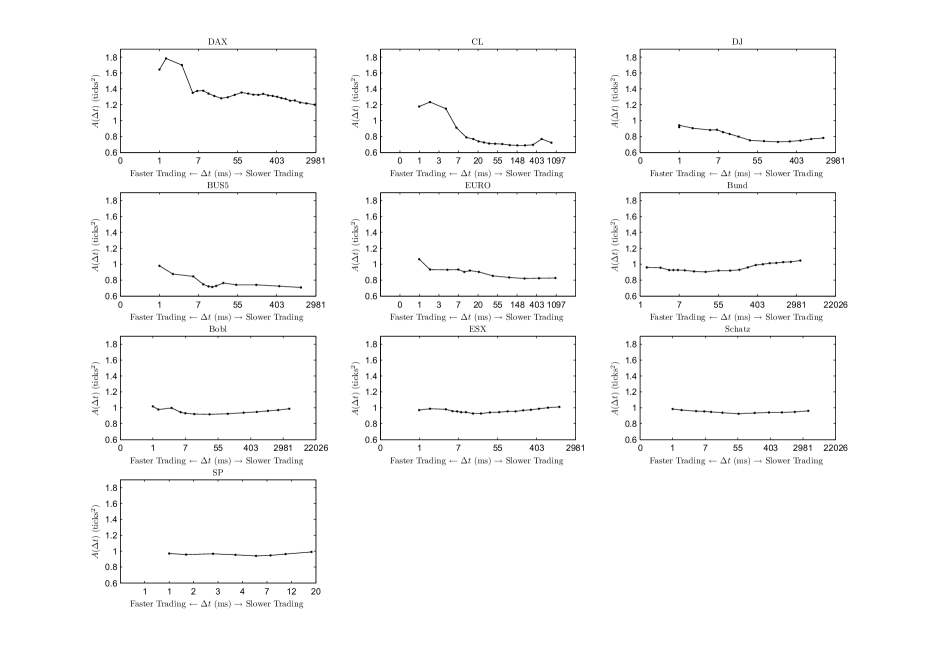
Figure 7: For each asset (in increasing perceived tick size $P_{=}$), Size of Absolute squared returns $A(\Delta t)$ as a function pf $\Delta t$. For very small tick assets, like DAX and CL we see that the absolute size of a return increases with the rate of market orders. This propriety quickly stops being true as the tick increases. The orderbook of a large tick asset is generally much thicker than that of a small tick asset and therefore it is extremely hard to to empty more than one level.

In short $P(\Delta t)$ is the probability that the midpoint price moves while $A(\Delta t)$ is the squared amplitude of the move when non-zero. In Fig. 6, we have plotted, for all assets, the function $P(\Delta t)$ for different $\Delta t$. One clearly sees that, as the trading rate becomes greater ($\Delta t\rightarrow 0$), the probability to observe a move of the midpoint price increases. One mainly recovers the behavior we observed for the analog variance plots. Let us notice that (except for the DAX), the values of the moving probabilities globally decrease as the perceived ticks $P_{=}$ increases (for large ticks, e.g. SP, at very low activity this probability is very close to zero). The corresponding estimated moving squared amplitudes $A(\Delta t)$ are displayed in Fig. 7. It appears clearly that, except for the smallest perceived ticks assets (DAX and CL basically), the amplitude can be considered as constant. This can be easily explained : large tick assets never make moves larger than one tick while small tick assets are often “perforated” by a market order. One can thus say that, except for very small ticks assets, the variance increase in high trading rate period is mostly caused by the increase of the probability that a market order absorb only the first level of the book (best bid or best ask). There is hardly no perforation of the book on the deeper levels.

4.2 Impact on the return

Before moving to the next section, let us just look at the direct impact on the return itself, as defined for instance by [3], conditioned by the intertrade time:

$$I(\Delta t,N=1)=E_{i}\left[\varepsilon_{i}r_{{t_{i}}}|t_{i}-t_{i-1}=\Delta t\right].$$ (12)

According to [15], we expect the impact to be correlated with the variance per trade and therefore for $I(\Delta t)$ to follow a very similar shape to that of $v(\Delta t,N=1)$ shown in Fig. 5 . This is confirmed in Fig. 8 where one sees that, for all assets, the impact goes from small values for large intertrade intervals to significantly higher values for small intertrade durations.

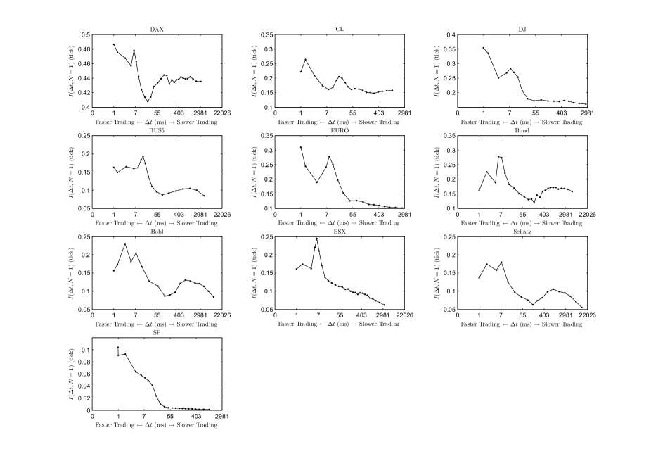
Figure 8: For each asset (in increasing perceived tick size $P_{=}$), $I(N=1|\Delta t)$ as defined by (12) as a function of $\Delta t$. The shape of the curves confirms the idea that the impact is high correlated with the variance per trade.

5 From fine to coarse

5.1 Large scale conditional variance and impact

Figure 9: For each asset (in increasing perceived tick size $P_{=}$), $v(\Delta t,N=100)$, as defined by (7), as a function of $\Delta t$. Clearly the variance of a speedy $100$ trades is higher than the variance of $100$ slow trades.

Figure 10: For each asset (in increasing perceived tick size $P_{=}$), $I(\Delta t,N=200)$, as defined by (13), as a function of $\Delta t$. The impact of speedy trades propagates well into the future. Even $200$ trades away, one speedy trade has caused more impact than a slower one.

One of the key issue associated to our single trade study is the understanding of the consequences of our findings to large scale return behavior. This question implies the study of (conditional) correlations between successive trades, which is out of the scope of this paper and will be addressed in a forthcoming work. However one can check whether the impact or the variance averaged locally over a large number of trades still display a dependence as respect to the trading rate. Indeed, in Fig. 3 we have already seen that this feature seems to persist when one studies returns over a fixed time (e.g., 5 min) period conditioned by the mean intertrade duration over this period. Along the same line, one can fix a large $N=N_{0}$ value and compute $v(\Delta t,N=N_{0})$ and $I(\Delta t,N=N_{0})$ as functions of $\Delta t$. Note that $v(\Delta t,N=N_{0})$ is defined in Eq. (7) while the aggregated impact can be defined similarly as:

$$I(\Delta t,N=N_{0})=E_{i}\left[\epsilon_{i}(p_{t_{i+N_{0}}}-p_{t_{i}})\leavevmode\nobreak\ |\leavevmode\nobreak\ t_{i-1+N_{0}}-t_{i-1}\in[\Delta t-\delta_{\Delta t},\Delta t+\delta_{\Delta t}]\right].$$ (13)

In Fig. 9 and 10 are plotted respectively the variance $v(\Delta t,N=100)$ and the return impact $I(\Delta t,N=200)$ as functions of $\Delta t$. One sees that at these coarse scales, the increasing of these two quantities as the activity increases is clear (except maybe for the variance of the EURO). As compared to single trade curves, the threshold-like behavior are smoothed out and both variance and return impacts go continuously from small to large values as the trading rate increases.

5.2 Liquidity decreases when trading rate increases

One possible interpretation of these results would be that when the trading rate gets greater and greater, the liquidity tends to decrease, i.e., the order book tends to empty.

In [15], the authors mention that the spread is an indicator of the thinness of the book and that the distance from the best bid or ask to the next level of the order book is in fact equivalent to the spread. Moreover, they bring empirical evidence and theoretical no-arbitrage arguments suggesting that the spread and the variance per trade are strongly correlated. Accordingly, we define the mean spread over $N$ trades as

$$s_{t_{i},N}=\frac{1}{N}\sum_{k=0}^{N-1}s_{t_{i+k}},$$ (14)

and the conditional spread at the fixed scale $N=N_{0}$ as

$$S(\Delta t,N=N_{0})=E_{i}\left[s_{t_{i},N}\leavevmode\nobreak\ |\leavevmode\nobreak\ t_{i+N}-t_{i}\in[\Delta t-\delta_{\Delta t},\Delta t+\delta_{\Delta t}]\right].$$ (15)

Fig. 11 displays, for each asset, $S(\Delta t,N=100)$ as a function of $\Delta t/100$ (using log scale). One observes extremely clearly an overall increase of the spread value with the rate of trading for all assets, This clearly suggests that the order book is thinner during periods of intense trading. This seems to be a universal behavior not depending at all on the perceived tick size.

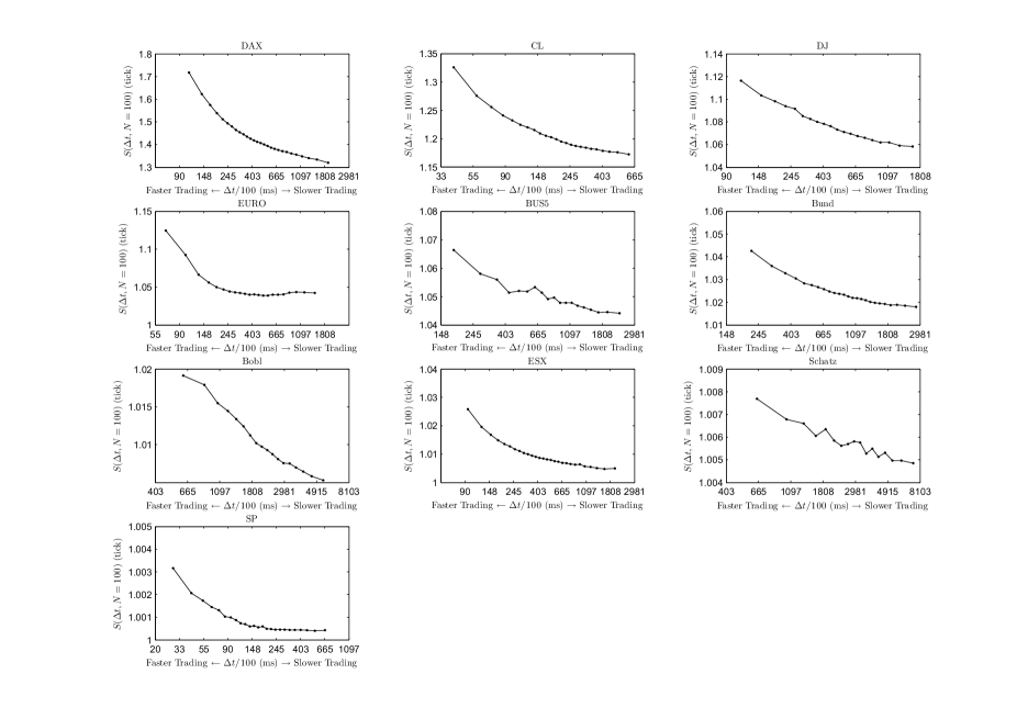
Figure 11: For each asset (in increasing perceived tick size $P_{=}$), $S(\Delta t,N=100)$ as defined in (15) as a function of $\Delta t/100$. The form of the curves confirms that there is a strong liquidity decrease when the trading rate is increasing.

6 Concluding remarks

In this short paper we provided empirical evidence gathered from high frequency futures data corresponding to various liquid futures assets that the impact (as measured from the return variance or using the standard definition) of a trading order on the midpoint price depends on intertrade duration. We have also shown that this property can also be observed at coarser scale. A similar study of the spread value confirmed the idea that order books are less filled when trading frequency is very high. Notice that we did not interpret in any causal manner our findings, i.e., we do not assert that a high transaction rates should be responsible for the fact that books are empty. It just appears that both phenomena are highly correlated and this observation has to be studied in more details. In a future work, we also plan to study the consequences of these observations on models such those described in the introductory section (Eq. (1)). A better understanding of the aggregation properties (i.e., large values of $N$) and therefore of correlations between successive trades will also be addressed in a forthcoming study.

References

- [1] Robert Almgren, Chee Thum, Emmanuel Hauptmann, and Hong Li. Direct estimation of equity market impact. Risk, July 2005.
- [2] J. P. Bouchaud and M. Potters. Theory of Financial Risk and Derivative Pricing. Cambridge University Press, Cambridge, 2003.
- [3] Jean-Philippe Bouchaud, J. D. Farmer, and Fabrizio Lillo. How markets slowly digest changes in supply and demand. In Thorsten Hens and Klaus Schenk-Hoppe, editors, Handbook of Financial Markets: Dynamics and Evolution, pages 57–156. Elsevier: Academic Press, 2008.
- [4] Jean-Philippe Bouchaud, Yuval Gefen, Marc Potters, and Matthieu Wyart. Fluctuations and response in financial markets: the subtle nature of ‘random’ price changes. Quantitative Finance, 10:176–190, April 2004.
- [5] Jean-Philippe Bouchaud, Julien Kockelkoren, and Marc Potters. Random walks, liquidity molasses and critical response in financial markets. Quantitative Finance, 6(2):115–123, 2006.
- [6] M. M. Dacorogna, R. Gençay, U. A. Müller, R. B. Olsen, and O. V. Pictet. An introduction to high frequency finance. Academic Press, 2001.
- [7] Zoltan Eisler, Bouchaud Jean-Philippe, and Julien Kockelkoren. The price impact of order book events: market orders, limit orders and cancellations. Quantitative finance papers, arXiv.org, 2010.
- [8] J. Doyne Farmer, Austin Gerig, Fabrizio Lillo, and Szabolcs Mike. Market efficiency and the long-memory of supply and demand: is price impact variable and permanent or fixed and temporary? Quantitative Finance, 6(2):107–112, April 2006.
- [9] J. Doyne Farmer, Laszlo Gillemot, Fabrizio Lillo, Szabolcs Mike, and Sen Anindya. What really causes large price changes? Quantitative Finance, 4:383–397(15), August 2004.
- [10] Jim Gatheral. No-dynamic-arbitrage and market impact. Quantitative Finance, 10(7):749–759, 2010.
- [11] László Gillemot, J. Doyne Farmer, and Fabrizio Lillo. There’s more to volatility than volume. Quantitative Finance, 6(5):371–384, 2006.
- [12] Fabrizio Lillo and J. Doyne Farmer. The long memory of the efficient market. Studies in Nonlinear Dynamics & Econometrics, 8(3), 2004.
- [13] B. B. Mandelbrot and H. W. Taylor. On the distribution of stock price differences. Operation Research, 15:1057–1062, 1967.
- [14] Christian Y. Robert and Mathieu Rosenbaum. A New Approach for the Dynamics of Ultra-High-Frequency Data: The Model with Uncertainty Zones. Forthcoming, Journal of Financial Econometrics, 2010.
- [15] Matthieu Wyart, Jean-Philippe Bouchaud, Julien Kockelkoren, Marc Potters, and Michele Vettorazzo. Relation between bid-ask spread, impact and volatility in order-driven markets. Quantitative Finance, 8(1):41–57, 2008.