Universality of rain event size distributions

Abstract

We compare rain event size distributions derived from measurements in climatically different regions, which we find to be well approximated by power laws of similar exponents over broad ranges. Differences can be seen in the large-scale cutoffs of the distributions. Event duration distributions suggest that the scale-free aspects are related to the absence of characteristic scales in the meteorological mesoscale.

1 Introduction

Atmospheric convection and precipitation have been hypothesised to be a real-world realization of self-organized criticality (SOC). This idea is supported by observations of avalanche-like rainfall events [1, 2] and by the nature of the transition to convection in the atmosphere [3, 4]. Many questions remain open, however, as summarized below. Here we ask whether the observation of scale-free avalanche size distributions is reproducible using data from different locations and whether the associated fitted exponents show any sign of universality.

Many atmospheric processes are characterized by long-range spatial and temporal correlation, and by corresponding structure on a wide range of scales. There are two complementary explanations why this is so, and both are valid in their respective regimes: structure on many scales can be the result of different processes producing many characteristic scales [5, 6]; it can also be the result of an absence of characteristic scales over some range, such that all intermediate scales are equally significant [7]. The latter perspective is relevant, for instance, in critical phenomena and in the inertial subrange of fully developed turbulence.

Processes relevant for precipitation are associated with many different characteristic time and spatial scales, see e.g. Ref. [6]. The list of these scales has a gap, however, from a few km (a few minutes) to 1,000 km (a few days), spanning the so-called mesoscale, and it is in this gap that the following arguments are most likely to be relevant.

The atmosphere is slowly driven by incident solar radiation, about half of which is absorbed by the planet’s surface, heating and moistening the atmospheric boundary layer; combined with radiative cooling at the top of the troposphere this creates an instability. This instability drives convection, which in the simplest case is dry. More frequently, however, moisture and precipitation play a key role. Water condenses in moist rising air, heating the environment and reinforcing the rising motion, and often, the result of this process is rainfall. The statistics of rainfall thus contain information about the process of convection and the decay towards stability in the troposphere. A common situation is conditional instability, where saturated air is convectively unstable, whereas dry air is stable. Under-saturated air masses then become unstable to convection if lifted by a certain amount, meaning that relatively small perturbations can trigger large responses.

Since driving processes are generally slow compared to convection, it has been argued that the system as a whole should typically be in a far-from equilibrium statistically stationary state close to the onset of instability. In the parlance of the field this idealized state, where drive and dissipation are in balance, is referred to as “Quasi-Equilibrium” (QE) [8]. In Ref. [3], using satellite data over tropical oceans, it was found that departures from the point of QE into the unstable regime can be described as triggering a phase transition whereby large parts of the troposphere enter into a convectively active phase. Assuming that the phase transition is continuous, the attractive QE state would be a case of SOC – a critical point of a continuous phase transition acting as an attractor in the phase space of a system [9, 10].

The link between SOC and precipitation processes has also been made by investigating event-size distributions in a study using data from a mid-latitude location [2]. Both the tropical data in Ref. [3] and the mid-latitude data in Ref. [2] support some notion of SOC in precipitation processes, but the climatologies in these regions are very different. Rainfall in the mid-latitudes is often generated in frontal systems, whereas in the tropics, much of the precipitation is convective, supporting high rain rates. It is not a priori clear whether these differences are relevant to the SOC analogy, or whether they are outweighed by the robust similarities between the systems. For instance, drive and dissipation time scales are well separated also in the mid-latitudes. In time series from Sweden the average duration of precipitation events was found to be three orders of magnitude smaller than the average duration of dry spells [11]. It is therefore desirable to compare identical observables from different locations.

Scale-free event size distributions suggest long-range correlation in the system, which in turn hints at a continuous transition to precipitation. Similar effects, however, can also result directly from a complex flow field, as was shown in simulations using randomized vortices and passive tracers [12]. Since the fluid dynamics is complex enough to generate apparent long-range correlation, and it is difficult from direct observation to judge whether the transition is continuous, we cannot rule out a discontinuous jump.

This uncertainty is mirrored in parameterizations of convection. The spatial resolution of general circulation models is limited by constraints in computing power to about 100 km in the horizontal. Dynamically there is nothing special about this scale, and the approach in climate modeling for representing physical processes whose relevant spatial scales are smaller is to describe their phenomenology in parameterizations. Parameterizations of convection and precipitation processes often contain both continuous and discontinuous elements. For instance, the intensity of convection and precipitation typically depends continuously on a measure of convective plume buoyancy (such as convective available potential energy) and water vapor content [8, 13], but sometimes a discontinuous threshold condition is introduced to decide whether convection occurs at all [14].

2 Data sets

We study rain data from all 10 available sites of the Atmospheric Radiation Measurement (ARM) Program, see www.arm.gov, over periods from about 8 months to 4 years, see Table 1. Precipitation rates were recorded at one-minute resolution, with an optical rain gauge, Model ORG-815-DA MiniOrg (Optical Scientific, Inc.) [15]. Data were corrected using the ARM Data Quality Reports [16], and rates below 0.2 mm/h were treated as zero measurements, as recommended by the ARM Handbook [15], see figure 1.

The measurements are from climatically different regions using a standardized technique, making them ideal for our purpose. Three sites are located in the Tropical Western Pacific (Manus, Nauru and Darwin), known for strong convective activity. Niamey is subject to strong monsoons, with a pronounced dry season. Heselbach is a mid-latitude site with an anomalously large amount of rainfall due to orographic effects. Rainfall in Shouxian is mostly convective in the summer months, which constitute most of the data set. Graciosa Island in the Azores archipelago is a sub-tropical site, chosen for the ARM program to study precipitation in low clouds of the marine boundary layer.

Three data are less straight-forward: The Point Reyes measurements specifically target Marine Stratus clouds, which dominate the measurement period and are known to produce drizzle in warm-cloud conditions (without ice phase). Unfortunately the measurements only cover six months, and it is unclear whether observed differences are due to the different physics or to the small sample size. The Southern Great Plains (SGP) measurements suffer from a malfunction that led to apparent rain rates of about 0.1 mm/h over much of the observation period. The problem seems to be present in most other data sets but is far less pronounced there, see figure 1. Measurements at temperatures below $3^{\circ}$C were discarded as these can contain snow from which it is difficult to infer equivalent rates of liquid water precipitation. The North Slope of Alaska (NSA) data set contains mostly snow; it is included only for completeness.

None of the data sets showed significant seasonal variations in the scaling exponents. In the Point Reyes, SGP and NSA data we found slight variations but could not convince ourselves that these were significant. Data from all seasons are used.

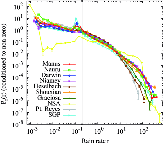
Figure 1: Probability (relative frequency) density of precipitation rate, $r$ in mm/h. The vertical line indicates the lower intensity cutoff at 0.2 mm/h. Smaller rain rates are treated as zero. The peak around 0.1 mm/h, most ponounced in the Southern Great Plains data, is due to a malfunction of the instrument. The Alaska data set contains mostly snow and is included only for completeness.

Table 1: Observation sites with corresponding time periods, number of observed precipitation events $N$, estimated annual precipitation in mm, and location.

Site	From	Until	$N$	Precip./yr	Location
Manus Island,	02/15/2005	08/27/2009	11981	5883.29	2.116∘ S, 147.425∘ E
Papua New Guinea
Nauru Island,	02/15/2005	08/27/2009	5134	1860.87	0.521∘ S, 166.916∘ E
Republic of Nauru
Darwin, Australia	02/15/2005	08/27/2009	2883	1517.09	12.425∘ S, 130.892∘ E
Niamey, Niger	12/26/2005	12/08/2006	262	608.37	13.522∘ N, 2.632∘ E
Heselbach, Germany	04/01/2007	01/01/2008	2439	2187.85	48.450∘ N, 8.397∘ E
Shouxian, China	05/09/2008	12/28/2008	480	1221.20	32.558∘ N, 116.482∘ E
Graciosa Island, Azores	04/14/2009	07/10/2010	3066	702.35	39.091∘ N, 28.029∘ E
NSA, USA	04/01/2001	10/13/2003	9097	23516.16	71.323∘ N, 156.616∘ E
Point Reyes, USA	02/01/2005	09/15/2005	579	797.85	38.091∘ N, 122.957∘ E
SGP, USA	11/06/2007	08/24/2009	1624	968.95	36.605∘ S, 97.485∘ E

3 Event sizes

The data used here are (0+1)-dimensional time series, whereas the atmosphere is a (3+1)-dimensional system. We leave the question unanswered which spatial dimensions are most relevant – the system becomes vertically unstable, but it also communicates in the two horizontal dimensions through various processes [4].

Following Ref. [2], we define an event as a sequence of non-zero measurements of the rain rate, see inset in figure 2. The event size $s$ is the rain rate, $r(t)$, integrated over the event, $s=\int_{\mathrm{event}}dt~{}r(t)$. The dimension of this object is $\left[s\right]=$mm, specifying the depth of the layer of water left on the ground during the event. One mm corresponds to an energy density of some 2500 kJ/m² released latent heat of condensation. If the rain rate were known over the area covered by the event, then the event size could be defined precisely as the energy released during one event. Since spatial information is not available, it is ignored in our study.

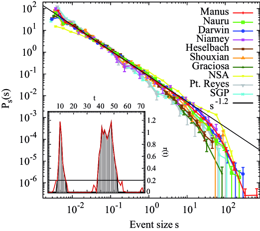
Figure 2: Probability densities of event sizes, $s$ in mm, and a power-law fit (black straight line).
Inset: Precipitation rates from Niamey, including two rain events lasting 7 and 15 minutes respectively. Interpreting reported rain rates of less than 0.2 mm/h as zero, the shaded areas are the corresponding event sizes.

For each data set, the probability density function $P_{s}(s)$ in a particular size interval $[s,s+\Delta s)$ is estimated as $P_{s}(s)\approx{n(s)}/({N\Delta s})$, where $n(s)$ is the number of events in the interval and $N$ the total number of events. We use $(s+\Delta s)/s=10^{1/5}\approx 1.58$, i.e. 5 bins per order of magnitude in $s$. Standard errors are shown, for $P_{s}(s)$: assuming Poissonian statistics, the error in $n(s)$ is approximated by $\sqrt{n(s)}$.

4 SOC scaling

Studies of simple SOC models that approach the critical point of a continuous phase transition focus on avalanche size distributions, which we liken to rain event sizes. Critical exponents are derived from finite-size scaling, that is, the scaling of observables with system size (as opposed to critical scaling, the scaling of observables with the distance from criticality). In SOC models, moments of the avalanche size distribution scale with system size $L$ like

$$\left\langle s^{k}\right\rangle\propto L^{D(1+k-\tau_{s})}\mathrm{\hskip 2.84526ptfor\hskip 2.84526pt}k>\tau_{s}-1,$$ (1)

defining the exponent $D$, sometimes called the avalanche dimension, and the exponent $\tau_{s}$, which we call the avalanche size exponent. Equation (1) is consistent with probability density functions $P_{s}(s)$ of the form

$$P_{s}(s)=s^{-\tau_{s}}\mathcal{G}_{s}(s/s_{\xi})\mathrm{\hskip 2.84526ptfor\hskip 2.84526pt}s>s_{l}$$ (2)

where $s_{\xi}=L^{D}$, and the scaling function $\mathcal{G}_{s}(s/s_{\xi})$ falls off very fast for large arguments, $s/s_{\xi}>1$, and is constant for small arguments, $s/s_{\xi}\ll 1$, down to a lower cutoff, $s=s_{l}$, where non-universal microscopic effects (e.g. discreteness of the system) become important.

Assuming that we have observations from an SOC system, and that a significant part of the observed avalanche sizes are in the region $s_{l}<s\ll s_{\xi}$, we expect to find a range of scales where the power law

$$P_{s}(s)=\mathcal{G}_{s}(0)s^{-\tau_{s}}$$ (3)

holds. Under sufficiently slow drive the exponent $\tau_{s}$ is believed to be robust in SOC models [17, 18]. We infer event-size distributions like in Ref. [2] from measurements in different locations and compare values for the apparent avalanche size exponent $\tau_{s}$. As a first step to assess the validity of (3) we produce log-log plots of $P_{s}(s)$ vs. $s$ and look for a linear regime, figure 2. Since the study of critical phenomena is a study of limits that cannot be reached in physical systems, the field is notorious for debates regarding the significance of experimental work, which is especially true for SOC. While an element of interpretation necessarily remains, we devise methods to maximize the objectivity of our analysis.

In our data sets, time series of rain rates from different locations, we interpret the upper limit $s_{\xi}$ of the scale-free range as an effective system size. We cannot control this size; nonetheless the scaling hypothesis, (2), can be tested using appropriate moment ratios [19]. For instance, $s_{\xi}\propto{\left\langle s^{2}\right\rangle}/{\left\langle s\right\rangle}$, provided $s_{l}\ll s_{\xi}$. Hence, to account for changes in effective system sizes the $s$-axis in figure 2 can be rescaled to $s{\left\langle s\right\rangle}/{\left\langle s^{2}\right\rangle}$, see figure 3. This collapses the loci of the large-scale cutoffs. Plotting $P_{s}(s)s^{\tau_{s}}$ against this rescaled variable produces figure 3 of the scaling function $\mathcal{G}_{s}(s/(as_{\xi}))$, where $a$ is the proportionality constant relating $s_{\xi}$ to the moment ratio. This has the advantage of reducing the logarithmic vertical range, which makes it possible to see differences in the distributions that would otherwise be concealed visually. Figure 3 covers 9 orders of magnitude vertically, whereas figure 3 covers little more than 2.

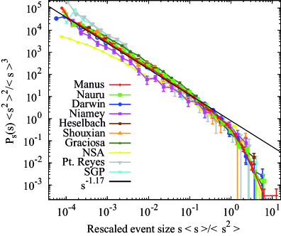
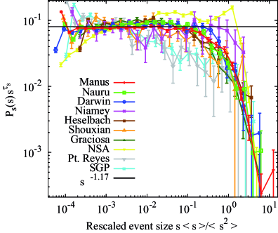
Figure 3: (a) Event size distributions rescaled with the moment ratio $\frac{\left\langle s^{2}\right\rangle}{\left\langle s\right\rangle}$. (b) Inferred scaling function $\mathcal{G}_{s}$, using $\tau_{s}=1.17$ for all data sets. By far the largest deviations from a common scaling function are observed for the unreliable data sets, Alaska (NSA) and Southern Great Plains (SGP).

5 Exponent estimation and goodness of fit

For a detailed discussion, see A. We apply a form of Kolmogorov-Smirnov (KS) test [20] similar to that in Ref. [21]. First, a fitting range $[s_{\mathrm{min}},s_{\mathrm{max}}]$ is selected. In this range the maximum-likelihood value for $\tau_{s}$ in (3) is found. Next, the maximum difference between the empirical cumulative distribution in this range and the cumulative distribution corresponding to the best-fit power law is found. The same measure is applied to synthetic samples of data (each with the same number of instances), generated from the best-fit power-law distribution. This yields the “p”-value, i.e. the fraction of samples generated from the tested model (the best-fit power law) where at least such a difference is observed. We stress that each synthetic data set is compared to its own maximum-likelihood power-law distribution, i.e. an exponent has to be fitted for each sample, so that no bias be introduced.

We keep a record of the triplet $(s_{\mathrm{min}},s_{\mathrm{max}},\tau_{s})$ if the $p-$value is greater than 10% (our arbitrarily chosen threshold). After trying all possible fitting ranges with $s_{\mathrm{min}}$ and $s_{\mathrm{max}}$ increasing by factors of $10^{0.01}$, we select the triplet which maximizes the number $\bar{N}$ of data between $s_{\mathrm{min}}$ and $s_{\mathrm{max}}$.

The distributions in figure 2 are visually compatible with a power law (black straight line) over most of their ranges. The procedure consisting of maximum-likelihood estimation plus a goodness-of-fit test confirms this result: over ranges between 2 and 4 orders of magnitude, all data sets are consistent with a power-law distribution and the estimates of the apparent exponents are in agreement with the hypothesis of a single exponent $\tau_{s}=1.17(3)$, brackets indicating the uncertainty in the last digit, except for the three problematic data sets from Point Reyes, the Southern Great Plains and Alaska. The complete results are collected in Table 2. While the best-fit exponents in this table are surprisingly similar (given the climatic differences between the measuring sites), the error estimates are unrealistically small. Taking the statistical results literally, we would have to conclude that the exponents are very similar but mutually incompatible (e.g. $\tau_{s}{{}^{\mathrm{Manus}}}=1.18(1)$ and $\tau_{s}{{}^{\mathrm{Nauru}}}=1.14(1)$) suggesting that $\tau_{s}$ is not universal. On physical grounds we do not believe this conclusion because systematic errors arising from the measurement process, the introduction of the sensitivity threshold, binning during data recording etc., are likely to be much larger than the purely statistical errors quoted here. For example, Ref. [2] used a different type of measurement with a smaller sensitivity threshold and led to a best estimate for the exponent of 1.36. Furthermore, the apparent exponent can only be seen as a rough estimate of any true underlying exponent. We tested that, fixing $\tau_{s}=1.17$, all data sets yield $p>10\%$ over a range larger than two and a half orders of magnitude, except for the three problematic data sets. A two-sample Kolmogorov-Smirnov test for all pairs of datasets further confirms the similarity of the distributions for the different sites, B.

In  figure 4 we show a color plot of all triplets $(s_{\mathrm{min}},s_{\mathrm{max}},\tau_{s})$, corresponding to the Manus dataset. There is a large plateau where $\tau_{s}\approx 1.17$, indicating that this value is the best estimate for many intervals. Figure 4 is an analogous plot for the $p-$value, showing that the goodness of the fit is best in the region of the plateau.

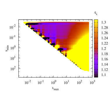
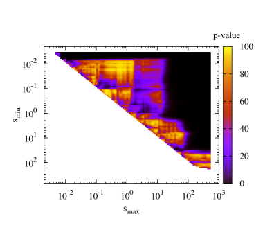
Figure 4: (a) Color map showing the best-fit value for the exponent $\tau_{s}$ for all pairs of $s_{\mathrm{min}}$ and $s_{\mathrm{max}}$, (lower and upper ends of the chosen fitting range in mm) for the Manus dataset. The large plateau corresponds to $\tau_{s}\approx 1.17$. (b) Analogous plot for the $p-$value.

Table 2: Avalanche size exponent $\tau_{s}$ for all sites (last column). Lower and upper end of fitting range (in mm), logarithmic range $s_{\mathrm{max}}/s_{\mathrm{min}}$, number of events $N$, number of events in fitting range $\bar{N}$, and a moment ratio proportional to the cutoff $s_{\xi}$ are shown. Brackets () denote errors in the last digit, determined by jackknife [22].

• Site	$s_{\mathrm{min}}$	$s_{\mathrm{max}}$	${s_{\mathrm{max}}}/{s_{\mathrm{min}}}$	$N$	$\overline{N}$	$\left\langle s^{2}\right\rangle/\left\langle s\right\rangle(er)$	$\tau_{s}(er)$
  Manus	0.0069	18.7	2719.	11981	9320	53.(1)	1.19(1)
  Nauru	0.0066	4.7	704.	5134	3996	37.(1)	1.14(1)
  Darwin	0.0067	21.6	3230.	2883	2410	50.(1)	1.16(1)
  Niamey	0.0041	55.0	13500.	262	232	25.(2)	1.19(3)
  Heselbach	0.0072	1.4	195.	2439	1764	13.(1)	1.18(2)
  Shouxian	0.0037	2.5	677.	480	406	39.(2)	1.19(3)
  Graciosa	0.0069	1.0	148.	3066	2260	14.4(3)	1.16(1)
  NSA	0.0205	5.9	288.	9097	6030	47.(1)	1.01(1)
  Pt. Reyes	0.0062	66.7	10796.	579	427	37.(2)	1.40(2)
  SGP	0.0062	58.8	9463.	1624	1196	27.(1)	1.40(2)

Climatic differences between regions are scarcely detectable in event size distributions, which may be surprising on the grounds of climatological considerations. However, the cutoff $s_{\xi}$, representing the capacity of the climatic region around a measuring site to generate rain events, changes significantly from region to region, confirming meteorological intuition. This is difficult to see in the logarithmic scales of figure 2 but is easily extracted from the moments of the distributions, Table 2. Thus, the smallest cutoff (and likely maximum event size) in the ARM data is found in Heselbach (mid-latitudes), whereas the largest is in Manus (Western Pacific warm pool). We note that $\left\langle s^{2}\right\rangle/\left\langle s\right\rangle$ is only proportional to the actual cutoff $s_{\xi}$. Assuming a box function for the scaling function and using the value $\tau_{s}=1.17$, we can estimate the proportionality constant and find $s_{\xi}\approx 2.2\left\langle s^{2}\right\rangle/\left\langle s\right\rangle$. With this estimate, none of the fitting ranges extends beyond the cutoff.

6 Dry spells

The durations of precipitation-free intervals have also been reported to follow an approximate power law [2]. We therefore repeat for dry-spell durations the same analysis as for the event sizes. Figure 5 shows the distributions, with a collapse corresponding to figure 3 in figure 5. We notice the different strengths of the diurnal cycle, here visible as a relative peak near 1 day dry spell duration. Exponents fitted to the distributions are similar, see table 3.

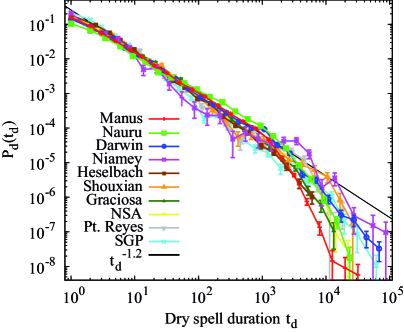
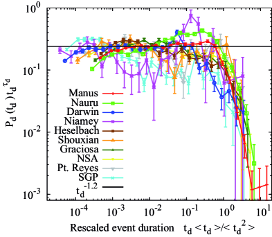
Figure 5: (a) Probability densities for dry spell durations (in min). The diurnal cycle is most pronounced in Niamey, otherwise the distributions are similar. (b) Distributions collapsed onto their scaling function, similar to figure 3.

Table 3: Dry spell exponent (last column). Lower and upper end of fitting range (in min), logarithmic range ${t_{d}}_{\mathrm{max}}/{t_{d}}_{\mathrm{min}}$, number of dry spells in data set, $N$, and number of dry spells in the fitting range $\bar{N}$, and a moment ratio proportional to the cutoff are shown are shown. Brackets () denote errors in the last digit, determined by jackknife. The number of dry spells need not be within $\pm 1$ of the number of events, as our definition of an event (and a dry spell) implies that it can be split in two if it contains an erroneous measurement. Note the magnitude of this effect in the NSA data set.

• Site	${t_{d}}_{\mathrm{min}}$	${t_{d}}_{\mathrm{max}}$	${t_{d}}_{\mathrm{max}}/{t_{d}}_{\mathrm{min}}$	$N$	$\overline{N}$	$\left\langle{t_{d}}^{2}\right\rangle/\left\langle t_{d}\right\rangle(er)$	$\tau_{d}(er)$
  Manus	24.4	1363.1	55.8	11992	4505	2149.(20)	1.16(2)
  Nauru	7.5	1027.5	137.7	5126	2912	3557.(50)	0.99(2)
  Darwin	8.5	3660.6	432.6	2892	1595	19477.(368)	1.17(1)
  Niamey	2.4	1774.0	726.1	262	135	26386.(1699)	1.33(5)
  Heselbach	9.5	5748.0	605.4	2441	1035	2043.(34)	1.37(2)
  Shouxian	2.7	13488.5	4957.1	478	365	8776.(404)	1.27(3)
  Graciosa	14.6	415.2	28.5	3068	1185	2943.(49)	1.28(3)
  NSA	12.2	9033.2	739.7	3440	1531	4293.(73)	1.3(2)
  Pt. Reyes	3.6	17141.0	4826.3	579	379	5513.(233)	1.27(2)
  SGP	8.4	2248.7	268.5	1625	523	17243.(463)	1.46(3)

7 Event durations

Precipitation event duration distributions are broad for all locations. Durations provide a link to studies of geometric properties of precipitation fields. Numerous studies of tropical deep convective rain fields [23], shallow convection fields [24], clouds [25, 26, 27, 28], and model data from large eddy simulations [29] have reported the distributions of ground covered by events (in radar snap shots etc.) to be well approximated by power laws. We note that in the clustering null model of critical two-dimensional percolation, clusters defined in one-dimensional cuts, akin to durations, do not scale, whereas two-dimensional clusters, akin to cloud-projections, do.

Applying to the durations the methods we used for the event sizes, we find comparatively short power-law ranges, see table 4. The scaling range, if it exists, is expected to be smaller than for event sizes as the size distribution is a complicated convolution of the event duration and precipitation rate distributions, figure 1, whose product covers a broader range than either of the distributions alone. The event size distribution is broader than the duration distribution also because long events tend to be more intense (not shown).

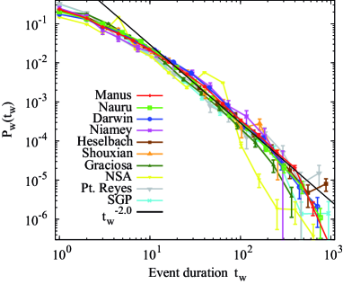
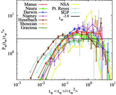
Figure 6: (a) Probability densities for event durations (in min) are broad for all data sets. From a few min up to a few hundred min a power law with an exponent $\tau_{m}\approx 2.0$ roughly describes the data. (b) Collapsed distributions, similar to figure 3.

Table 4: Duration exponent (last column). Lower and upper end of fitting range (in min), logarithmic range ${t_{w}}_{\mathrm{max}}/{t_{w}}_{\mathrm{min}}$, number of events in data set, $N$, and number of events in the fitting range $\bar{N}$ are shown. Brackets () denote errors in the last digit, determined by jackknife.

• Site	${t_{w}}_{\mathrm{min}}$	${t_{w}}_{\mathrm{max}}$	${t_{w}}_{\mathrm{max}}/{t_{w}}_{\mathrm{min}}$	$N$	$\overline{N}$	$\left\langle{t_{w}}^{2}\right\rangle/\left\langle t_{w}\right\rangle$	$\tau_{w}(er)$
  Manus	34.4	641.9	18.7	11981	1200	122.(1)	2.12(4)
  Nauru	25.4	437.5	17.2	5134	540	106.(1)	2.09(6)
  Darwin	17.87	89.30	5.00	2883	554	109.(2)	2.0(1)
  Niamey	2.7	211.8	78.4	262	157	79.(5)	1.39(7)
  Heselbach	18.2	1005.0	55.1	2439	388	261.(5)	1.97(6)
  Shouxian	7.7	197.5	25.5	480	172	84.(4)	1.73(9)
  Graciosa	12.7	424.0	33.4	3066	512	60.(1)	2.12(6)
  NSA	75.2	103.3	1.4	9097	16	49.(1)	6.(3)
  Pt. Reyes	5.7	784.0	138.6	579	178	272.(1)	1.71(7)
  SGP	9.4	278.2	29.7	1624	303	143.(4)	1.74(7)

8 Conclusions

We find that the apparent avalanche size exponents, measured with identical instruments in different locations, are consistent with a single value of $\tau_{s}=1.17(3)$ for all reliable data sets. We note that the data sets from Point Reyes and from the Southern Great Plains are similar in many respects, despite the different reasons for treating them with suspicion.

The statistical error in this estimate is surprisingly small, but neither the value itself nor the error change much using different fitting techniques or introducing different sensitivity thresholds (not shown). Nonetheless we believe systematic errors to be larger. Thus, the analysis gives an impression of the universality of the result but not necessarily the physical “true” value of the exponent. This does not contradict the climatological situation – tropical regions, for instance, are expected to support larger events than mid-latitude locations, which could be realized as a smaller exponent value $\tau_{s}$. While the exponents are not significantly different, the larger tropical events are reflected in the greater large-scale cutoff of the tropical distributions. Similarly, the dry-spell durations seem to follow another power law with $\tau_{d}=1.2(1)$, and regional differences can be seen in the strength of the diurnal cycle and the cutoff dry spell duration. The broad range of event durations, figure 6, suggests a link to the lack of characteristic scales in the mesoscale regime, where approximately scale-free distributions of clusters of convective activity, for example cloud or precipitation, have been observed to span areas between $\mathcal{O}$(1 km²) and $\mathcal{O}$(10⁶ km²) [24, 23, 29, 27, 25]. The observation of scale-free rainfall event sizes suggests long-range correlation in the pertinent fields, a possible indication of critical behaviour near the transition to convective activity. Direct measurements of the behaviour of the correlation function for the precipitation field under changes of the (much more slowly varying) background fields of water vapor and temperature are desirable to clarify whether the long range correlation is a consequence of the flow field, of the proximity to a critical point, or of a combination of both.

Appendix A Fitting procedure

In order to obtain reliable values of, for example, the exponent $\tau_{s}$, independent of the binning procedure used for the plots of $P_{s}(s)$, we use maximum likelihood estimation. We assume a power-law distribution $P_{s}(s)=a_{\tau_{s}}s^{-\tau_{s}}$, with support $[s_{\mathrm{min}},s_{\mathrm{max}}]$. Normalization yields $a_{\tau_{s}}=(1-\tau_{s})/(s_{\mathrm{max}}^{1-\tau_{s}}-s_{\mathrm{min}}^{1-\tau_{s}}$) for a given value of $\tau_{s}$.

We compute the log-likelihood function,

$$\mathcal{L}:=\ln\prod_{i=1}^{\bar{N}}P_{s}(s_{i})=\sum_{i=1}^{\bar{N}}\ln\left(a_{\tau_{s}}{s_{i}}^{-\tau_{s}}\right)$$ (4)

where the index $i$ runs over all $\bar{N}$ events whose size $s_{i}$ is between $s_{\mathrm{min}}$ and $s_{\mathrm{max}}$. Holding $s_{\mathrm{min}}$ and $s_{\mathrm{max}}$ fixed, the value of $\tau_{s}$ which maximizes $\mathcal{L}$ is the maximum likelihood estimate of the exponent. Uncertainties in $\tau_{s}$ are determined using the jackknife method.

The goodness of the fit is assessed by a Kolmogorov-Smirnov (KS) test [20]. The KS statistic, or KS distance, $d$, is defined as

$$d:=\displaystyle\max_{s_{\mathrm{min}}\leq s\leq s_{\mathrm{max}}}|S_{\bar{N}}(s)-F_{s}(s)|$$ (5)

where $S_{\bar{N}}(s)$ denotes the empirical cumulative distribution, defined as the fraction of observed events with a size smaller than $s$, in the interval $[s_{\mathrm{min}},s_{\mathrm{max}}]$. Thus, ordering the observed values by size, $s_{1}\leq\dots\leq s_{i}\leq s_{i+1}\dots\leq s_{\bar{N}}$, we have $S_{\bar{N}}(s)=i/\bar{N}$ if $s_{i}<s\leq s_{i+1}$; $F_{s}$ denotes the cumulative distribution of the maximum-likelihood distribution, $F_{s}(s):=\int_{s_{\mathrm{min}}}^{s}P_{s}(t)dt$.

The KS distance translates into the $p-$value. The $p-$value is the probability that synthetic data, here drawn from a power law distribution with exponent $\tau_{s}$, result in a KS-distance of at least $d$. For instance, $p=10\%$ means that for power-law distributed data with exponent $\tau_{s}$ there is a probability of 0.90 that the KS distance takes a value smaller than $d$. Thus, if the data really are generated by a power law and we decide to reject the power law as a model if $p<10\%$, we will reject the correct model in 10% of our tests. Conversely, decreasing the limit of rejection in the $p-$value implies that we accept more false models.

In our implementation of the KS test the distribution to be tested, $P_{s}(s)$, is not independent of the empirical data. This is because the exponent $\tau_{s}$ is obtained from the data that are later used to test the distribution. We therefore cannot use the standard analytic expression for $p(d)$, see Ref. [20], Ch. 15. Instead, we determine the distribution of the KS distance and therefore the $p-$value by means of Monte Carlo simulations: we generate synthetic power-law-distributed data sets between $s_{\mathrm{min}}$ and $s_{\mathrm{max}}$ with exponent $\tau_{s}$ and number of data $\bar{N}$ (see Table 2), and proceed exactly in the same way as for the empirical data, first obtaining a maximum likelihood estimate of the exponent $\tau_{s}$ and then computing the KS distance between the empirical distribution of the simulated data and the fitted distribution containing the estimated value of $\tau_{s}$. The $p-$value is obtained as the fraction of synthetic data sets for which the KS statistic is larger than the value obtained for the empirical data.

The final step is to compare results for different ranges $[s_{\mathrm{min}},s_{\mathrm{max}}]$. We try all possible fitting ranges with $s_{\mathrm{min}}$ and $s_{\mathrm{max}}$ increasing by factors of $10^{0.01}\approx 1.023$. We choose to report those intervals $[s_{\mathrm{min}},s_{\mathrm{max}}]$ that contain the largest number of events $\bar{N}$ with a corresponding $p-$value larger than 10%.

Appendix B Two-sample Kolmogorov-Smirnov Tests

A two-sample Kolmogorov-Smirnov test was performed for each pair of data sets, $i,j$ to test whether the two underlying event-size probability distributions differ. This test does not assume any functional form for the probability distributions [20]. As in the fitting of the exponent, we vary the testing ranges $[s_{\mathrm{min}},s_{\mathrm{max}}]$, keeping those which yield $p>10\%$. We report the range with the maximum effective number of data, $\bar{N}_{\mathrm{eff}}\equiv\bar{N_{i}}\bar{N_{j}}/(\bar{N_{i}}+\bar{N_{j}})$. The results, shown in Table 5, confirm that the pairs of distributions from the reliable data sets are similar over broad ranges.

Table 5: Maximum range $s_{\mathrm{max}}/s_{\mathrm{min}}$ over which the $p$-value of of a two-sample KS test is greater than 10%.

	Nauru	Darwin	Niamey	Heselbach	Shouxian	Graciosa	NSA	Pt. Reyes	SGP
Manus	5386.	16257.	16386.	679.	6355.	638.	14.	32.	8.
Nauru	-	6753.	13495.	236.	221.	342.	27.	19.	7.
Darwin	-	-	12247.	236.	271.	575.	27.	16.	5.
Niamey	-	-	-	3466.	16420.	2358.	1599.	668.	253.
Heselbach	-	-	-	-	14600.	13265.	18.	20.	5.
Shouxian	-	-	-	-	-	26440.	13.	65.	39.
Graciosa	-	-	-	-	-	-	11.	17.	589.
NSA	-	-	-	-	-	-	-	10.	3.
Pt. Reyes	-	-	-	-	-	-	-	-	19916.

References

References

- [1] Andrade R F S, Schellnhuber H J, and Claussen M. Analysis of rainfall records: possible relation to self-organized criticality. Physica A, 254(3-4):557–568, 1998.
- [2] Peters O, Hertlein C, and Christensen K. A complexity view of rainfall. Phys. Rev. Lett., 88(1):018701(1–4), 2002.
- [3] Peters O and Neelin J D. Critical phenomena in atmospheric precipitation. Nature Phys., 2(6):393–396, 2006.
- [4] Neelin J D, Peters O, and Hales K. The transition to strong convection. J. Atmos. Sci., 66(8):2367–2384, 2009.
- [5] Klein R. Scale-dependent models for atmospheric flows. Anu. Rev. Fluid Mech., 42:249–274, 2010.
- [6] Bodenschatz E, Malinowski S P, Shaw R A, and Stratmann F. Can we understand clouds without turbulence? Science, 327(5968):970–971, 2010.
- [7] Barenblatt G I. Scaling, Self-similarity and Intermediate Asymtotics. Cambridge University Press, Cambridge, 1996.
- [8] Arakawa A and Schubert W H. Interaction of a cumulus cloud ensemble with large-scale environment. J. Atmos. Sci., 31(3):674–701, 1974.
- [9] Tang C and Bak P. Critical exponents and scaling relations for self-organized critical phenomena. Phys. Rev. Lett., 60(23):2347–2350, 1988.
- [10] Dickman R, Vespignani A, and Zapperi S. Self-organized criticality as an absorbing-state phase transition. Phys. Rev. E, 57(5):5095–5105, 1998.
- [11] Olsson J, Niemczynowicz J, and Berndtsson R. Fractal analysis of high-resolution rainfall time-series. J. Geophys. Res., 98(D12):23265–23274, 1993.
- [12] Dickman R. Rain, power laws, and advection. Phys. Rev. Lett., 90(10):108701(1–4), 2003.
- [13] Betts A K and Miller M J. A new convective adjustment scheme. Part II: Single column tests using gate wave, bomex, atex and arctic air-mass data sets. Q. J. R. Meteorol. Soc., 112(473):693–709, 1986.
- [14] J D Neelin, O Peters, J W B Lin, K Hales, and C E Holloway. Rethinking convective quasi-equilibrium: observational constraints for stochastic convective schemes in climate models. Phil. Trans. R. Soc. A, 366:2581–2604, 2008.
- [15] Ritsche M T. ARM surface meteorology systems handbook and surface meteorology (smet) handbook. http://www.arm.gov/publications/handbooks.
- [16] ARM data quality program. http://www.arm.gov/data/data_quality.stm.
- [17] Alava M J, Laurson L, Vespignani A, and Zapperi S. “Comment on Self-organized criticality and absorbing states: Lessons from the Ising model”. Phys. Rev. E, 77(4):048101(1–2), 2008.
- [18] Pruessner G and Peters O. Reply to “Comment on “Self-organized criticality and absorbing states: Lessons from the Ising model””. Phys. Rev. E, 77(4):048102(1–2), 2008.
- [19] Rosso A, Le Doussal P, and Wiese K J. Avalanche-size distribution at the depinning transition: A numerical test of the theory. Phys. Rev. B, 80(14):144204(1–10), 2009.
- [20] Press W H, Teukolsky S A, Vetterling W T, and Flannery B P. Numerical Recipes. Cambridge University Press, Cambridge, 3rd edition, 2002.
- [21] Clauset A, Shalizi C R, and Newman M E J. Power-law distributions in empirical data. SIAM Rev., 51(4):661–703, 2009.
- [22] Efron B. The jackknife, the bootstrap and other resampling plans. CBMS-NSF Regional Conference Series in Applied Mathematics, Monograph 38, SIAM, Philadelphia., 1982.
- [23] Peters O, Neelin J D, and Nesbitt S W. Mesoscale convective systems and critical clusters. J. Atmos. Sci., 66(9):2913–2924, 2009.
- [24] Trivej P and Stevens B. The echo size distribution of precipitating shallow cumuli. J. Atmos. Sci., 67(3):788–804, 2010.
- [25] Cahalan R F and Joseph J H. Fractal statistics of cloud fields. Mon. Wea. Rev., 117(2):261–272, 1989.
- [26] B E Mapes and R A Houze Jr. Cloud clusters and superclusters over the Oceanic Warm Pool. Mon. Wea. Rev., 121:1398–1415, 1993.
- [27] Benner T C and Curry J A. Characteristics of small tropical cumulus clouds and their impact on the environment. J. Geophys. Res., 103(D22):28753–28767, 1998.
- [28] D. Schertzer and S. Lovejoy. The dimension and intermittency of atmospheric dynamics. In B. Launder, editor, Turbulent Shear Flows 4, pages 7–33. Springer, New York, 1985.
- [29] Neggers R A J, Jonker H J J, and Siebesma A P. Size statistics of cumulus cloud populations in large-eddy simulations. J. Atmos. Sci., 60(8):1060–1074, 2003.