Aharonov-Casher oscillations of spin current through a multichannel mesoscopic ring

Abstract

The Aharonov-Casher (AC) oscillations of spin current through a 2D ballistic ring in the presence of Rashba spin-orbit interaction and external magnetic field has been calculated using the semiclassical path integral method. For classically chaotic trajectories the Fokker-Planck equation determining dynamics of the particle spin polarization has been derived. On the basis of this equation an analytic expression for the spin conductance has been obtained taking into account a finite width of the ring arms carrying large number of conducting channels. It was shown that the finite width results in a broadening and damping of spin current AC oscillations. We found that an external magnetic field leads to appearance of new nondiagonal components of the spin conductance, allowing thus by applying a rather weak magnetic field to change a direction of the transmitted spin current polarization.

I Introduction

The Aharonov-Casher effect is a spectacular demonstration of the fundamental role of the spin-orbit interaction (SOI) in electronic transport. This effect is a non-Abelian analog of the Aharonov-Bohm effect. An electronic wave entering a two dimensional ring is splitted into two waves traveling trough the upper and the lower arms and interfering on the exit from the ring. Due to SOI the spinor components in each of the waves obtain the relative phase shift. This shift, in its turn, gives rise to a destructive or constructive interference pattern in the transmittance probability, that results in a number of oscillation effects on electron transport parameters. Notably, that in semiconductor heterostructures SOI can be varied through the gate voltage manipulation, suggesting interesting opportunities for practical applications of this effect in spintronics.

A simplest model to study the AC effect is a one-dimensional (1D) or one-channel ring with none or few scatterers of electrons. Aronov and Lyanda-Geller Aronov_LG studied oscillations of the magnetoconductance in a 1D ring in the presence of Rashba Bychkov SOI. Ya-Sha Yi et. al. Ya_Sha considered a joint effect of the Zeeman coupling, magnetic flux and SOI on the conductance of a 1D ring beyond the adiabatic approximation employed in Ref. Aronov_LG, . Nitta et. al. Nitta_theory noted that SOI alone, without the magnetic field, can cause oscillations of the ring electric conductance. Meijer et al.Meijer_1D_Hamiltonian pointed out that the Hamiltonian used earlier in Ref. Aronov_LG, was not quite correct and, in particular, was not Hermitian. Using the correct Hamiltonian Frustaglia and RichterFrustaglia revised the expression for the conductance found in Ref. Nitta_theory, .

In disordered mesoscopic systems the AC effect is strongly modified. Multiple impurity scatterings lead to averaging out of some strong oscillations that were presented in ideal 1D rings. There is a similarity to AB effect where the fundamental $h/e$ peak in the Fourier spectrum of magnetoconductance vanishes and is substituted for $h/2e$ Al’tshuler, Aronov, and Spivak AAS oscillations. Mathur and Stone Mathur have demonstrated that a similar weak localization effect takes place in the case of AC oscillations in a thin diffusive ring with Rashba SOI. They have shown that the average conductance periodically varies as a function of the SOI coupling constant with a period that is 1/2 of the ideal ring conductance oscillations. This prediction have been confirmed experimentally by Koga et al.Koga_et_al who observed that the amplitude of $h/2e$ magnetoconductance oscillations (AAS type oscillations) oscillates itself with varying the applied gate voltage and, correspondingly, the SOI strength. On the other hand, the fundamental AB, as well as AC oscillations show up in mesoscopic conductance fluctuations. The conductance correlator has been calculated in Ref. Malsh_Diffus, for a diffusive ring in the presence of Zeeman coupling and Rashba SOI. It was found that the amplitude of $h/e$ AB peak shows oscillations with varying SOI, similar to those that have been observed for the $h/2e$ peak in Ref. Koga_et_al, .

Although 1D, as well as diffusive models are useful to elucidate fundamental physical effects associated with SOI, they can not be fully applied to realistic semiconductor systems used in experiments. For example, an attempt to interpret the observed Morpurgo splitting of the AB power spectrum within the diffusion model Malsh_Diffus ; Engel_Loss was not successful. In Ref. Morpurgo, , as well as in other experimental works Koga_et_al ; Yau_Shayegan , the mesoscopic loops carry many channels. At the same time their sizes are comparable to the electron mean free path. Therefore, neither of the above theoretical models can be applied. In this situation an approach based on path integrals along classic trajectories can be fruitful. Such a method has been applied to transport in mesoscopic systems in a number of works Gutz ; JBS_chaos ; Berry_Robnik ; JBS_Blum_Smil . It was also employed for calculation of the spin conductance through a classically chaotic and regular cavities and rings with Rashba SOI Malsh ; Cheng_Hung . In Ref.Malsh, it was done analytically by applying the method of trajectory averaging, while numerical simulations of path integrals were performed in Ref.Cheng_Hung, . In both cases pronounced AC oscillations of the spin conductance with varying SOI constant had been found. Their important distinction from oscillations of the electric conductance is that they appear in the main semiclassical approximation, not involving weak localization or other quantum corrections.

While in a multichannel loop studied in Ref. Malsh, the electron motion was two-dimensional, the AC phase accumulation had an effectively one-dimensional character. The reason is that in a thin enough loop SOI causes only a small variation of spinor amplitudes during particle motion along any straight segment of a trajectory. In the leading approximation ignoring AC phase fluctuations associated with a finiteness of a loop width, a phase evolution depends only on a coordinate along the loop and finite width effects vanish. On the other hand, as follows from the Monte Carlo analysis Cheng_Hung , when a particle lifetime within the ring is long enough, the finite width effect on the amplitude and shape of AC oscillations is strong.

In order to elucidate this problem we will calculate the spin conductance taking into account the finite width effect in a classically chaotic multi-channel ring with the Rashba spin-orbit interaction and a uniform magnetic field applied perpendicular to the ring. A chaotic motion of particles can be provided by non ideal boundaries of the ring, as well as by random potential variations inside it. Starting from an analog of the Landauer formula derived for the spin conductance in Appendix A, we apply the path integral method to this conductance. Within this approximation spin dependent transmission amplitudes for each of the classical paths decompose into a product of a spin independent transmission amplitude and a matrix determining evolution of spinor components along this trajectory. The expression for the spin conductance that is quadratic in these amplitudes should be double summed over the trajectories afterwards. Ignoring weak localization and other quantum corrections, only the terms diagonal with respect to the trajectories are then retained. As a result, the spin conductance takes a form of a $3\times 3$ matrix averaged over the trajectories. Based on known statistical properties of chaotic trajectories we will derive Fokker-Planck equations describing spin evolution of a particle moving through the ring and analytically calculate the average of spin conductance matrix components. The finite width effects will be analyzed that show up in an additional broadening and decreasing of AC oscillations. The magnetic field, in its turn, results in appearance of spin conductance components that were equal to zero in the absence of the field, suggesting thus an opportunity to rotate the spin polarization on the exit from the ring.

The outline of the paper is as follows. Section II contains a description of the model system we used in our theory. In section III an expression for the spin conductance is obtained in the form of a sum over classical trajectories. In section IV the Fokker-Planck equation for the spin polarization distribution function is derived. On the basis of this equation the spin conductance averaged over chaotic trajectories is calculated. The discussion of results is presented in Section V.

II The model

We consider spin transport through a 2D ring which is connected via two symmetrically placed leads to two reservoirs of electrons (see Fig. 1) and is subject to the magnetic field perpendicular to the ring plane. The latter gives rise to the Zeeman interaction

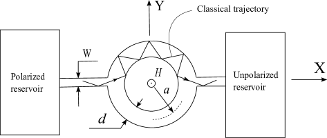
Figure 1: Geometry of the problem under consideration. The $Z$-axis points to the reader. $W$ is the leads width, $d~{}$is the ring arms width, and $a$ is the radius of the ring.

$$\delta H_{Z}=\frac{\hbar\omega_{H}}{2}\,\sigma_{z}\,,\hphantom{w}\omega_{H}=\frac{g}{2}\frac{|e|H}{m^{*}c}\,,$$ (1)

where $e$ is the electron charge, $H$ is the magnetic field, $g$ is the g-factor, $m^{*}$ is the effective electron mass, and $c$ is the light velocity.

The Rashba spin-orbit interaction is assumed to take place only in the range of the ring. It has the form

$$\delta H_{R}=\alpha_{so}\,\hat{\bm{\sigma}}\cdot[\hat{{\mathbf{p}}}\times{\mathbf{z}}]\,.$$ (2)

Here $\alpha_{so}$ is the SOI constant, the vector $\hat{\bm{\sigma}}$ consists of the Pauli matrices $\hat{\sigma}_{x}$, $\hat{\sigma}_{y}$ and $\hat{\sigma}_{z}$, $\hat{\mathbf{p}}$ is the momentum operator and ${\mathbf{z}}$ is a unit vector parallel to the $Z$-axis. We assume the hard wall reflection of electrons from the ring boundaries. Since the particle spin is conserved upon such a reflection, Eqs. (1) and (2) determine a spin dynamics in the ring.

The reservoirs are assumed to be in a local thermodynamic equilibrium with a given polarization (magnetization). For simplicity we assume that the left reservoir is polarized (along a unit vector $\bm{\nu}$), while the right one is unpolarized. The polarization of the left reservoir is characterized by the chemical potentials $\mu_{L\uparrow}=\mu_{L}+\frac{\delta\mu}{2}$ and $\mu_{L\downarrow}=\mu_{L}-\frac{\delta\mu}{2}$, for spin-up and spin-down (relative to $\bm{\nu}$) electrons, respectively. For the right reservoir we assume, in its turn, that $\mu_{R\uparrow}=\mu_{R\downarrow}=\mu_{L}$. This situation is of particular interest for our further analysis, because establishing of thermodynamic equilibrium between spin subsystems in the reservoirs will be accompanied by the spin current, while the electric current will be absent. In the linear response regime the spin current in the right lead can be expressed (see Appendix A) as

$$J_{j}=\sum_{i}g_{ji}\nu_{i}\delta\mu\,,$$ (3)

where $i$ and $j$ take the values $x,y,z$, and $\nu_{j}$ is the $j$-th component of $\bm{\nu}$.

III Semiclassical approximation

We assume that the leads connecting the ring with reservoirs are ideal conductors with a constant cross section. This suggests the use of the Landauer approach for calculation of the spin current. The latter, however, has an important distinction from the electric current, because it does not conserve in the region with SO interaction. Let us assume, for example, that such a region is ideally transparent. Even in this case the transmitted spin current will not be equal to the incident one. Alternatively, we may consider a polarized reservoir connected via one lead to a region with SO interaction. In the stationary case the electric current through this lead will be zero. At the same time , the spin current will be finite, because spin polarizations of incident and reflected electrons can be different. This sort of spin transport has been considered in Ref. Malsh, where a ring played the role of the region with SO interaction.

So, we see that Landauer formula should be modified to take into account effects of nonconcerving spin. In general case it is done in Appendix A. For a particular set up considered in this work the expression for the spin conductance takes a simple form, somewhat similar to the Landauer formula

$$g_{ji}=\frac{1}{4\pi\hbar}\sum_{pp^{\prime}}{\rm Tr}\left\{\hat{t}_{p^{\prime}p}^{\,+}(\mu_{R})\,\hat{\sigma_{j}}\,\hat{t}_{p^{\prime}p}(\mu_{R})\,\hat{\sigma_{i}}\right\}$$ (4)

Here $\hat{t}_{p^{\prime}p}(\mu_{R})$ is the $2\times 2$ matrix composed of the transmission amplitudes $t_{p^{\prime}p}^{\uparrow\uparrow}(\mu_{R})$,$\,t_{p^{\prime}p}^{\uparrow\downarrow}(\mu_{R})\,$, $t_{p^{\prime}p}^{\downarrow\uparrow}(\mu_{R})\,$, $t_{p^{\prime}p}^{\downarrow\downarrow}(\mu_{R})\,$ from the channel $p$ of the left lead to the channel $p^{\prime}$ of the right lead. The summation is performed over open channels. Note, that this formula implies that for calculation of all spin conductance components it is not sufficient to calculate the spin-resolved transmission coefficients $T^{\alpha^{\prime}\alpha}\equiv\sum_{p^{\prime}p}|t_{p^{\prime}p}^{\alpha^{\prime}\alpha}|^{2}$ (studied, for example, in Refs. Frustaglia, ; Frustaglia_2, ). This is readily seen, for example, by inspecting the expression

$$g_{xz}=\frac{1}{4\pi\hbar}\sum_{pp^{\prime}}\left\{(t_{p^{\prime}p}^{\downarrow\uparrow})^{*}\,t_{p^{\prime}p}^{\uparrow\uparrow}-(t_{p^{\prime}p}^{\uparrow\downarrow})^{*}\,t_{p^{\prime}p}^{\downarrow\downarrow}\right\},$$

which follows from (4).

To find the transmission amplitudes in (4) we will follow Ref. FL, (see also Ref. Kaw, ) for the spinless transmission amplitude at the Fermi energy $E_{F}$. In the presence of spin degrees of freedom it allows the evident generalization:

$$t^{\alpha^{\prime}\alpha}_{p^{\prime}p}=-i\hbar\sqrt{v_{p^{\prime}}v_{p}}\int dydy^{\prime}u_{p^{\prime}}^{*}(y^{\prime})u_{p}(y)G(y^{\prime}\alpha^{\prime},y\alpha|E_{F})\,.$$ (5)

$v_{p^{\prime}}$ ($v_{p}$) is the longitudinal velocity in the $p^{\prime}$-th ($p$-th) channel of the right (left) lead. $G$ is the retarded Green’s function. The integration is performed over cross-sections of the leads. We assume that the leads and ring arms are wide enough, so that there are many channels below the Fermi energy. This allows to apply the semiclassical approximation (see e.g. Ref. JBS_chaos, ) to Eq. (5). Within this approximation the path integral expression for the Green’s function is replaced by the sum of amplitudes corresponding to classical trajectories traversing the ring (details of this procedure may be found in Ref. Gutz, ). Integration over $y$ and $y^{\prime}$ is performed by the stationary phase method (large parameter in the exponent is the number of open channels in the leads). The result is

$$t^{\alpha^{\prime}\alpha}_{p^{\prime}p}=\sum_{s}t_{0}(s)S_{s}^{\alpha^{\prime}\alpha}\,.$$ (6)

The label $s$ enumerates the trajectories that enter the ring at the angle $\theta=\pm\sin^{-1}\left(p\pi/k_{F}W\right)$ relative to the $x-$axis and exit it at $\theta^{\prime}=\pm\sin^{-1}\left(p^{\prime}\pi/k_{F}W\right)$, where $W$ and $k_{F}$ are the leads width and Fermi wave number, respectively. $t_{0}(s)$ is the spin independent transmission amplitude corresponding to the $s-$th classical trajectory,

$$t_{0}(s)=-\sqrt{\frac{i}{2N_{m}}}\;\mathrm{sgn}\left[\theta_{s}\right]\;\mathrm{sgn}\left[\theta^{\prime}_{s}\right]\sqrt{\tilde{A}_{s}}\\ \times\exp\left\{\vphantom{\oint}ik_{F}L_{s}+ik_{F}\left(\sin\theta_{s}y_{s}-\sin\theta_{s}^{\prime}y^{\prime}_{s}\right)\right.\\ \left.+\frac{ie}{\hbar c}\oint_{s}\bm{A}d\bm{r}-i\tilde{\mu}_{s}\frac{\pi}{2}\right\}\,.$$ (7)

Here $N_{m}\equiv int\{k_{F}W/\pi\}$ is the number of open channels, $L_{s}$ is the length of the $s$-th trajectory, $y_{s}$ ($y_{s}^{\prime}$) stands for the $y$-coordinate of the entrance (exit) point of $s$-th trajectory, $\bm{A}$ is the vector potential corresponding to the magnetic field applied to the ring. Other quantities in (7) are

$$\tilde{A}_{s}=\frac{1}{a\cos\theta_{s}^{\prime}}\left|\frac{\partial y(\theta,\theta^{\prime})}{\partial\theta^{\prime}}\right|\,,$$

$$\tilde{\mu}_{s}=\mu_{s}+\Theta\left[\frac{\partial\theta(y,y^{\prime})}{\partial y}\right]+\Theta\left[-\frac{\partial\theta^{\prime}(\theta,y^{\prime})}{\partial y^{\prime}}\right]\,,$$

where $\mu_{s}$ is the Maslov index JBS_chaos ; Gutz and $\Theta$ is the Heaviside step function. The matrix $S_{s}^{\alpha^{\prime}\alpha}$ in (6) determines an evolution of the spin state along $s$-th trajectory. It should be noted that Eq. (6) has been derived assuming that classical trajectories do not depend on the spin dynamics. This allowed to write the terms entering into the sum in Eq. (6) in the form of a product of spin dependent and spin independent parts. In fact, this assumption means that in the leading semiclassical approximation we ignore a difference between Fermi velocities corresponding to spin-split subbands. It can be done, if during the time between two consecutive collisions with ring boundaries, a divergence of two wave packets belonging to these subbands will be much less than the electron wavelength. The corresponding condition can be written as $L_{SO}=\hbar/\alpha_{SO}\ m^{*}\gg d$ where $L_{SO}$ is the spin-orbit length that measures the SOI strength and $d$ is the ring width.

For a spin dependent Hamiltonian consisting of the two terms represented by Eqs. (2) and (1), the evolution operator can be expressed as

$$\widehat{S}_{s}={\cal T}\left[\exp\left\{-\frac{i}{\hbar}\int dt\,\left(\alpha_{so}p_{F}\,\hat{\bm{\sigma}}\cdot\bm{n}_{t}+\frac{\hbar\,\omega_{H}}{2}\,\hat{\sigma}_{z}\right)\right\}\right]\,.$$ (8)

Here ${\cal T}$ is the time ordering symbol, $p_{F}$ is the Fermi momentum, $\bm{n}_{t}$ is the unit vector parallel to $\mathbf{p}\times\mathbf{z}$, and p ($|\textbf{p}|=p_{F}$) is the electron momentum. Note, that direction $\bm{n}_{t}$ of the effective magnetic field generated by the SO interaction changes its sign when a particle reverses its motion direction.

Substituting (6) into (4) we obtain

$$g_{ji}=\frac{1}{4\pi\hbar}\sum_{p^{\prime},p}\sum_{s,u}t_{0}^{*}(s)t_{0}(u){\rm Tr}\left\{\hat{\sigma}_{i}\widehat{S}_{s}^{+}\hat{\sigma}_{j}\widehat{S}_{u}\right\}\,.$$ (9)

In this equation each semiclassical amplitude $t_{0}(s)$ contains a phase factor $\exp\left\{2\pi iL_{s}/\lambda\right\}$. Since the path lengths $L_{s}$ and $L_{u}$ of trajectories in Eq. (9) are much longer than the electron wavelength $\lambda$, the terms with $s\neq u$ oscillate rapidly even with a small variation of the particle energy, as well as slight change of the loop shape and/or impurity positions. In an experimental situation it can also be gate voltage variations and magnetic field switching Morpurgo . On the other hand, the diagonal terms with $s=u$ do not oscillate. If one is not interested in mesoscopic fluctuations of the spin conductance, or quantum corrections to it, only the terms with $s=u$ have to be retained JBS_Blum_Smil . On the basis of the ergodic hypothesis of Ref. Lee_Stone_Fukuyama, this procedure may also be treated as averaging over a random ensemble of the rings.

Thus, from (9) the averaged spin conductance $\langle g_{ij}\rangle$ is obtained as

$$\langle g_{ij}\rangle=\frac{1}{2\pi\hbar}\sum_{s}|t_{0}(s)|^{2}K_{ij}^{s}\ .$$ (10)

where

$$K_{ij}^{s}=\frac{1}{2}{\rm Tr}\left\{\hat{\sigma}_{i}\widehat{S}_{s}\hat{\sigma}_{j}\widehat{S}_{s}^{{\dagger}}\right\}\ .$$ (11)

The electrical conductance $G$ after such averaging takes the form

$$\langle G\rangle=(e/\pi\hbar)\sum_{s}|t_{0}(s)|^{2}\,,$$ (12)

where the factor $2$ accounts for the spin degrees of freedom. It should be noted that $\langle G\rangle$ given by (12) does not depend on the SO interaction strength. On the other hand, oscillations of $G$ with the varying Rashba constant have been predicted in Ref. Aronov_LG, . This distinction can be explained by importance of quantum effects in an ideal 1D ring considered in Ref. Aronov_LG, , while such effects are small in a disordered multichannel system that we study here. They can be taken into account as weak localization corrections to AC oscillations similar to those studied for diffusive rings. Mathur

Let us now consider the transparency

$$N=\sum_{p^{\prime},p}\left|\,t_{p^{\prime}p}\,\right|^{2}$$

for a spinless particle. Here $t_{p^{\prime}p}$ is the transmission amplitude from the channel $p$ on the left to the channel $p^{\prime}$ on the right. So, the transparency $N$ is normalized to the number of open channels $N_{m}$. Applying configurational averaging to the above expression we obtain it as a sum over trajectories:

$$\langle N\rangle=N_{cl}\equiv\sum_{s}\left|t_{0}(s)\right|^{2}\,.$$ (13)

Hence, the ratio

$$P(s)=\frac{\left|t_{0}(s)\right|^{2}}{N_{cl}}$$

can be identified with the probability that an electron chooses the $s$-th trajectory to pass the ring. Expressing $\left|t_{0}(s)\right|^{2}$ from the last formula and substituting it into (10) we obtain

$$\langle g_{ij}\rangle=g_{0}\langle K_{ij}^{s}\rangle_{s}\,,$$ (14)

where $\langle\cdot\rangle_{s}$ denotes averaging over trajectories with the probability $P(s)$ and $2e^{2}g_{0}=e^{2}N_{cl}/\pi\hbar$ is a classical conductance of the ring Kaw .

We assume that the classical motion of an electron inside the ring is chaotic. The chaotic dynamics is provided by small scale bumps and other irregularities on the ring boundaries, while macroscopically the ring preserves its regular shape. For chaotic trajectories after long enough time an electron ”forgets” through which of the leads it entered the ring. Together with an assumption that the leads are symmetric this allows to conclude that probability for a particle to be reflected is equal to the probability to be transmitted. So, $N_{cl}=N_{m}/2$ and $g_{0}=N_{m}/4\pi\hbar$.

Formula (14) will be used for calculation of the spin conductance $\langle g_{ij}\rangle$. However, another physically more transparent representation of $\langle g_{ij}\rangle$ can be suggested. As shown in Appendix B, $K_{ij}^{s}$is the $i$-th component of the electron polarization at the end of the $s$-th trajectory, provided that at its beginning the electron was polarized along the $j$-th axis. Taking this into account one can introduce the effective polarization vector $\bm{P}_{eff}(s|\bm{e}_{j})\equiv\left[g(s)/g_{0}\right]\left\{K_{xj}^{s},K_{yj}^{s},K_{zj}^{s}\right\}$ of electrons at the end of the $s$-th trajectory. Here $g(s)=\left|t_{0}(s)\right|^{2}/2\pi\hbar$ is the flux of spinless particles that pass the ring through the $s$-th trajectory. Eq. (10) then takes the form

$$\langle g_{ij}\rangle=g_{0}\sum_{s}P^{i}_{eff}(s|\bm{e}_{j})\,.$$ (15)

From comparison of (14) and (15) we see that $\langle K_{ij}^{s}\rangle_{s}$ may be treated as $i$-th component of the effective polarization vector $\bm{P}_{eff}(\bm{e}_{j})$ on the exit from the ring,

$$\langle K_{ij}^{s}\rangle_{s}=P^{i}_{eff}(\bm{e}_{j})\equiv\sum_{s}P^{i}_{eff}(s|\bm{e}_{j})\,.$$ (16)

Equation (15) means that the spin current on the exit from the ring is given by the sum of effective polarizations corresponding to each classical trajectory, times the flux of particles passing the ring. From this fact an immediate conclusion follows: if the resonance condition is satisfied, that is the effective polarizations corresponding to different trajectories on the exit from the ring are co-directional, then the spin current will have a maximum.

IV Fokker-Planck equation

According to Eq. (14) calculation of the spin conductance $\langle g_{ij}\rangle$ reduces to averaging of the polarization transformation matrix $K_{ij}^{s}$ over trajectories. To perform this averaging the distribution function of $K_{ij}^{s}$ is needed. One of the standard ways to find it is the following. We note that the quantities $K_{ij}^{s}$ in (11) correspond to the end of the $s$-th trajectory. It is evident however that one may extend definition (11) to any time instant $t$ on the trajectory. Taking then a time derivative of (11) we arrive at the stochastic differential equation (of the Langevin type) for $K_{ij}^{s}$. This equation may be used to calculate drift and diffusion coefficients in the Fokker-Planck equation. Solving then this Fokker-Planck equation one can find the desired distribution function.

IV.1 Dynamical equation for the spin S-matrix along a trajectory

As a preparation step to our calculation we note that at $H=0$ eq. (8) for $\widehat{S}_{s}$ can be written in the form of a contour integral over the $s$-th trajectory:

$$\widehat{S}_{s}(H=0)={\cal T}\left[\exp\left\{-\frac{i}{L_{SO}}\oint_{s}d{\bm{l}}\,\cdot\left[\bm{z}\times\hat{\bm{\sigma}}\right]\right\}\right]\,,$$ (17)

As any unitary operator acting in the spin space, $S_{s}(H=0)$ can also be written in the form of the rotation operator

$$\widehat{S}_{s}(H=0)=\exp\left\{i\frac{\hat{\sigma}_{\bm{N}}\Psi}{2}\right\}\,,$$ (18)

where $\hat{\sigma}_{\bm{N}}$ is a projection of $\hat{\bm{\sigma}}$ onto some unit vector $\bm{N}$. An important consequence of (17) is that $\bm{N}$ and $\Psi$ depend only on the geometry of the $s$-th trajectory and don’t depend on the dynamics of motion along the trajectory. This is the reason why $\Psi$ may be called a geometric phaseMalsh .

To extend the analysis of Ref. Malsh, and take into account finiteness of the ring width we divide the time interval $(0,t)$ into small subintervals $\Delta t_{i}=t_{i}-t_{i-1};\,t_{0}=0<t_{1}<\dots<t_{n}=t$. After that $\widehat{S}$ can be represented in the form (the index $s$ is omitted when it doesn’t lead to any confusion)

$$\widehat{S}(t)=\widehat{S}(\Delta t_{n})\widehat{S}(\Delta t_{n-1})\dots\widehat{S}(\Delta t_{1})\,.$$ (19)

The real trajectory is transformed next by adding to each i-th segment a path passed in direct and opposite directions, as shown in Fig. 2. It is seen from (17), that paths passed twice in the opposite directions don’t contribute to $\widehat{S}_{s}(H=0)$. Consequently, each term $\widehat{S}(\Delta t_{i})$ in (19) may be replaced without changing $\widehat{S}_{s}$ with

$$\widehat{S}_{\bm{abc}}\equiv\widehat{S}_{\bm{c}}(H=0)\widehat{S}_{\bm{b}}\widehat{S}_{\bm{a}}(H=0)\,.$$ (20)

Here $\bm{b}$ is the trajectory segment corresponding to the time interval $\Delta t_{i}$, $\bm{a}$ and $\bm{c}$ connect the middle line of the ring with $\bm{b}$, as explained in Fig. 2.

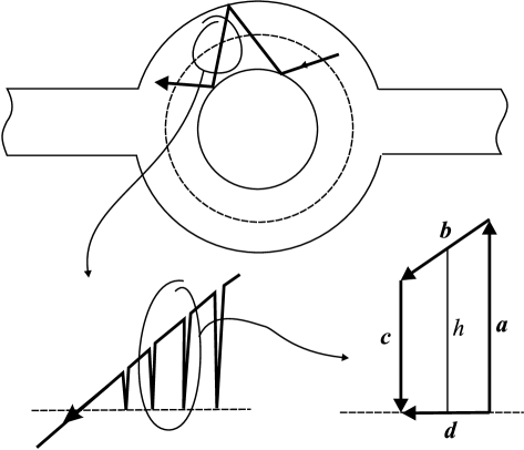
Figure 2: Replacement of the real trajectory with the fictitious one in the case of the ring of finite width. Both trajectories give rise to the same evolution operator $S_{s}$ in the absence of the magnetic field.

Expanding exponents in (8) and (17) one obtains

$$\widehat{S}_{\bm{abc}}=1-\frac{i}{L_{SO}}\hat{\sigma}_{r}dl-i\frac{\omega_{H}}{2}\hat{\sigma}_{z}\Delta t_{i}+2\frac{i}{L_{SO}^{2}}\hat{\sigma}_{z}\Sigma_{\bm{abc,-d}}\,,$$ (21)

where $dl=|\bm{d}|$ for counterclockwise rotation of the electron and $dl=-|\bm{d}|$ otherwise. $\hat{\sigma}_{r}$ is the projection of $\hat{\bm{\sigma}}$ on the radius vector. $\Sigma_{\bm{abc,-d}}$ is the oriented area of the trapezium formed by the vectors $\bm{a,b,c}$ and $\bm{-d}$. It is positive if the contour $\bm{abc,-d}$ is positively oriented and negative otherwise. The last term in (21) takes into account the finite width of the ring. It leads to a phase proportional to the area embraced by the trajectory, analogously to the finite width effect on the Aharonov-Bom phaseKaw_Nak .

Formulae (19) and (21) yield the following dynamical equation for the spin evolution operator

$$\frac{\partial\widehat{S}}{\partial t}=\left\{i\gamma\dot{\phi}\left(e^{i\phi}\hat{\sigma}_{-}+e^{-i\phi}\hat{\sigma}_{+}\right)-i\eta\hat{\sigma}_{z}\right\}\widehat{S}\,.$$ (22)

Here

$$\gamma=a/L_{SO}\,,$$ (23)

$$\hat{\sigma}_{\pm}=\frac{\hat{\sigma}_{x}\pm i\hat{\sigma}_{y}}{2}\,,$$

$$\eta\equiv\eta(t)=\frac{\omega_{H}}{2}-2\gamma^{2}\frac{h(t)}{a}\dot{\phi}\,,$$ (24)

$a$ is the ring radius (distance from the center to the middle line of the ring), and $\dot{\phi}$ is the time derivative of the polar angle $\phi$ counted from the negative direction of the $OX$-axis. The deviation $h(t)$ of the electron trajectory from the middle line (see Fig. 2) is taken positive for points outside the circle formed by this line and negative otherwise.

Dynamical equation (22) simplifies if we change the system of coordinates. First we perform transformation to the system $\widetilde{OXYZ}$ rotating together with the electron ($\widetilde{OZ}$-axis coincides with the $OZ$-axis, $\widetilde{OX}$ and $\widetilde{OY}$ axes rotate with the angular velocity $\dot{\phi}$ around $OZ$-axis). In this system the evolution operator takes the form

$$\widetilde{S}=\widehat{R}_{z}(t)\widehat{S}\widehat{R}^{-1}_{z}(0)\,,$$ (25)

$$\widehat{R}_{z}(t)=\exp\left\{i\hat{\sigma}_{z}\phi(t)/2\right\}\,.$$ (26)

Using (22) and (25) and taking into account that $\widehat{R}^{-1}_{z}(0)=1$ one can verify that $\widetilde{S}$ satisfies the equation

$$\frac{d\,\widetilde{S}}{d\,t}=\left\{-i\frac{\hat{\sigma}_{\theta}\omega_{0}}{2}-i\eta\hat{\sigma}_{z}\right\}\widetilde{S}\,,$$ (27)

where $\hat{\sigma}_{\theta}$ is a projection of $\hat{\bm{\sigma}}$ onto the vector

$$\bm{\theta}=\left\{2\gamma/\zeta,0,1/\zeta\right\}\,,$$ (28)

$$\zeta=\sqrt{1+4\gamma^{2}}\,,$$ (29)

and

$$\omega_{0}=-\zeta\dot{\phi}\,.$$ (30)

Next, we rotate $\widetilde{OXYZ}$ around $\widetilde{OY}$-axis,until $\widetilde{OZ}$ comes parallel to $\bm{\theta}$. The new coordinate system denoted as $\widetilde{OX^{\prime}YZ^{\prime}}$ will be called below the tilted rotating (TR) system. In TR coordinates the evolution operator takes the form

$$\widetilde{S^{\prime}}=\widehat{R}_{y}\widetilde{S}\widehat{R}_{y}^{-1}=\widehat{R}_{y}\widehat{R}_{z}\widehat{S}\widehat{R}_{y}^{-1}$$ (31)

$$\widehat{R}_{y}=\exp\left\{i\hat{\sigma}_{y}\chi_{0}/2\right\}\,.$$

The angle $\chi_{0}$ between $\widetilde{OZ}$ and $\widetilde{OZ^{\prime}}$ is defined by the relations

$$\cos\chi_{0}=1/\zeta,\,\sin\chi_{0}=2\gamma/\zeta\,.$$ (32)

The evolution of $\widetilde{S^{\prime}}$ is determined by

$$\frac{d\,\widetilde{S^{\prime}}}{d\,t}=i\frac{\hat{\bm{\sigma}}\bm{\Omega}}{2}\widetilde{S^{\prime}}$$ (33)

$$\bm{\Omega}\equiv\left\{\frac{4\gamma}{\zeta}\eta,\,0,\,-\omega_{0}-\frac{2\eta}{\zeta}\right\}\,.$$ (34)

The physical meaning of the TR system is rather transparent. At vanishing ring width and zero magnetic field this is the coordinate system where the effective magnetic field produced by the Rashba SOI is parallel to the $\widetilde{OZ^{\prime}}$-axis.

IV.2 Evolution of spin state along a trajectory in terms of polarization vector

Transition from $\widehat{S}$ in (11) to $\widetilde{S^{\prime}}$ yields

$$K_{ij}=\frac{1}{2}{\rm Tr}\left\{\widetilde{\sigma}^{\prime}_{i}\,\widetilde{[\sigma_{j}(t)]}^{\prime}\right\}\,,$$ (35)

where

$$\widetilde{\sigma}^{\prime}_{i}=\widehat{R}_{y}\widehat{R}_{z}\hat{\sigma}_{i}\widehat{R}_{z}^{+}\widehat{R}_{y}^{+}\,,$$ (36)

$$\widetilde{[\sigma_{j}(t)]}^{\prime}=\widetilde{S^{\prime}}\hat{\sigma}^{\prime}_{j}\widetilde{S^{\prime}}^{+}=\widehat{R}_{y}\widehat{R}_{z}\hat{\sigma}_{j}(t)\widehat{R}_{z}^{+}\widehat{R}_{y}^{+}\,,$$ (37)

$$\hat{\sigma}_{j}^{\prime}=\widehat{R}_{y}\hat{\sigma}_{j}\widehat{R}_{y}^{-1}=\left.\tilde{\sigma}_{j}^{\prime}\right|_{t=0}\,,$$

$$\hat{\sigma}_{j}(t)=\widehat{S}\hat{\sigma}_{j}\widehat{S}^{+}\,.$$

It is easy to see that $\widetilde{\sigma}^{\prime}_{i}$ in (36) is an image of $\hat{\sigma}_{i}$ after transformation to the TR coordinates. Analogously, $\widetilde{[\sigma_{j}(t)]}^{\prime}$ is is an image of $\hat{\sigma}_{j}(t)$ after the same transformation. Note, that both $\widetilde{\sigma}^{\prime}_{i}$ and $\widetilde{[\sigma_{j}(t)]}^{\prime}$ depend on time: $\widetilde{\sigma}^{\prime}_{i}$ — due to rotation of the TR system of coordinates, $\widetilde{[\sigma_{j}(t)]}^{\prime}$ — due to rotation of the electron spin (described by the evolution operator) and rotation of the TR system of coordinates. Further, both $\widetilde{\sigma}^{\prime}_{i}$ and $\widetilde{[\sigma_{j}(t)]}^{\prime}$ can be decomposed into the sums over $\hat{\sigma}_{p}$,

$$\widetilde{\sigma}^{\prime}_{i}=\sum_{p=1}^{3}\Lambda^{0}_{pi}\hat{\sigma}_{p}\,$$ (38)

$$\widetilde{[\sigma_{j}(t)]}^{\prime}=\sum_{p=1}^{3}\Lambda_{pj}\hat{\sigma}_{p}\,.$$ (39)

The superscript $"0"$ at $\Lambda_{pi}$ in (38) indicates, that $\Lambda_{pi}$ transforms into $\Lambda^{0}_{pi}$ with $\alpha_{so}\longrightarrow 0$. The unit matrix $\hat{\sigma}_{0}$ is not present in these sums because the traces of $\widetilde{\sigma}^{\prime}_{i}$ and $\widetilde{[\sigma_{j}(t)]}^{\prime}$ are zero, as can be seen from (36) and (37). Using (117) from Appendix B one can check, that $\Lambda_{pj}$ are TR coordinates of the electron spin, provided that the initial spin was $\bm{e}_{j}$. Analogously, $\Lambda^{0}_{pi}$ are coordinates of $\bm{e}_{i}$ in the TR system. After substitution into (35) the sums (38) and (39) lead to $K_{ij}$ written in the form of scalar product,

$$K_{ij}=\bm{\Lambda}^{0}_{i}\cdot\bm{\Lambda}_{j}\,,$$ (40)

$$\bm{\Lambda}^{0}_{i}\equiv\left\{\Lambda^{0}_{1i},\Lambda^{0}_{2i},\Lambda^{0}_{3i}\right\}\,,$$

$$\bm{\Lambda}_{j}\equiv\left\{\Lambda_{1j},\Lambda_{2j},\Lambda_{3j}\right\}\,.$$

The components of $\bm{\Lambda}^{0}_{i}$ in (40) being the coordinates of $\bm{e}_{i}$ in the TR system are defined only by its orientation with respect to the original system, that is by the angles $\phi$ and $\chi_{0}$. The angle $\phi$ at the end of the trajectory is $\phi=\pi+2\pi n$, where $n=\pm 1,\pm 2...$ is the winding number. The angle $\chi_{0}$ is also fixed, see (32). Hence, components of $\bm{\Lambda}^{0}_{i}$ at the end of a trajectory are constants defined explicitly by Eq. (36):

$$\bm{\Lambda}^{0}_{x}=\left\{-\frac{1}{\zeta},0,-\frac{2\gamma}{\zeta}\right\}\,,$$ (41a)

$$\bm{\Lambda}^{0}_{y}=\left\{0,-1,0\right\}\,,$$ (41b)

$$\bm{\Lambda}^{0}_{z}=\left\{-\frac{2\gamma}{\zeta},0,\frac{1}{\zeta}\right\}\,.$$ (41c)

With constant $\bm{\Lambda}^{0}_{i}$ averaging of $K_{ij}$ over trajectories reduces to averaging of $\bm{\Lambda}_{j}$. We shall perform this averaging with the use of the distribution function $\cal P$ of $\bm{\Lambda}_{j}$. This function will be obtained from the Fokker-Planck equation which will be derived and solved below.

The equation of motion for $\widetilde{[\sigma_{j}(t)]}^{\prime}$ is found from (37) and (33). In view of the expansion (39) it can be written as an equation of motion for $\bm{\Lambda}_{j}$:

$$\frac{d\bm{\Lambda}_{j}}{d\,t}=\left[\bm{\Lambda}_{j}\times\bm{\Omega}\right]\,.$$ (42)

This equation should be supplemented with the initial conditions

$$\left.\bm{\Lambda}_{x}\right|_{t=o}=\left\{1/\zeta,\,0,\,2\gamma/\zeta\right\}\,,$$ (43a)

$$\left.\bm{\Lambda}_{y}\right|_{t=o}=\left\{0,\,1,\,0\right\}\,,$$ (43b)

$$\left.\bm{\Lambda}_{z}\right|_{t=o}=\left\{-2\gamma/\zeta,\,0,\,1/\zeta\right\}\,,$$ (43c)

which can be derived from (37) and (39).

IV.3 Stochastic differential equations for the angles determining the position of an electron and direction of its spin polarization

It follows from (39) that $\bm{\Lambda}_{j}^{2}={\rm Tr}\left\{\widetilde{[\sigma_{j}(t)]}^{\prime\,2}\right\}/2=1$. This allows to describe $\bm{\Lambda}_{j}$ by only two variables, the polar angle $\Phi$ and azimuthal angle $\Theta$. Eq.(42) is then reduced to

$$\left\{\begin{array}[]{rl}\dot{\Theta}&=\frac{4\gamma}{\zeta}\eta\sin\Phi\\ \dot{\Phi}&=\omega_{0}(t)+\frac{2}{\zeta}\eta\left[1+2\gamma\cos\Phi\cot\Theta\right]\,.\end{array}\right.$$

It is convenient to represent the angle $\Phi$ in the form $\Phi=\psi+\delta$, where

$$\psi\equiv-\zeta\phi\,.$$ (44)

For these new variables we obtain the system of equations:

$$\left\{\begin{array}[]{rl}\dot{\Theta}&=2\gamma\left(\frac{\omega_{H}}{\zeta}+\omega_{W}(t)\right)\sin(\psi+\delta)\\ \dot{\delta}&=\left(\frac{\omega_{H}}{\zeta}+\omega_{W}(t)\right)\left[1+2\gamma\cos(\psi+\delta)\cot\Theta\right]\\ \dot{\psi}&=\omega_{0}(t)\,,\end{array}\right.$$ (45)

where we have introduced the frequency $\omega_{W}$ associated with the finite width of the ring,

$$\omega_{W}(t)=\mu(t)\omega_{0}(t),\,\mu(t)=\left(\frac{2\gamma}{\zeta}\right)^{2}\frac{h(t)}{a}\,.$$ (46)

At the weak enough magnetic field $\omega_{H}\ll\omega_{0}$. If, in addition, the ring is narrow, $h(t)\ll a$, then $\mu(t)\ll 1$ and $\omega_{W}\ll\omega_{0}$, as follows from (46). Returning to (45) we thus see that $\Theta$ and $\delta$ are ”slow” variables, while $\psi$ is a ”fast” variable. Such a separation of variables simplifies considerably the Fokker-Planck equation, which will be derived below from the system of stochastic differential equations (45).

IV.4 Derivation of the Fokker-Planck equation

Parameters of the Fokker-Planck equation for the distribution function ${\cal P}(\Theta,\delta,\psi)$ are determined by the drift $A_{\Theta}$, $A_{\delta}$, $A_{\psi}$ and diffusion $B_{ij};\,i,j=\left\{\Theta,\delta,\psi\right\}$ coefficients Drift_Diffus . Let us first consider the diffusion coefficient $B_{\psi\psi}$ given by

$$B_{\psi\psi}=\lim_{\Delta t\rightarrow 0}\frac{\overline{\left(\Delta\psi\right)^{2}}}{\Delta t}\,,$$ (47)

where $\Delta\psi$ is the increment of the stochastic process $\psi(t)$. It follows from Eq. (44) that $\overline{(\Delta\psi)^{2}}=\zeta^{2}\overline{(\Delta\phi)^{2}}$. On the other hand,it was shown in Ref. Berry_Robnik, that the winding number $w$ of the classically chaotic trajectories has a Gaussian distribution

$${\cal P}\left(w\left|T\right.\right)=\left(2\pi T/T_{1}\right)^{-1/2}\exp\left\{\frac{-w^{2}}{2T/T_{1}}\right\}.$$ (48)

where the constant $T_{1}$ is the characteristic time of one turn, $\langle w^{2}(T_{1})\rangle=1$. This equation means that the winding of trajectories is a diffusion process. One can extend (48) to a range of $w=\phi/2\pi<1$ assuming that a particle advances diffusively along a ring arm. Such situation takes place if the rotation direction $\dot{\phi}/|\dot{\phi}|$ changes many times, while passing the angular distance $\Delta\phi<2\pi$. Moreover, the angular distance between two consecutive changes of a rotation direction must be small enough to ensure a small change of $\Phi$ and $\psi$. Hence, as follows from Eq. (44) this distance must be $\ll\zeta^{-1}$. We assume that scattering from ring boundaries and spatially fluctuating potential make this condition satisfied.

From (47) and (48) with $w=\phi/2\pi$ we immediately find

$$B_{\psi\psi}\equiv\lim_{\Delta t\rightarrow 0}\frac{\overline{\left(\Delta\psi\right)^{2}}}{\Delta t}=\frac{\left(2\pi\zeta\right)^{2}}{T_{1}}\,,$$ (49)

where the overline denotes averaging over trajectories. Other diffusion coefficients, as well as drift coefficients, are conveniently expressed in terms of the diffusion coefficient of the auxiliary stochastic processes $u(t)$, which is defined by its stochastic differential

$$du=\omega_{W}(t)dt\,.$$ (50)

An assumption that the deviation $h(t)$ of a trajectory from the middle line of the ring and the angle $\phi$ fluctuate independently leads to the absence of correlations between the stochastic processes $\psi(t)$ and $u(t)$. Assuming also a uniform distribution of $h$ over the width $d$ of the ring arms, we find from Eq. (46)

$$B_{u\psi}=B_{\psi u}\equiv\lim_{\Delta t\rightarrow 0}\frac{\overline{\Delta\psi\,\Delta u}}{\Delta t}=0\,,$$ (51)

$$B_{uu}\equiv\lim_{\Delta t\rightarrow 0}\frac{\overline{\left(\Delta u\right)^{2}}}{\Delta t}=\left(\frac{2\gamma}{\zeta}\right)^{4}\frac{d^{\,2}}{12a^{2}}B_{\psi\psi}\,.$$ (52)

Further, Eq. (45) can be used to express the small increments $\Delta\Theta,\Delta\delta,\Delta\psi$ in the form of integrals over time interval $\Delta t$. Then, after averaging procedure the limits $\Delta t\rightarrow 0$ must be taken. For example, $A_{\Theta}=\lim_{\Delta t\rightarrow 0}\overline{\Delta\Theta}/\Delta t,\,B_{\Theta\delta}=\lim_{\Delta t\rightarrow 0}\overline{\Delta\Theta\,\Delta\delta}/\Delta t$. We thus obtain

$$\left\{\begin{array}[]{l}A_{\Theta}=\omega_{H}\frac{2\gamma}{\zeta}\sin\left(\psi+\delta\right)+\frac{B_{uu}}{2}2\gamma\cos\left(\psi+\delta\right)F\,,\\ A_{\psi}=0\,,\\ A_{\delta}=\frac{\omega_{H}}{\zeta}F-\frac{B_{uu}}{2}2\gamma\sin\left(\psi+\delta\right)\left[cot\Theta\right.\\ \left.\phantom{aaaaaaaaaaaaaaaa}+2\gamma\frac{\cos^{2}\Theta+1}{\sin^{2}\Theta}\cos\left(\psi+\delta\right)\right]\,,\end{array}\right.$$ (53)

$$\left\{\begin{array}[]{l}B_{\Theta\Theta}=\sin^{2}(\psi+\delta)(2\gamma)^{2}B_{uu}\,,\\ B_{\delta\delta}=F^{2}B_{uu}\,,\\ B_{\Theta\delta}=2\gamma\sin\left(\psi+\delta\right)FB_{uu}\,,\\ B_{\psi\Theta}=B_{\psi\delta}=0\,,\end{array}\right.$$ (54)

where

$$F=1+2\gamma\cos(\psi+\delta)\cot\Theta\,.$$

These coefficients should be inserted in the Fokker-Planck equation

$$\frac{\partial}{\partial t}\left({\cal P}\sin\Theta\right)=\\ -\sum_{i}\frac{\partial}{\partial x_{i}}\left(A_{x_{i}}{\cal P}\sin\Theta\right)+\frac{1}{2}\sum_{i,\,j}\frac{\partial^{2}}{\partial x_{i}\partial x_{j}}\left(B_{x_{i}\,x_{j}}{\cal P}\sin\Theta\right)\,,$$

where the variables $x_{i}\>(i=1,2,3)$ denote $\Theta,\,\delta,\,\psi$. The probability density $\cal P$ is normalized in such a way that an integral of ${\cal P}\sin\Theta$ over $\Theta,\delta$ and $\psi$ is 1. In this way we arrive at the following equation

$$\sin\Theta\frac{\partial{\cal P}}{\partial t}=\frac{B_{uu}}{2}(2\gamma)^{2}\frac{1}{\sin\Theta}\frac{1+\cos\left[2(\psi+\delta)\right]}{2}{\cal P}\\ -\omega_{H}\frac{2\gamma}{\zeta}\sin(\psi+\delta)\left(\frac{\partial{\cal P}}{\partial\Theta}\sin\Theta+{\cal P}\cos\Theta\right)+\dots{\\ }+\frac{B_{\psi\psi}}{2}\sin\Theta\frac{\partial^{\,2}{\cal P}}{\partial\psi^{\,2}}\,,$$ (55)

where the dots stand for other terms that are proportional to $B_{uu}$ or $\omega_{H}$. All the terms in r.h.s, except for the last one, do not contain derivatives over ${\psi}$. For a narrow enough ring and weak magnetic field, $B_{uu}$ and $\omega_{H}\ll B_{\psi\psi}$. So, diffusion in the space of the ”slow” variables $\Theta$ and $\delta$ is indeed slower than diffusion through the ”fast” variable $\psi$. Hence, the diffusion equation can be averaged over the fast variable. After averaging (55) over $\psi$ we arrive at the Fokker-Planck equation of the form

$$\frac{\partial{\cal P}}{\partial t}=-\frac{\omega_{H}}{\zeta}\frac{\partial{\cal P}}{\partial\delta}+B_{uu}\gamma^{2}\frac{1}{\sin\Theta}\frac{\partial}{\partial\Theta}\left(\sin\Theta\frac{\partial{\cal P}}{\partial\Theta}\right)\\ +B_{uu}\left(\frac{1}{2}+\gamma^{2}cot^{2}\Theta\right)\frac{\partial^{2}{\cal P}}{\partial\delta^{2}}+\frac{B_{\psi\psi}}{2}\frac{\partial^{2}{\cal P}}{\partial\psi^{2}}\,.$$ (56)

This equation should be solved together with the initial conditions for each of the vectors $\bm{\Lambda}_{j}$.

$${\cal P}(\Theta,\psi,\delta|t=0)=\delta(\cos\Theta-\cos\Theta_{0}^{j})\delta(\delta-\delta_{0}^{j})\delta(\psi)\,,$$ (57)

where the angles $\Theta_{0}^{j}$, $\delta_{0}^{j}$ defining the initial positions of the vectors $\bm{\Lambda}_{j}$ are found from (43). Using Eq.(32) $\theta_{0}$ and $\delta_{0}$ can be expressed in terms of $\chi_{0}$. The initial value of $\psi$ should be zero since it is proportional to the initial value of $\phi$, which is zero.

IV.5 Solution of the Focker-Plank equation

After Laplace transformation with respect to time and Fourier transformation with respect to $\delta$ and $\psi$ the equation (56) is reduced to the ordinary differential equation

$$\lambda v-\left\{\frac{1}{\sin\Theta}\frac{\partial}{\partial\Theta}\left(\sin\Theta\frac{\partial}{\partial\Theta}\right)-\frac{\kappa^{2}}{\sin^{2}\Theta}\right\}v\\ =\delta\left(\cos\Theta-\cos\Theta_{0}^{j}\right)\,,$$ (58)

where

$$v=\gamma^{2}B_{uu}e^{i\kappa\delta_{0}^{j}}\tilde{\cal P}\,,$$

$$\tilde{\cal P}\equiv\tilde{\cal P}(\Theta,\kappa,q|p)=\int d\psi d\delta\,e^{-i(\kappa\delta+q\psi)}$$

$$\times\int_{0}^{+\infty}dt\,e^{-p\,t}{\cal P}(\Theta,\delta,\psi|t)\,$$

$$\lambda=\frac{p+i\kappa\frac{\omega_{H}}{\zeta}+\kappa^{2}B_{uu}\left(\frac{1}{2}-\gamma^{2}\right)+q^{2}\frac{B_{\psi\psi}}{2}}{\gamma^{2}B_{uu}}\,.$$

The solution of Eq. (58) can be expressed in terms of eigenfunctions of the linear operator in l.h.s. of this equation. In our case they are the associated Legendre functions $P_{n}^{|\kappa|}(\cos\Theta)$ and we obtain

$${\cal P}(\Theta,\delta,\psi|t)=\frac{e^{-\psi^{2}/(2B_{\psi\psi}t)}}{\sqrt{2\pi B_{\psi\psi}t}}\sum_{\kappa=-\infty}^{+\infty}\frac{e^{ik(\delta-\delta_{0}^{j}-\omega_{H}t/\zeta)}}{2\pi}\\ \times\sum_{n=|\kappa|}^{+\infty}\frac{2n+1}{2}\frac{(n-|\kappa|)!}{(n+|\kappa|)!}P_{n}^{|\kappa|}(\cos\Theta)P_{n}^{|\kappa|}(\cos\Theta_{0}^{j})\\ \times e^{-B_{uu}\left[|\kappa|^{2}\left(\frac{1}{2}-\gamma^{2}\right)+\gamma^{2}n(n+1)\right]t}\,,$$ (59)

In this equation only a factor in front of the first sum depends on $\psi$. It is clear that this factor determines a probability distribution of $\psi$. At the end of trajectories (at the exit from the ring), when $\phi=2\pi w$, $w=\pm 1/2,\pm 3/2...$, it coincides with the winding number distribution (48). The remaining part of (59) is evidently the conditional (for given $\psi$) probability distribution of $\delta$ and $\Theta$. This function can be used for averaging of the polarization vectors $\bm{\Lambda}_{j}$ over trajectories with a given winding number $w$.

IV.6 Averaging of the polarization vectors $\bm{\Lambda_{j}}$

Since the unit vectors $\bm{\Lambda}_{j}$ in Eq. (42) are defined by their respective polar and azimuthal angles $\Theta$ and $\Phi$, one can calculate easily their average values using Eq. (59) and taking into account that $\Phi=\psi+\delta$. We thus arrive at the following expressions for the averages $\langle\bm{\Lambda}_{j}\rangle|_{\psi,T}$ at fixed trajectory duration $T$ and a given $\psi$ (winding number),

$$\langle\Lambda_{xj}\rangle|_{\psi,T}=\sin\Theta_{0}^{j}\cos\left(\psi+\frac{\omega_{H}}{\zeta}T+\delta_{0}^{j}\right)e^{-T/\tau_{\perp}}\,,$$ (60a)

$$\langle\Lambda_{yj}\rangle|_{\psi,T}=\sin\Theta_{0}^{j}\sin\left(\psi+\frac{\omega_{H}}{\zeta}T+\delta_{0}^{j}\right)e^{-T/\tau_{\perp}}\,,$$ (60b)

$$\langle\Lambda_{zj}\rangle|_{\psi,T}=\cos\Theta_{0}^{j}\,e^{-T/\tau_{\|}}\,.$$ (60c)

The parameters $\tau_{\perp}$ and $\tau_{\|}$ have been introduced to characterize relaxation rates of the electron polarization due to the finite width of the ring,

$$\frac{1}{\tau_{\perp}}\equiv\frac{1+\zeta^{2}}{4}B_{ss}\,,$$ (61)

$$\frac{1}{\tau_{\|}}\equiv 2\gamma^{2}B_{ss}\,.$$

As follows from Eq. (60), perpendicular to the $\widetilde{OZ^{\prime}}$-axis components of $\bm{\Lambda}_{j}$ decay with the rate $1/\tau_{\perp}$, while the decay rate of parallel components is $1/\tau_{\|}$. We recall that in the rotating system the direction of the $\widetilde{OZ^{\prime}}$-axis is determined by the vector $\bm{\theta}$, see (28). At $t=0$ the rotating system coincides with the original one. Hence, the electron polarization in the ring relaxes with the rate $\tau_{\perp}$($\tau_{\|}$), if the polarization of the left reservoir is perpendicular (parallel) to $\bm{\theta}$. Besides relaxation associated with finiteness of the ring width, there is an additional relaxation channel due to the magnetic field, that will be discussed below.

To complete calculation of the spin conductance given by Eqs. (14) and (40), the scalar products $\bm{\Lambda}^{0}_{i}\cdot\langle\bm{\Lambda}_{j}\rangle|_{\psi,T}$, where $\bm{\Lambda}^{0}_{i}$ are given by Eq. (41), must be averaged over $\psi$ and $T$. Averaging over $\psi$ is performed with the use of (48), by substituting $w=-\psi/2\pi\zeta$. As for the distribution over $T$, in the case of classically chaotic systems one should use the exponential function JBS_Blum_Smil $\ {\cal P}(T)$=$\tau^{-1}\exp\left\{-(T-T_{0})/\tau\right\}$, where $\tau$ is the mean escape time of a particle and $T_{0}$ is the shortest trajectory duration. The results of calculation for $g_{yy}$, as well as for polarization rotation angles in a magnetic field are shown in Fig. 3 and Fig. 6 respectively. It is seen from these plots that the AC oscillations magnitude and spin rotation angle strongly depend on the parameter $T_{1}/\tau+T_{1}/\tau_{\perp}$, which controls the trajectory winding number during the particle spin lifetime. If this parameter is small, $w$ is large and AC oscillations are strong. In this regime one can write simple analytic expressions for tensor components of the spin conductance:

$$\langle g_{xx}\rangle=-g_{\,0}\frac{1}{\zeta^{2}}\left\{Q+4\gamma^{2}M\right\}\,,$$ (62a)

$$\langle g_{yy}\rangle=-g_{\,0}\,Q\,,$$ (62b)

$$\langle g_{zz}\rangle=g_{\,0}\frac{1}{\zeta^{2}}\left\{4\gamma^{2}Q+M\right\}\,,$$ (62c)

$$\langle g_{xy}\rangle=-\langle g_{yx}\rangle=g_{\,0}\frac{1}{\zeta}R\,,$$ (62d)

$$\langle g_{xz}\rangle=-\langle g_{zx}\rangle=g_{\,0}\frac{2\gamma}{\zeta^{2}}\left\{Q-M\right\}\,,$$ (62e)

$$\langle g_{yz}\rangle=\langle g_{zy}\rangle=g_{\,0}\frac{2\gamma}{\zeta}R\,,$$ (62f)

where $Q,R$ and $M$ are given by

$$Q =\cos\pi\zeta\frac{1+\frac{\tau}{\tau_{\perp}}+\frac{2\tau}{T_{1}}\sin^{2}\pi\zeta}{\left(1+\frac{\tau}{\tau_{\perp}}+\frac{2\tau}{T_{1}}\sin^{2}\pi\zeta\right)^{2}+\left(\frac{\omega_{H}\tau}{\zeta}\right)^{2}}\,,$$ (63a)

$$R =\cos\pi\zeta\frac{\omega_{H}\tau/\zeta}{\left(1+\frac{\tau}{\tau_{\perp}}+\frac{2\tau}{T_{1}}\sin^{2}\pi\zeta\right)^{2}+\left(\frac{\omega_{H}\tau}{\zeta}\right)^{2}}\,,$$ (63b)

$$M =\frac{1}{1+\frac{\tau}{\tau_{\|}}}\,.$$ (63c)

Note, that expressions (62) were obtained under an assumption that the magnetic field is not too strong, so that $\omega_{H}T_{1}/\zeta\ll\sqrt{6\,T_{1}\,(1/\tau+1/\tau_{\perp})}$, while $T_{1}/2\,T_{0}\gg 1$.

V Results and Discussion

We start our discussion from the analysis of the finite width effects. For simplicity, we will consider the $\langle g_{yy}\rangle$ component of the spin conductance matrix in the regime of large winding numbers when analytic expressions (62) are valid. In the absence of the magnetic field the spin conductance is given by

$$\langle g_{yy}\rangle=-g_{0}\cos\pi\zeta\frac{\frac{1}{\tau}}{\frac{2}{T_{1}}\sin^{2}\pi\zeta+\frac{1}{\tau}+\frac{1}{\tau_{\perp}}}\,.$$ (64)

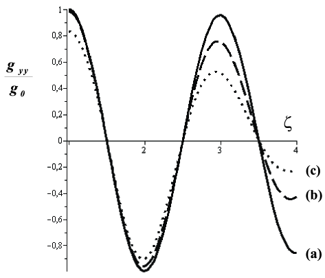
Figure 3: Attenuation of spin current oscillations due to finite widths of the ring and leads, at a zero magnetic field. $g_{yy}$ is the $y$-component of the spin conductance along the $y$-axis, see (3) in the text. $g_{0}$ is the transmitted flux of electrons per unit energy interval, per one spin projection of the incident electrons. The variable $\zeta$ is expressed in terms of the spin-orbit length $L_{SO}$ as $\zeta=\sqrt{1+4(a/L_{SO})^{2}}$. Three curves correspond to parameter sets
(a) $a=1\>\mu\,,\,\,d=150\>nm\,\,,\,\,W=150\>nm\,\,,\,\,q=1/2\,$;
(b) $a=1,5\>\mu\,,\,\,d=300\>nm\,\,,\,\,W=100\>nm\,\,,\,\,q=1/5\,$;
(c) $a=1,5\>\mu\,,\,\,d=300\>nm\,\,,\,\,W=30\>nm\,\,,\,\,q=1/5\,$.

The denominator in (64) gives rise to a set of peaks with maxima at $\zeta=\zeta_{m}\equiv m$, where $m$ is integer. It is easily seen that for $T_{1}^{-1}\gg\tau^{-1}+\tau_{\perp}^{-1}$ the peak’s broadening $\Delta_{g}\ll 1$. Due to this inequality Eq. (64) can be written in the vicinity of peaks in a more simple form:

$$\langle g_{yy}\rangle=(-1)^{m+1}g_{0}\frac{\frac{T_{1}}{2\pi^{2}}\frac{1}{\tau}}{\left(\Delta\zeta\right)^{2}+\frac{T_{1}}{2\pi^{2}}\left(\frac{1}{\tau}+\frac{1}{\tau_{\perp}}\right)}\,,$$ (65)

where $\Delta\zeta=\zeta-\zeta_{m}$. From Eq. (65) $\Delta_{g}$ is expressed as

$$\Delta_{g}=\sqrt{\frac{2T_{1}}{\pi^{2}}\left(\frac{1}{\tau}+\frac{1}{\tau_{\perp}}\right)}\,.$$ (66)

Note, that as follows from (124), $\tau_{\perp}$ depends on $\zeta$. Hence, $\Delta_{g}$ depends on the resonance $\zeta_{m}$ position.

In the case of a long particle lifetime $\tau\gg\tau_{\perp}$ one obtains from Eq. (124)

$$\Delta_{g}=\gamma_{m}^{2}\frac{d}{a}\sqrt{\frac{8(1+\zeta^{2}_{m})}{3\zeta^{2}_{m}}}\,.$$ (67)

For example, the broadening of the third peak ($\zeta_{m}=3,\gamma_{m}=\sqrt{2}$) is $\Delta_{g}\simeq 3.4d/a$. It is a quite noticeable value for a typical ratio $d/a\sim 0.1$

So, the first obvious effect of the finite width is the broadening of the spin current oscillation peaks. The physical origin of this effect is the increased relaxation rate of the spin polarization. This relaxation is caused by incoherent superposition of polarizations coming from the trajectories encircling slightly different areas in a ring of finite width. The situation is elucidated in Fig. 4. This picture shows that the finite width results in adding random loops breaking the coherency of the trajectories.

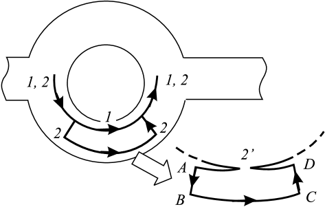
Figure 4: A schematic picture explaining the effect of finite width. Since the element of the trajectory passed forward and backward does not give a contribution to the evolution operator,one can replace the trajectory $2$ by $2^{\prime}$. After that it is obvious that the difference between $1$ and $2$ is that the latter contains the loop $ABCD$ passed counterclockwise.

In addition to the broadening, the increased relaxation rate leads, evidently, to a reduction of the peak intensity. This is explicitly given by

$$\left|\left<g_{yy}\right>_{\zeta=\zeta_{m}}\right|=\frac{g_{0}}{1+\frac{\tau}{\tau_{\perp}}}\,$$ (68)

which is the spin current magnitude exactly at maxima (minima). From Appendix C the ratio of times in the denominator of (68) can be expressed as

$$\frac{\tau}{\tau_{\perp}}\simeq\frac{1}{6\pi q}\frac{\gamma^{4}(1+\zeta^{2})}{\zeta^{2}}\frac{a}{W}\left(\frac{d}{a}\right)^{4}\ln^{2}\frac{2a}{d}\,.$$ (69)

This expression shows that the finite width effect is suppressed fast with smaller $d/a$.

Now let us focus on magnetic field effects. The first effect is that the components $\langle g_{yz}\rangle$, $\langle g_{zy}\rangle$, $\langle g_{xy}\rangle$, $\langle g_{yx}\rangle$ of the spin conductance are no longer zero. One can verify from Eqs. (14), (11) and (8) that they appear because the reflection symmetry with respect to the $XOZ$-plane is broken by the magnetic field. The physical meaning of such nondiagonal components can be explained in terms of the effective polarization $\bm{P}_{eff}(\bm{e}_{j})$ on the exit from the ring, see Eq. (16). For example, nonzero $\langle g_{zy}\rangle$ and $\langle g_{xy}\rangle$ are associated with a rotation of $\bm{P}_{eff}(\bm{e}_{y})$ with respect to the polarization $\bm{e}_{y}$ of the left reservoir. It is convenient to consider a projection of $\bm{P}_{eff}(\bm{e}_{y})$ onto $YOZ$-plane. Then, the rotation angle $\phi_{P}$ of this projection can be calculated from Eqs. (62) and (63). For the $m$-th peak this angle is given by

$$\tan\phi_{P}=-\frac{2\gamma}{\zeta_{m}}\frac{\frac{\omega_{H}}{\zeta_{m}}}{\frac{1}{\tau}+\frac{1}{\tau_{\perp}}}\,.$$ (70)

The nonzero $\langle g_{yz}\rangle$, $\langle g_{yx}\rangle$ components can be interpreted in a similar way. We note, that due to the linear dependence on $\omega_{H}$, the sign of $\phi_{P}$ changes together with the magnetic field.

Another effect of the magnetic field is a reduction of the spin current. Let us consider a trajectory which contains a narrow loop, see Fig. 5.

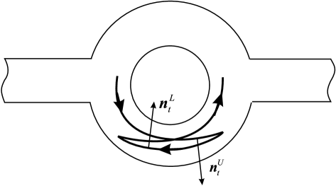
Figure 5: Narrow loops of the trajectory which break the coherence of the trajectories in the presence of the magnetic field.

If the magnetic field is ignored and only the SOI effect is taken into account, after passing the loop the polarization $\bm{P}$ does not change. That is because on the upper and the lower parts of the loop $\bm{P}$ rotates in opposite directions, according to opposite directions $\bm{n}_{t}^{U}$ and $\bm{n}_{t}^{L}$ of the SOI fields, see Eq. (8). A magnetic field, however, causes rotations of $\bm{P}$ in the same directions. Hence, evolutions of $\bm{P}$ along trajectories with and without the loop becomes different. This introduces an additional decoherence leading to the spin current reduction and broadening of its oscillation peaks. Using (62) and (63) one can derive the following expression for the magnitude of the effective polarization exactly at maxima (minima)

$$\left.P_{eff}(\bm{e}_{y})\right|_{\zeta=\zeta_{m}}$$

$$=g_{0}^{-1}\sqrt{\left|\langle g_{yy}\rangle_{\zeta=\zeta_{m}}\right|^{2}+\left|\langle g_{zy}\rangle_{\zeta=\zeta_{m}}\right|^{2}+\left|\langle g_{xy}\rangle_{\zeta=\zeta_{m}}\right|^{2}}$$

$$\simeq\left[1+\left(\frac{\omega_{H}\tau}{\zeta_{m}}\right)^{2}\right]^{-1/2}\,,$$ (71)

provided that the ring is narrow enough, $\tau/\tau_{\perp}\ll\omega_{H}\tau/\zeta_{m}$.

Let us consider a dependence of the spin conductance on $\zeta$ in the presence of the magnetic field. In the the vicinity of the $m$-th peak, instead of (65) wehave

$$\langle g_{yy}\rangle=g_{0}(-1)^{m+1}\frac{\frac{1}{\tau}\left[\frac{1}{\tau}+\frac{1}{\tau_{\perp}}+\frac{2\pi^{2}}{T_{1}}(\Delta\zeta)^{2}\right]}{\left[\frac{1}{\tau}+\frac{1}{\tau_{\perp}}+\frac{2\pi^{2}}{T_{1}}(\Delta\zeta)^{2}\right]^{2}+\left(\frac{\omega_{H}}{\zeta_{m}}\right)^{2}}\,.$$ (72)

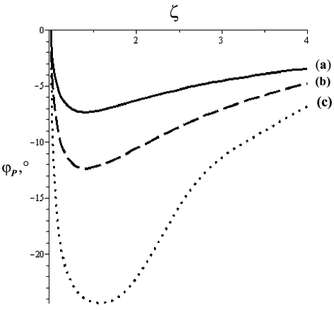
Figure 6: Rotation of the effective polarization vector $\bm{P}_{eff}(\bm{e}_{y})$ on the exit from the ring in the presence of the magnetic field. $\phi_{P}$ is the angle between the initial polarization $\bm{e}_{y}$ of the electrons in the left reservoir and projection of $\bm{P}_{eff}(\bm{e}_{y})$ onto the $YOZ$ plane. The magnetic field strength is 100G. Curves (a), (b) and (c) correspond to the same parameter sets as in Fig. 3.

As can be seen from this equation, the relaxation mechanism associated with the magnetic field gives rise to an additional broadening of spin current peaks. Their width can be evaluated from Eq. (72) as

$$\Delta_{g}=\sqrt{\frac{2T_{1}}{\pi^{2}}}\left[\left(\frac{1}{\tau}+\frac{1}{\tau_{\perp}}\right)^{2}+\left(\frac{\omega_{H}}{\zeta_{m}}\right)^{2}\right]^{1/4}.$$ (73)

The discussed above effects are determined by characteristic times $\tau$, $T_{1}$ and $\tau_{\perp}$. These times have been evaluated in Appendix C using a simple model of scattering from a bumpy ring boundary. Fig. 3 and Fig. 6 demonstrate the effects of the ring width and magnetic field on behavior of the spin conductance as a function of $\zeta=\sqrt{1+4(a/L_{so})^{2}}$. We took $k_{F}\simeq 2.5\times 10^{6}\>cm^{-1}$ and $L_{so}$ varying in a wide range. In InAs based quantum wells SOI can be quite strong with $L_{so}$ being as small, as $\sim 100$ nmGrundler ; Nitta . For $a=1\mu$ this gives $\zeta=20$. Curve (a) in these figures corresponds to the escape time much shorter than $T_{1}$ and $\tau_{\perp}$. The winding number is not large and AC resonances are broad. There are no noticeable effects associated with the finite ring width. Also, the magnetic field effect is relatively weak. The width effects are seen on the curve (b), in Fig. 3. A reduction of the oscillation amplitude seen in the figure is in a qualitative agreement with Eq. (68), although for considered parameters this equation can not be fully applied, because the winding number is not large enough. The winding number is larger for the third set of parameters, (c). The finite width effect becomes stronger , leading to a faster decreasing of the oscillation amplitude. Also stronger is the magnetic field effect on polarization rotation in the $xy$-plane (see Fig. 6). Strictly speaking, our semiclassical theory can not be applied to this case, because the number of propagating channels in leads is not large. We, nevertheless show this result in order to demonstrate a trend: for reasonable ring sizes the regime of large windings with sharp AC resonances can be achieved only at small lead widths, or by means of barriers between leads and the ring, resulting in the long $\tau$.

We note that the magnetic field effect on polarization rotation is rather noticeable even at relatively weak 100 Gauss magnetic fields, as can be seen at Fig. 6. For example, for $\zeta=1.6$ and parameters (c), the rotation angle can be as large as $24^{\circ}$.

Appendix A Landauer formula for the spin current

Since the spin current density is an additive one-particle dynamical observable, its average value at the point ${\bf R}$ and $t=0$ is given by

$$\langle J_{lj}({\bf R},t=0)\rangle={\rm Tr}\left\{\hat{f}_{1}(t=0)\hat{J}_{1}^{lj}({\bf R})\right\}$$ (74)

Here the one-particle distribution function $\hat{f}_{1}$ describes the open system consisting of the leads and the ring. The one-particle operator

$$\hat{J}_{1}^{lj}({\bf R})=\frac{\hat{v}_{l}\hat{{\cal P}}_{j}({\bf R})+\hat{{\cal P}}_{j}({\bf R})\hat{v}_{l}}{2}$$ (75)

represents $l$-th component of the current density with spins polarized along $j$-th coordinate axis. $\hat{v}_{l}$ is $l$-th component of the electron velocity operator. Since we calculate the spin current in the asymptotic region of the right lead, where the magnetic field and SOI are zero, the operator $\hat{v}_{i}$ may be written simply as $\hat{p}_{i}/m^{*}$, where $\hat{\mathbf{p}}$ is the electron momentum operator. The polarization density $\hat{{\cal P}}_{j}({\bf R})$ is defined by

$$\hat{{\cal P}}_{j}({\bf R})=\hat{\rho}_{\bf R}\,\hat{\sigma_{j}}\,,$$ (76)

where $\hat{\rho}_{\bf R}$ is the density operator. In the the coordinate representation the latter is given by

$$\hat{\rho}_{\bf R}=\delta({\bf r}-{\bf R})\,.$$ (77)

It should be noted that Eq. (74) represents a polarization current density, rather then the spin current density, which is twice smaller. For convenience we will use, however, the latter name.

For noninteracting electrons the evolution of the distribution function is described by the equation

$$i\hbar\frac{\partial\hat{f}_{1}}{\partial t}=[H,\hat{f}_{1}]\,$$ (78)

where $H$ is the one-particle Hamiltonian for the system ”leads+ring”. A formal solution of Eq.(78) may be written in the form

$$\hat{f}_{1}(t)=\hat{U}(t,t_{0})\hat{f}_{1}(t_{0})\hat{U}^{+}(t,t_{0})\,,$$ (79)

$$\hat{U}(t,t_{0})=e^{-i\hat{H}(t-t_{0})/\hbar}\,.$$ (80)

Further, we take into account that the system under consideration has an asymptotic region where an electron is effectively decoupled from the ring. In this case the methods of the scattering theory may be applied directly, without adiabatic switching off the scattering potential at $t=\pm\infty$. First, let us write down $\hat{f}_{1}(0)$ in the form

$$\hat{f}_{1}(0)=\lim_{T\rightarrow+\infty}\hat{U}(0,-T)\hat{U}_{0}^{+}(0,-T)\hat{U}_{0}(0,-T)\\ \times\hat{f}_{1}(-T)\hat{U}_{0}^{+}(0,-T)\hat{U}_{0}(0,-T)\hat{U}^{+}(0,-T)\,,$$ (81)

where the unperturbed evolution operator $\hat{U}_{0}$ is obtained from (80) by replacing $\hat{H}$ with the ”unperturbed” Hamiltonian $\hat{H}_{0}$. The latter is obtained by removing the ring and elongating the leads to meet each other. In Eq. (81) one easily recognizes the familiar Möller operator $\Omega_{+}$ of the scattering theory Taylor ,

$$\Omega_{+}=\lim_{T\rightarrow+\infty}\hat{U}(0,-T)\hat{U}_{0}^{+}(0,-T)\,.$$ (82)

This operator maps the wave function $\left|\psi_{in}\right>$ describing a particle state at $t=0$ in the absence of the ring onto the actual state $\left|\psi(t=0)\right>$ :

$$\left|\psi(t=0)\right>=\Omega_{+}\left|\psi_{in}\right>\,.$$ (83)

From (82) and (81) we obtain

$$\hat{f}_{1}(0)=\Omega_{+}\hat{f}_{1}^{in}\left(\Omega_{+}\right)^{+}\,,$$ (84)

where, by analogy with $\left|\psi_{in}\right>$, the function

$$\hat{f}_{1}^{in}=\lim_{T\rightarrow+\infty}\hat{U}_{0}(0,-T)\hat{f}_{1}(-T)\hat{U}_{0}^{+}(0,-T)$$ (85)

can be interpreted as a distribution function of the system at $t=0$ in the absence of the ring. The trace in (74) can now be rewritten as

$$\langle J_{lj}({\bf R},t=0)\rangle=\sum_{i_{1},i_{2}}\left<i_{1}\right|\hat{f}_{1}^{in}\left|i_{2}\right>\\ \times\left<i_{2}\right|\left(\Omega_{+}\right)^{+}\hat{J}_{1}^{lj}\left({\bf R}\right)\Omega_{+}\left|i_{1}\right>\,.$$ (86)

Since the unperturbed problem does not involve SO interaction, a convenient choice of the basis vectors $\left|i\right>$ in (86) is

$$\left|i\right>=\left|b\right>\otimes\left|\alpha\right>\,,$$ (87)

where the eigenvector $\left|b\right>$ corresponding to the unperturbed Hamiltonian describes the electron orbital motion and $\left|\alpha\right>$ is the eigenvector of $\hat{\sigma}_{z}$ corresponding to its eigenvalue $\alpha$. Further, the slab geometry of the unperturbed problem suggests that $\left|b\right>$ is taken in the form

$$\left|b\right>=\left|k\right>\otimes\left|p\right>\otimes\left|m\right>\,,$$ (88)

with the eigenvectors $\left|k\right>,\left|p\right>,\left|m\right>$ describing a particle motion along $OX,OY,OZ$ axes in the absence of the ring. Hence, the corresponding wave functions are

$$w_{k}(x)=\left<x\right|\left.k\right>=\frac{1}{\sqrt{L}}e^{ikx}\,,$$ (89)

$$v_{p}(y)=\left<y\right|\left.p\right>=\sqrt{\frac{2}{L_{y}}}\,sin{(k_{y}y)}$$ (90)

$$k_{y}=\frac{\pi}{L_{y}}p\,,\,\,(p=1,2,...)$$ (91)

and similarly for the wave function $u_{m}(z),\,m=1,2,...$, in z-direction. We took periodic boundary conditions in x-direction, where $L$ is the total length of the system. At the slab interfaces the wave functions $v_{p}(y)$ and $u_{m}(z)$ satisfy the hard wall boundary conditions.

Unit vectors parallel to polarizations of the left and right reservoirs will be denoted as $\bm{\nu}^{L}$ and $\bm{\nu}^{R}$, respectively. Accordingly, we define the operators $\hat{\sigma}_{\nu^{L,R}}\equiv\sum_{i}\hat{\sigma}_{i}\nu^{L,R}_{i}$ with eigenvectors $\left|\nu^{L,R}\sigma\right>$ corresponding to polarization projections $\sigma=\uparrow,\downarrow$ onto $\bm{\nu}^{L}$ and $\bm{\nu}^{R}$. Since particles with different spins are distributed in reservoirs according to their respective Fermi distributions, the magnitudes of the reservoirs polarizations are determined by the differences $\delta\mu_{L,R}=\mu_{\nu^{L,R}\uparrow}-\mu_{\nu^{L,R}\downarrow}$ of chemical potentials of spin up and spin down (relative to $\bm{\nu}^{L,R}$) electron gas components. Therefore, assuming that the unperturbed distributions of particles moving to the right ($k>0$) and to the left ($k<0$) are given by the Fermi distributions in the left and right reservoirs, respectively, we can write

$$\hat{f}_{1}^{in}=\sum_{b,\sigma}\Theta\left(k\right)n_{b,\nu^{L}\sigma}\left(\left|b\right>\left<b\right|\right)\otimes\left(\left|\nu^{L}\sigma\right>\left<\nu^{L}\sigma\right|\right)\\ +\sum_{b,\sigma}\Theta\left(-k\right)n_{b,\nu^{R}\sigma}\left(\left|b\right>\left<b\right|\right)\otimes\left(\left|\nu^{R}\sigma\right>\left<\nu^{R}\sigma\right|\right)\,,$$ (92)

where $\Theta(\cdot)$ is the Heaviside step function and

$$n_{b,\nu^{L}\sigma}=\Theta\left(\mu_{\nu^{L}\sigma}-E\right)\,,\,\,n_{b,\nu^{R}\sigma}=\Theta\left(\mu_{\nu^{R}\sigma}-E\right)$$ (93)

are the Fermi distributions in the left and right reservoirs for particles with the energy $E$. Note, that Eq. (92) was written under the assumption that contacts between reservoirs and leads are adiabatic (no scattering from the contacts).

We assume for the average chemical potentials $\mu_{L}=\mu_{R}$, where $\mu_{L/R}=(\mu_{\nu^{L/R}\uparrow}+\mu_{\nu^{L/R}\downarrow})/2$. So, the chemical potentials of unpolarized reservoirs coincide. Denoting them $\mu_{U}$ we write the distribution function corresponding to the unpolarized reservoirs in the form

$$\hat{f}_{1}^{U}=\sum_{b}n^{U}_{b}\left(\left|b\right>\left<b\right|\right)\otimes\sigma_{0},$$ (94)

where $n^{U}_{b}=\Theta(\mu_{U}-E)$. Evidently, $\hat{f}_{1}^{U}$ does not give any contribution to $\langle J_{lj}({\bf R},t=0)\rangle$. Therefore, it is convenient to subtract this function from $\hat{f}^{in}_{1}$:

$$\hat{f}_{1}^{in}=\hat{f}_{1}^{U}+\delta\hat{f}_{1}^{L}+\delta\hat{f}_{1}^{R}$$ (95)

$$\delta\hat{f}_{1}^{L}=\sum_{b,\sigma}\Theta\left(k\right)\delta n_{b,\nu^{L}\sigma}\left(\left|b\right>\left<b\right|\right)\otimes\left(\left|\nu^{L}\sigma\right>\left<\nu\sigma^{L}\right|\right)$$ (96)

$$\delta\hat{f}_{1}^{R}=\sum_{b,\sigma}\Theta\left(-k\right)\delta n_{b,\nu^{R}\sigma}\left(\left|b\right>\left<b\right|\right)\otimes\left(\left|\nu^{R}\sigma\right>\left<\nu^{R}\sigma\right|\right)$$ (97)

$$\delta n_{b,\nu^{L,R}\sigma}=n_{b,\nu^{L,R}\sigma}-n_{b}^{U}$$ (98)

Denoting corresponding contributions of $\delta\hat{f}_{1}^{L}$ and $\delta\hat{f}_{1}^{R}$ to the spin current as $\langle J_{lj}({\bf R},t=0)\rangle_{L}$ and $\langle J_{lj}({\bf R},t=0)\rangle_{R}$, we arrive at

$$\langle J_{lj}({\bf R},t=0)\rangle=\langle J_{lj}({\bf R},t=0)\rangle_{L}+\langle J_{lj}({\bf R},t=0)\rangle_{R}\,.$$ (99)

The projectors $\left|\nu^{L}\sigma\right>\left<\nu^{L}\sigma\right|$ and $\left|\nu^{R}\sigma\right>\left<\nu^{R}\sigma\right|$ in (96) and (97) can be expressed in terms of the Pauli matrices $\hat{\sigma}_{\nu^{L,R}}$ and the unit matrix $\hat{\sigma}_{0}$ using easily verified relations

$$\hat{\sigma}_{\nu}=\left(\left|\nu\uparrow\right>\left<\nu\uparrow\right|\right)-\left(\left|\nu\downarrow\right>\left<\nu\downarrow\right|\right)$$

$$\hat{\sigma}_{0}=\left(\left|\nu\uparrow\right>\left<\nu\uparrow\right|\right)+\left(\left|\nu\downarrow\right>\left<\nu\downarrow\right|\right)$$

Straightforward calculations then give

$$\langle J_{lj}({\bf R},t=0)\rangle_{L,R}=\sum_{\begin{subarray}{c}b,\alpha_{1},\alpha_{2}\\ \mu_{U}-\frac{\delta\mu_{L,R}}{2}<E<\mu_{U}+\frac{\delta\mu_{L,R}}{2}\end{subarray}}\Theta(\pm k)\frac{\sigma_{\nu^{L,R}}^{\alpha_{1}\alpha_{2}}}{2}\\ \times\left<b\alpha_{2}\right|\left(\Omega_{+}\right)^{+}\hat{J}_{1}^{lj}\left({\bf R}\right)\Omega_{+}\left|b\alpha_{1}\right>\,,$$ (100)

where $\left|b\alpha_{1,2}\right>\equiv\left|b\right>\otimes\left|\alpha_{1,2}\right>$, and upper (lower) sign in the argument of $\Theta$-function corresponds to the index ”L” (”R”). The leads are assumed to be thin enough in z-direction, so that only the levels $\left|b\right>=\left|kpm\right>$ with $m=1$ are occupied and contribute to the sum in Eq. (100). For simplicity, we denote

$$\left|kp\right>=\left|kp,m=1\right>\,,$$ (101)

It is convenient to change in (100) the summation over $k$ by integration over $E$. To do this, we introduce the vectors

$$\left|Ep\right>^{(\pm)}=\sqrt{\nu_{p}(E)}\left|kp\right>$$ (102)

$$\nu_{p}(E)=\frac{L}{2\pi\hbar\,v_{p}(E)}\,,$$

where $\pm$ signs relate to $k>0$ and $k<0$. $\nu_{p}(E)$ is the one-dimensional density of states in the $p$-th channel, and $v_{p}(E)=\sqrt{2(E-E_{p})/m^{*}}$ is the electron velocity in $p$-th channel characterized by the kinetic energy in $y$-direction $E_{p}$. Using definitions (102) one can write

$$\sum_{\begin{subarray}{c}b\\ \mu_{U}-\frac{\delta\mu_{L,R}}{2}<E<\mu_{U}+\frac{\delta\mu_{L,R}}{2}\end{subarray}}\Theta(\pm k)\left<b\right|\cdot\left|b\right>\\ =\sum_{p}\int_{\mu_{U}-\frac{\delta\mu_{L,R}}{2}}^{\mu_{U}+\frac{\delta\mu_{L,R}}{2}}dE\hskip 5.69054pt{{}^{(\pm)}}\left<Ep\right|\cdot\left|Ep\right>^{(\pm)}\,,$$ (103)

Further, in the limit $L\rightarrow+\infty$ considering $E$ as a continuous variable one gets the normalization condition

$${{}^{(\pm)}}\left<E^{\prime}p^{\prime}\right|\left.Ep\right>^{(\pm)}=\delta_{p^{\prime}p}\delta(E^{\prime}-E)\,.$$ (104)

Using this condition and substituting (103) into Eq. (100) we find

$$\langle J_{lj}({\bf R},t=0)\rangle_{L,R}=\sum_{p,\alpha_{1},\alpha_{2}}\int_{\mu_{U}-\frac{\delta\mu_{L,R}}{2}}^{\mu_{U}+\frac{\delta\mu_{L,R}}{2}}dE\,\frac{\sigma_{\nu^{L,R}}^{\alpha_{1}\alpha_{2}}}{2}\\ \times{{}^{(\pm)}}\left<Ep\,\alpha_{2}\right|\left(\Omega_{+}\right)^{+}\hat{J}_{1}^{lj}\left({\bf R}\right)\Omega_{+}\left|Ep\,\alpha_{1}\right>^{(\pm)}\,,$$ (105)

($\left|Ep\,\alpha_{1,2}\right>^{(\pm)}\equiv\left|Ep\right>^{(\pm)}\otimes\left|\alpha_{1,2}\right>$). In its turn, the total spin current through the cross section of the right lead is given by

$$\langle J_{j}(X,t=0)\rangle_{L,R}=\int dYdZ\langle J_{xj}({\bf R},t=0)\rangle_{L,R}\,.$$

Using Eq. (105) we obtain

$$\langle J_{j}(X,t=0)\rangle_{L,R}\\ =\sum_{p,\alpha_{1},\alpha_{2}}\int_{\mu_{U}-\frac{\delta\mu_{L,R}}{2}}^{\mu_{U}+\frac{\delta\mu_{L,R}}{2}}dE\,\frac{\sigma_{\nu^{L,R}}^{\alpha_{1}\alpha_{2}}}{2}\int dYdZ\\ \times{{}^{(\pm)}}\left<Ep\,\alpha_{2},+\right|\hat{J}_{1}^{xj}\left({\bf R}\right)\left|Ep\,\alpha_{1},+\right>^{(\pm)}\,,$$ (106)

where

$$\left|Ep\,\alpha_{s},+\right>^{(\pm)}=\Omega_{+}\left|Ep\,\alpha_{s}\right>^{(\pm)}\,,\,\,s=1,2\,.$$

The vectors $\left|Ep\,\alpha_{s},+\right>^{(\pm)}$ are known Taylor as the scattering states associated with the ”in” asymptotes (”incident waves”) $\left|Ep\,\alpha_{s}\right>^{(\pm)}$. Since the point $\bf R$ in the r.h.s of (106) is located in the asymptotic region of the right lead, only the asymptotic behavior of the wave functions $\phi^{(\pm)}_{Ep\,\alpha_{2},+}({\bf R}\alpha)\equiv\left<{\bf R}\alpha\right|\left.Ep\,\alpha_{2},+\right>^{(\pm)}$ and $\phi^{(\pm)}_{Ep\,\alpha_{1},+}({\bf R}\beta)$ affects the calculation of the matrix elements in (106). Thus, we may write $\phi^{(+)}_{Ep\,\alpha_{2},+}({\bf R}\alpha)$ and $\phi^{(+)}_{Ep\,\alpha_{1},+}({\bf R}\alpha)$ as the sum of transmitted waves while $\phi^{(-)}_{Ep\,\alpha_{2},+}({\bf R}\alpha)$ and $\phi^{(-)}_{Ep\,\alpha_{1},+}({\bf R}\alpha)$ as the sum of incident and reflected waves,

$$\phi^{(+)}_{Ep\,\alpha_{2},+}({\bf R}\alpha) =\sum_{p^{\prime\prime}\alpha^{\prime\prime}}t_{p^{\prime\prime}p}^{\alpha^{\prime\prime}\alpha_{2}}(E)\phi^{(+)}_{Ep^{\prime\prime}\alpha^{\prime\prime}}({\bf R}\alpha)$$ (107a)

$$\phi^{(-)}_{Ep\,\alpha_{2},+}({\bf R}\alpha) =\phi^{(-)}_{Ep\,\alpha_{2}}({\bf R}\alpha)$$

$$+\sum_{p^{\prime\prime}\alpha^{\prime\prime}}r_{p^{\prime\prime}p}^{\alpha^{\prime\prime}\alpha_{2}}(E)\phi^{(+)}_{Ep^{\prime\prime}\alpha^{\prime\prime}}({\bf R}\alpha),$$ (107b)

where $t_{p^{\prime\prime}p}^{\alpha^{\prime\prime}\alpha_{2}}(E)$ and $r_{p^{\prime\prime}p}^{\alpha^{\prime\prime}\alpha_{2}}(E)$ denote transmission and reflection amplitudes, respectively. According to (102) and (101)

$$\phi^{(\pm)}_{Ep^{\prime\prime}\,\alpha^{\prime\prime}}({\bf R}\alpha)=\xi^{(\pm)}_{p^{\prime\prime}E}(X)u_{p^{\prime\prime}}(Y)v_{1}(Z)\chi_{\alpha^{\prime\prime}}(\alpha)\,,$$ (108)

where

$$\xi^{(\pm)}_{p^{\prime\prime}E}(X)=\sqrt{\nu_{p^{\prime\prime}}(E)}w_{\pm k}(X)=\frac{1}{\sqrt{2\pi\hbar v_{p^{\prime\prime}}(E)}}\,e^{\pm ikX},$$ (109)

and $\chi_{\alpha^{\prime\prime}}(\alpha)=\left<\alpha\right|\left.\alpha^{\prime\prime}\right>$. $k$ in (109) is the positive solution of the equation $E-E_{p"}=\hbar^{2}k^{2}/2m^{*}$. Note, that due to our choice of the prefactor in (102), the functions $\xi_{p^{\prime\prime}E}(X)$ ”carry” the same flux $(2\pi\hbar)^{-1}$, independent on the channel number $p^{\prime\prime}$. As a result, the transmission and reflection amplitudes satisfy the flux conservation law

$$\sum_{p"\alpha"}\left\{\left|t_{p"p}^{\alpha"\alpha_{2}}\right|^{2}+\left|r_{p"p}^{\alpha"\alpha_{2}}\right|^{2}\right\}=1$$

Using Eq. (75) and Eqs. (107) – (108), we transform Eq. (106) into

$$\begin{split}&\langle J_{j}\left(X,t=0\right)\rangle_{L}\\ &=\frac{\delta\mu_{L}}{2\pi\hbar}\sum_{p,p^{\prime}}\frac{1}{2}\,{\rm Tr}\left\{\hat{t}_{p^{\prime}p}^{+}(\mu_{U})\,\hat{\sigma}_{j}\,\hat{t}_{p^{\prime}p}(\mu_{U})\,\hat{\sigma}_{\nu^{L}}\,\right\}\end{split}$$ (110a)

$$\begin{split}\langle J_{j}\left(X,t=0\right)\rangle_{R}\quad&\\ =\frac{\delta\mu_{R}}{2\pi\hbar}\left[\vphantom{\frac{1}{2}}\right.\sum_{p,p^{\prime}}\frac{1}{2}&\,{\rm Tr}\left\{\hat{r}_{p^{\prime}p}^{+}(\mu_{U})\,\hat{\sigma}_{j}\,\hat{r}_{p^{\prime}p}(\mu_{U})\,\hat{\sigma}_{\nu^{R}}\,\right\}\\ &-\left.N_{m}(\mu_{U})\frac{1}{2}\,{\rm Tr}\left\{\hat{\sigma}_{\nu^{R}}\hat{\sigma}_{j}\right\}\right]\end{split}$$ (110b)

where $\hat{t}_{p^{\prime}p}(\mu_{U})$ is the $2\times 2$ matrix composed of the transmission amplitudes $t_{p^{\prime}p}^{\uparrow\uparrow}(\mu_{U})$,$\,t_{p^{\prime}p}^{\uparrow\downarrow}(\mu_{U})\,$, $t_{p^{\prime}p}^{\downarrow\uparrow}(\mu_{U})\,$, $t_{p^{\prime}p}^{\downarrow\downarrow}(\mu_{U})\,$. The matrix $\hat{r}_{p^{\prime}p}(\mu_{U})$ is composed in a similar way. Taking into account that $\hat{\sigma}_{\nu}=\hat{\vec{\sigma}}\cdot\vec{\nu}$ $=\hat{\sigma}_{i}\nu_{i}$ and denoting

$$g^{L}_{ji}=\frac{1}{2\pi\hbar}\sum_{pp^{\prime}}\frac{1}{2}{\rm Tr}\left\{\hat{t}_{p^{\prime}p}^{+}(\mu_{U})\,\hat{\sigma}_{j}\,\hat{t}_{p^{\prime}p}(\mu_{U})\,\hat{\sigma}_{i}\right\}$$ (111a)

$$\begin{split}g^{R}_{ji}=\frac{1}{2\pi\hbar}\left[\vphantom{\frac{1}{2}}\right.\sum_{pp^{\prime}}\frac{1}{2}{\rm Tr}\left\{\hat{r}_{p^{\prime}p}^{+}(\mu_{U})\,\hat{\sigma}_{\hskip 2.84526ptj}\,\hat{r}_{p^{\prime}p}(\mu_{U})\,\hat{\sigma}_{\hskip 2.84526pti}\right\}&\\ -N_{m}(\mu_{U})\delta_{ij}&\left.\vphantom{\frac{1}{2}}\right]\end{split}$$ (111b)

we rewrite (110) in the form

$$\langle J_{j}\left(X,t=0\right)\rangle_{L,R}=\sum_{i}\;g^{L,R}_{ji}\;\nu^{L,R}_{i}\;\delta\mu_{L,R}\,.$$ (112)

We shall call the $3\times 3$ matrices $g^{L}$ and $g^{R}$ as spin conductances. They determine the response of the spin current to the polarization of the left and right reservoirs, respectively. For example, if the left reservoir is polarized along the $s$-th axis, $\bm{\nu}^{L}=\bm{e}_{s}$ ($\bm{e}_{s}$ is the $s$-th coordinate ort), and the right reservoir is unpolarized, then according to (99) and (112) $\langle J_{j}\left(X,t=0\right)\rangle=g^{L}_{js}\delta\mu_{L}$ and $g^{L}_{js}$ proves be the proportionality coefficient between $\delta\mu_{L}$ and $j$-th component of the spin current.

It is convenient to express the quantities $\nu^{L}_{i}\delta\mu_{L}$ and $\nu^{R}_{i}\delta\mu_{R}$ in Eq. (112) in terms of 2D spin polarization densities $\langle{\cal P}_{i}(XY)\rangle_{L}$ and $\langle{\cal P}_{i}(XY)\rangle_{R}$ corresponding to chemical potentials of the left and right reservoirs. At small $\delta\mu_{L}$ and $\delta\mu_{R}\ll E_{F}$ we have

$$\langle{\cal P}_{i}(XY)\rangle_{L/R}=N_{F}\nu^{L/R}_{i}\delta\mu_{L/R}\,,$$ (113)

where $N_{F}=2\pi m^{*}/h^{2}$ is the 2D electron state density. Substituting this expression into Eq. (112) we rewrite the latter in the form

$$\langle J_{j}\left(X,t=0\right)\rangle_{L,R}=\frac{2\pi\hbar^{2}}{m^{*}}\sum_{i}g^{L,R}_{ji}\langle{\cal P}_{i}(XY)\rangle_{L,R}\,.$$ (114)

Combining (99), (112), and (114) we obtain finally

$$\langle J_{j}\left(X,t=0\right)\rangle=\langle J_{j}\left(X,t=0\right)\rangle_{L}+\langle J_{j}\left(X,t=0\right)\rangle_{R}\\ =\sum_{i}\;g^{L}_{ji}\;\nu^{L}_{i}\;\delta\mu_{L}+\sum_{i}\;g^{R}_{ji}\;\nu^{R}_{i}\;\delta\mu_{R}\\ =\frac{2\pi\hbar^{2}}{m^{*}}\left\{\sum_{i}g^{L}_{ji}\langle{\cal P}_{i}(XY)\rangle_{L}+\sum_{i}g^{R}_{ji}\langle{\cal P}_{i}(XY)\rangle_{R}\right\}\,,$$ (115)

This expression gives the spin current in the right lead in terms of the left and right reservoir polarizations.

Comparing our expression (111) for the spin conductance with the Landauer formula we see that they are different in the way that our spin conductance is written in terms of both transmission and reflection coefficients. This difference is of principal character since due to nonconservation of spin current we can not express the contribution $\langle J_{j}\left(X,t=0\right)\rangle_{R}$ (containing the reflection coefficients) via the spin current in the left lead transmitted from the right.

Appendix B Evolution of polarization along $s$-th trajectory

If we define the polarization of an electron as

$${\bm{P}}={\rm Tr}\left\{\hat{\rho}\,\hat{\bm{\sigma}}\right\}\,,$$ (116)

then, according to Ref. Gottfr, the density matrix describing its spin state may be represented in the form

$$\hat{\rho}=\frac{1}{2}\left\{\hat{\sigma_{0}}+{\bm{P}}\cdot\hat{\bm{\sigma}}\right\}\,,$$ (117)

where $\hat{\sigma_{0}}$ is the $2\times 2$ unit matrix. After passing $s$-th trajectory, the spin density matrix is transformed into

$$\hat{\rho}^{\prime}=\hat{S}_{s}\hat{\rho}\hat{S}_{s}^{+}\,,$$ (118)

where $\hat{S}_{s}$ is the spin evolution operator given by Eq. (8). Substituting (117) into (118) and then (118) into (116) we obtain the polarization of the electron at the end of the $s$-th trajectory

$${\bm{P}^{\prime}}=\frac{1}{2}{\rm Tr}\left\{\hat{S}_{s}\left({\bm{P}}\cdot\hat{\bm{\sigma}}\right)\hat{S}_{s}^{+}\hat{\bm{\sigma}}\right\}\,.$$

Writing down this vector equation in components we obtain

$$P^{\prime}_{i}=K_{ij}^{s}P_{j}\,,$$

where $K_{ij}^{s}$ is given by Eq. (11). Therefore, we see that $K_{ij}^{s}$ gives $i$-th component of the electron polarization at the end of $s$-th trajectory, provided that at its beginning the electron had the unit polarization along the $j$-th axis.

Appendix C Characteristic times

In this Appendix we derive expressions for the particle lifetime $\tau$, the relaxation time associated with the finite width of the ring $\tau_{\perp}$ and the characteristic time of one turn $T_{1}$. The widths of the ring ($d$) and leads ($W$) will be assumed to be much less than the radius $a$.

Let us start with $\tau$. This time is determined by the shortest of two times: the mean time of particle escape from the ring and the dephasing time associated with inelastic electron-electron and electron-phonon collisions. We will assume that the temperature is low enough to neglect the latter effect and will focus on the escape time. Any electron trajectory inside the ring is a set of straight segments. The probability that a current trajectory segment is the last one before escaping from the ring is $\tau_{h}/\tau$, where $\tau_{h}$ is a time interval between two consecutive collisions with ring boundaries. On the other hand, the same probability may be written as $2W/4\pi a$. Thence, $\tau\sim\tau_{h}(2\pi a/W)$. In its turn, $\tau_{h}$ can be estimated as

$$\tau_{h}\simeq\frac{d}{v_{F}}\left<\left|\frac{1}{\cos\theta}\right|\right>_{s}\,,$$ (119)

where $\theta$ is the angle between the particle velocity and the radius-vector. Eq. (119) is valid for $\theta$ not too close to $\pi/2$, namely $|\pi/2-\theta|\gtrsim\sqrt{2d/a}$. The average in this equation is calculated assuming the isotropic distribution of $\theta$. A logarithmic divergence near $\theta=\pi/2$ is removed by the cutoff $\sqrt{2d/a}$. We thus obtain $\langle\left|1/\cos\theta\right|\rangle_{s}=(1/\pi)\ln(2a/d)$ and

$$\tau=2\frac{d}{v_{F}}\frac{a}{W}\ln(2a/d)\,.$$ (120)

For evaluation of the winding time $T_{1}$ we introduce a probability $q$ that a particle changes its direction of motion along a ring arm after scattering from the ring boundary. In the case of diffusion scattering $q=1/2$. If $q<1/2$, the specular reflection prevails. In such a situation the time $\tau_{h}^{eff}\equiv\frac{1/2}{q}\tau_{h}$ plays a role of a mean free time for a particle that propagates diffusively along a ring arm. The corresponding diffusion coefficient $D$ can be evaluated as $\langle\Delta x_{eff}^{2}\rangle_{s}/\tau_{h}^{eff}$, where $\langle\Delta x_{eff}^{2}\rangle_{s}=(v_{F}\tau_{h}^{eff})^{2}\langle\sin^{2}\theta\rangle_{s}$ is the mean quadratic distance along a ring arm that an electron passes during the time $\tau_{h}^{eff}$. Calculating the average $\langle\sin^{2}\theta\rangle_{s}$ in the same way as above we obtain

$$D=\frac{dv_{F}}{4\pi q}\ln(2a/d)\,.$$ (121)

The distance $L$ passed by a diffusing particle during the time $T$ is $L=\sqrt{DT}$ and, for the winding number we obtain, accordingly

$$\langle w^{2}\rangle_{s}=L^{2}/(2\pi a)^{2}=DT/(2\pi a)^{2}=T/T_{1}.$$ (122)

Finally, we get from this equation and Eq. (121)

$$T_{1}\simeq 16\pi^{3}q\left(\frac{a}{d}\right)^{2}\frac{d}{v_{F}\ln(2a/d)}\,.$$ (123)

To find $\tau_{\perp}$ we use definition (61) together with Eqs. (52) and (49). A simple algebra gives

$$\tau_{\perp}=T_{1}\frac{3}{4\pi^{2}}\frac{\zeta^{2}}{\gamma^{4}(1+\zeta^{2})}\left(\frac{a}{d}\right)^{2}\,.$$ (124)

References

- (1) A.G. Aronov and Yu.B. Lyanda-Geller, Phys. Rev. Lett.70, 343 (1993).
- (2) Yu.A. Bychkov, E.I. Rashba, J. Phys. C 17, 6039-6045 (1984).
- (3) Ya-Sha Yi, Tie-Zheng Qian, and Zhao-Bin Su, Phys. Rev. B 55, 10631-10637 (1997).
- (4) J. Nitta, F.E. Meijer, and H. Takayanagi,Appl. Phys. Lett. 75, 695 (1999).
- (5) F.E. Meijer, A.F. Morpurgo, and T.M. Klapwijk, Phys. Rev. B 66, 033107 (2002).
- (6) D.Frustaglia, and K. Richter, Phys. Rev. B 69, 235310 (2004)
- (7) B.L. Al’tshuler, A.G. Aronov, and B.Z. Spivak, Pis’ma Zh. Eksp. Teor. Fiz. 33,101 (1981) [JETP Lett. 33, 94 (1981)].
- (8) H. Mathur and A.D. Stone, Phys. Rev. Lett. 68, 2964 (1992).
- (9) T. Koga, Y. Sekine, and J. Nitta, Phys. Rev. B, 74, 041302(R) (2006).
- (10) A.G. Mal’shukov, V.V. Shlyapin and K. A. Chao, Phys. Rev. B 60, R2161-R2164 (1999).
- (11) A.F. Morpurgo, J.P. Heida, T.M. Klapwijk, B.J. van Wees, and G. Borghs, Phys. Rev. Lett. 80, 1050 (1998).
- (12) H.-A. Engel and D. Loss, Phys. Rev. B 62, 10238-10254 (2000).
- (13) J. B. Yau, E. P. De Poortere, and M. Shayegan, Phys. Rev. Lett. 88, 146801 (2002)
- (14) R.A. Jalabert, H.U. Baranger, and A.D. Stone, Chaos 3, 665 (1993).
- (15) M.V. Berry, M. Robnik J. Phys. A 19, 649 (1986).
- (16) R.A. Jalabert, H.U. Baranger, and A.D. Stone, Phys. Rev. Lett. 65, 2442 (1990); R. Blümel and U. Smilansky, Phys. Rev. Lett. 60, 477 (1988).
- (17) M.C. Gutzwiller, J. Math. Phys. 8, 1979-2000 (1967).
- (18) A.G. Mal’shukov, V.V. Shlyapin and K. A. Chao, Phys. Rev. B 66, 081311(R) (2002).
- (19) C.-H. Chang, A.G. Mal’shukov and K.A. Chao,Phys. Letters A, 326, 436 (2004).
- (20) D.Frustaglia, M. Hentschel, and K. Richter, Phys. Rev. B 69, 155327 (2004)
- (21) D.S. Fisher, P.A. Lee, Phys. Rev. B 23, 6851-6854 (1981).
- (22) S. Kawabata, Phys. Rev. B 58, 6704 (1998).
- (23) P. A. Lee, A. D. Stone and H. Fukuyama, Phys. Rev. B 35, 1039 (1987).
- (24) S. Kawabata, K. Nakamura Phys. Rev. B 57, 6282 (1998).
- (25) C.W. Gardiner, Handbook of Stochastic Methods: For Physics, Chemistry and the Natural Sciences (Springer, Berlin, 2004)
- (26) D. Grundler Phys. Rev. Lett. 84, 6074 (2000).
- (27) J. Nitta, T. Akazaki, H. Takayanagi, and T. Enoki, Phys. Rev. Lett. 78, 1335 (1997).
- (28) J.R. Taylor, Scattering theory (Wiley, NewYork, 1972).
- (29) K. Gottfried, Quantum mechanics (Benjamin, New York, 1966).