Sieve estimation of constant and time-varying coefficients in nonlinear ordinary differential equation models by considering both numerical error and measurement error

Abstract

This article considers estimation of constant and time-varying coefficients in nonlinear ordinary differential equation (ODE) models where analytic closed-form solutions are not available. The numerical solution-based nonlinear least squares (NLS) estimator is investigated in this study. A numerical algorithm such as the Runge–Kutta method is used to approximate the ODE solution. The asymptotic properties are established for the proposed estimators considering both numerical error and measurement error. The B-spline is used to approximate the time-varying coefficients, and the corresponding asymptotic theories in this case are investigated under the framework of the sieve approach. Our results show that if the maximum step size of the $p$-order numerical algorithm goes to zero at a rate faster than $n^{-1/(p\wedge 4)}$, the numerical error is negligible compared to the measurement error. This result provides a theoretical guidance in selection of the step size for numerical evaluations of ODEs. Moreover, we have shown that the numerical solution-based NLS estimator and the sieve NLS estimator are strongly consistent. The sieve estimator of constant parameters is asymptotically normal with the same asymptotic co-variance as that of the case where the true ODE solution is exactly known, while the estimator of the time-varying parameter has the optimal convergence rate under some regularity conditions. The theoretical results are also developed for the case when the step size of the ODE numerical solver does not go to zero fast enough or the numerical error is comparable to the measurement error. We illustrate our approach with both simulation studies and clinical data on HIV viral dynamics.

, and

T1Supported in part by NIAID/NIH Grants AI055290, AI50020, AI078498, AI078842 and AI087135.

1 Introduction

Ordinary differential equations (ODE) are widely used to model dynamic processes in many scientific fields such as engineering, physics, econometrics and biomedical sciences. In particular, new biotechnologies allow scientists to use ODE models to more accurately describe biological processes such as genetic regulatory networks, tumor cell kinetics, epidemics and viral dynamics of infectious diseases [Chen, He and Church (1999), Jansson and Revesz (1975), Michelson and Leith (1997), Daley and Gani (1999), Anderson and May (1991), Brookmeyer and Gail (1994), Nowak and May (2000)]. The mathematical modeling approach has made a great impact on these scientific fields over the past decades. For instance, ODE models have been used to quantify HIV viral dynamics which resulted in important scientific findings [Ho et al. (1995), Wei et al. (1995), Perelson et al. (1996, 1997)]. Comprehensive reviews of the application of ODE models in HIV dynamics can be found in Perelson and Nelson (1999), Nowak and May (2000), Tan and Wu (2005) and Wu (2005).

Although differential equation models have been widely used in scientific research, very little statistical research has been dedicated to parameter estimation and inference for differential equation models. The existing statistical methods for ODE models include the nonlinear least squares method [Bard (1974), van Domselaar and Hemker (1975), Benson (1979), Li, Osborne and Pravan (2005)], the smoothing-based techniques [Swartz and Bremermann (1975), Varah (1982), Chen and Wu (2008), Liang and Wu (2008), Brunel (2008)], the principal differential analysis (PDA) [Ramsay (1996), Heckman and Ramsay (2000), Poyton et al. (2006), Ramsay et al. (2007), Varziri et al. (2008)] and the Bayesian approaches [Putter et al. (2002), Huang, Liu and Wu (2006), Donnet and Samson (2007)]. However, very few of these publications rigorously address the theoretical issues and study the asymptotic properties of the proposed estimators when both measurement error and numerical error are significant. In this paper, we intend to investigate statistical estimation methods for both constant and time-varying parameters in ODE models and study the asymptotic properties of the proposed estimators under the framework of the sieve approach.

Denote a general set of ODE models containing only constant parameters as

$$\cases{\dfrac{d{\mathbf{X}}(t)}{dt}={\mathbf{F}}\{t,\mathbf{X}(t),{\bolds\beta}\},&\quad$\forall t\in[t_{0},T]$,\vspace*{2pt}\cr{\mathbf{X}}(t_{0})={\mathbf{X}}_{0},&}$$ (1)

and denote a general set of ODE models with both constant and time-varying parameters as

$$\cases{\dfrac{d{\mathbf{X}}(t)}{dt}={\mathbf{F}}\{t,{\mathbf{X}}(t),\bolds{\beta},\eta(t)\},&\quad$\forall t\in[t_{0},T]$,\vspace*{2pt}\cr{\mathbf{X}}(t_{0})={\mathbf{X}}_{0},&}$$ (2)

where ${\mathbf{X}}(t)=\{X_{1}(t),\ldots,X_{K}(t)\}^{T}$ is a $K$-dimensional state variable vector, $\bolds{\beta}$ is a $d$-dimensional vector of unknown constant parameters with true value $\bolds{\beta}_{0}$, $\eta(t)$ is an unknown time-varying parameter with true value $\eta_{0}(t)$ (here we only consider a single time-varying parameter, the proposed methodology can be extended to include multiple time-varying parameters although it is tedious and cumbersome in notation), ${\mathbf{F}}(\cdot)=\{F_{1}(\cdot),\ldots,F_{K}(\cdot)\}^{T}$ is a vector of differentiable functions whose forms are known and ${\mathbf{X}}(t_{0})={\mathbf{X}}_{0}$ is the initial value. Equations (1) and (2) are called state equations. Obviously, equation (1) is a special case of (2). The function ${\mathbf{F}}(t,\mathbf{X},{\bolds\beta})$ in (1) or ${\mathbf{F}}(t,{\mathbf{X}},\bolds{\beta},\eta)$ in (2) is assumed to fulfil the Lipschitz assumption to $\mathbf{X}$ [with the Lipschitz constant independent of the unknown parameters $\bolds{\beta}$ and $\eta(\cdot)$] ensuring existence and uniqueness of the solutions to (1) and (2) [see Hairer, Nørsett and Wanner (1993) and Mattheij and Molenaar (2002)]. Let ${\mathbf{X}}(t,\bolds{\beta})$ and ${\mathbf{X}}(t,\bolds{\beta},\eta(t))$ denote the true solutions to (1) and (2) for given $\bolds{\beta}$ and $\eta(\cdot)$, respectively. We usually use notation ${\mathbf{X}}(t)$ to denote ${\mathbf{X}}(t,\bolds{\beta}_{0})$ or ${\mathbf{X}}(t,\bolds{\beta}_{0},\eta_{0}(t))$ in this article. Our objective is to estimate the unknown parameters $\bolds{\beta}$ and $\eta(\cdot)$ based on the measurements of the state variables, ${\mathbf{X}}(t)$ or their functions.

If a closed-form solution to (1) or (2) is available, the standard statistical approaches for nonlinear regression or time-varying coefficient regression models can be used to estimate unknown parameters. In practice, (1) and (2) usually do not have closed-form solutions for a nonlinear ${\mathbf{F}}$. In this case, numerical methods such as the Runge–Kutta algorithm [Runge (1895), Kutta (1901)] have to be used to approximate the solution of the ODEs for a given set of parameter values and initial conditions. Consequently, the nonlinear least squares (NLS) principle (minimizing the residual sum of squares of the differences between the experimental observations and numerical solutions) can be used to obtain the estimates of the unknown parameters. The NLS method for (1) was first described by mathematicians in 1970s [Bard (1974), van Domselaar and Hemker (1975), Benson (1979)]. The NLS method was also widely used to estimate the unknown parameters in ODE models in the fields of mathematics, computer science and control engineering. In the 1990s, the NLS method was extended to estimate time-varying parameters in (2). For example, the NLS method with spline approximation to time-varying parameters has been successfully applied to pharmacokinetic [Li et al. (2002)], physiologic [Thomaseth et al. (1996)] and HIV studies [Adams (2005)].

Though the NLS was the earliest and the most popular method developed for estimating the parameters in ODE models, so far the proposed NLS estimators and their asymptotic properties for ODE models have not been systematically studied, in particular, for time-varying parameter estimates. The influence of the numerical approximation error of ODEs on the asymptotic properties has not been analyzed. All existing studies took the numerical solution as the true solution and did not consider the difference between them. The difficulty is due to the co-existence of both measurement error and numerical error, and the standard theories of the NLS method [Jennerich (1969), Malinvaud (1970), Wu (1981), Delgado (1992)] cannot be directly applied. In this article, we intend to fill this gap.

The rest of the article is organized as follows. In Section 2, we discuss the identifiability problem of ODE models. Then we introduce the numerical solution-based NLS estimators for (1) and (2), and study their asymptotic properties in Sections 3 and 4, respectively. The asymptotic properties of the proposed estimators, including strong consistency, rate of convergence and asymptotic normalities, are established using the tools of empirical processes [Pollard (1984, 1990), Pakes and Pollard (1989), van der Vaart and Wellner (1996), Ma and Kosorok (2005), Wellner and Zhang (2007)] and the sieve methods [Grenander (1981), Shen and Wong (1994), Huang (1996) and Shen (1997)]. We perform simulation studies to investigate the finite-sample performance of the proposed estimation methods in Section 5. In this section, we also apply the proposed approaches to a set of ODE models for HIV dynamics. We provide a summary and discussion for the proposed methods in Section 6. Finally, the proofs of all the theoretical results are given in the Appendix.

2 Identifiability of ODE models

Identifiability of ODE models is a critical question to answer before parameter estimation. To verify the uniqueness of parameter estimates for given system inputs and outputs, both analytical and numerical techniques have been developed for ODE models since 1950s. Before jumping into technical details, two commonly used definitions of identifiability are given as follows [Bellman and Åström (1970), Cobelli, Lepschy and Jacur (1979), Walter (1987), Ljung and Glad (1994), Audoly et al. (2001), Jeffrey and Xia (2005)].

Definition 1.

Globally identifiable: a system structure is said to be globally identifiable if for any two parameter vectors $\bolds{\beta}_{1}$ and $\bolds{\beta}_{2}$ in the parameter space $\mathcal{B}$, $\mathbf{X}(t,\bolds{\beta}_{1})=\mathbf{X}(t,\bolds{\beta}_{2})$ can be satisfied for all $t$ if and only if $\bolds{\beta}_{1}=\bolds{\beta}_{2}$.

However, global identifiability is a strong condition to satisfy and usually difficult to verify in practice. Therefore, the definition of at-a-point identifiability was introduced by Ljung and Glad (1994) and Quaiser and Mönnigmann (2009) as follows.

Definition 2.

At-a-point identifiable: a system structure is said to be locally (or globally) identifiable at a point $\bolds{\beta}_{*}$ if for any $\bolds{\beta}$ within an open neighborhood of $\bolds{\beta}_{*}$ (or within the entire parameter space), $\mathbf{X}(t,\bolds{\beta})=\mathbf{X}(t,\bolds{\beta}_{*})$ can be satisfied for all $t$ if and only if $\bolds{\beta}=\bolds{\beta}_{*}$.

A number of methods have been proposed for identifiability analysis of ODE models, including structural [Bellman and Åström (1970), Ljung and Glad (1994), Xia and Moog (2003)], practical [e.g., Rodriguez-Fernandez, Egea and Banga (2006), Miao et al. (2008)] and sensitivity-based [e.g., Jolliffe (1972), Quaiser and Mönnigmann (2009)] approaches. Due to the limited space, we may not be able to provide an exhaustive list of publications on identifiability of ODE models. In this article, the structural identifiability analysis techniques are of particular interest mainly due to the theoretical completeness.

Various structural identifiability approaches have been proposed, such as power series expansion [Pohjanpalo (1978)], similarity transformation [Vajda et al. (1989), Chappel and Godfrey (1992)] and implicit function theorem method [Xia (2003), Xia and Moog (2003), Miao et al. (2008), Wu et al. (2008)]. Particularly, Ollivier (1990) and Ljung and Glad (1994) introduced another approach in the framework of differential algebra [Ritt (1950), Kolchin (1973)]. The differential algebra approach is suitable to general nonlinear dynamic systems, and it has been successfully applied to nonlinear differential equation models, including models with time-varying parameters [Audoly et al. (2001)]. In this article, the differential algebra approach is employed to verify the identifiability of ODE models with both constant and time-varying parameters.

For most structural identifiability analysis techniques such as the implicit function theorem method and the differential algebra approach, a key step is the elimination of latent variables via taking derivatives and algebraic operations, which makes such techniques suitable for multivariate ODE models with partially observed state variables. After all unobserved state variables are eliminated, equations involving only given inputs, measured outputs and unknown parameters can be obtained. If we consider the parameters as unknowns, it is easy to verify that the identifiability of unknown parameters is determined by the number of roots of these equations.

For illustration purposes, we consider a classical HIV dynamic model with both constant and time-varying parameters [Nowak and May (2000), Huang, Rosenkranz and Wu (2003), Wu et al. (2005)] as an example:

$$\cases{\dfrac{d}{dt}T_{U}(t)=\lambda-\rho T_{U}(t)-\eta(t)T_{U}(t)V(t),\vspace*{2pt}\cr\dfrac{d}{dt}T_{I}(t)=\eta(t)T_{U}(t)V(t)-\delta T_{I}(t),\vspace*{2pt}\cr\dfrac{d}{dt}V(t)=N\delta T_{I}(t)-cV(t),}$$ (3)

where $T_{U}$ is the concentration of uninfected target CD4$+$ $T$ cells, $T_{I}$ the concentration of infected CD4$+$ $T$ cells, $V(t)$ the viral load, $\lambda$ the proliferation rate of uninfected CD4$+$ $T$ cells, $\rho$ the death rate of uninfected CD4$+$ $T$ cells, $\eta(t)$ the time-varying infection rate depending on antiviral drug efficacy, $\delta$ the death rate of infected cells, $c$ the clearance rate of free virions, $N$ the number of virions produced by a single infected cell on average. This model will also be used in our numerical studies in Section 5. For notational simplicity, let $x_{1}$, $x_{2}$ and $x_{3}$ denote $T_{U}$, $T_{I}$ and $V$, and let $y_{1}=T_{U}+T_{I}=x_{1}+x_{2}$ and $y_{2}=V=x_{3}$ denote the measurable outputs, respectively. Then (3) can be re-written as

$$\cases{x_{1}^{\prime}=\lambda-\rho x_{1}-\eta(t)x_{1}x_{3},\vspace*{1pt}\cr x_{2}^{\prime}=\eta(t)x_{1}x_{3}-\delta x_{2},\vspace*{1pt}\cr x_{3}^{\prime}=N\delta x_{2}-cx_{3},}$$ (4)

where $x_{1}^{\prime},x_{2}^{\prime}$ and $x_{3}^{\prime}$ denote the derivatives of $x_{1},x_{2}$ and $x_{3}$, respectively. We adopt the following ranking for variable elimination [Ljung and Glad (1994)],

$$\eta\prec y_{2}\prec y_{1}\prec\bolds{\beta}\prec x_{3}\prec x_{2}\prec x_{1},$$ (5)

where $\bolds{\beta}=(\lambda,\rho,N,\delta,c)^{T}$ is the vector of constant unknown parameters. By taking the higher order derivatives on both sides of (4) and using some algebra elimination techniques, we can eliminate $x_{1}$, $x_{2}$ and $x_{3}$ from (4) using the ranking (5) to obtain

$$y_{1}^{(2)}+(\rho+\delta)y_{1}^{\prime}+\delta\rho y_{1}-\delta\lambda+\eta(t)y_{2}(y_{1}^{\prime}+\delta y_{1}-\lambda)=0,$$ (6)

$$y_{2}^{(2)}+(\delta+c)y_{2}^{\prime}+\delta cy_{2}-\eta(t)y_{2}(N\delta y_{1}-y_{2}^{\prime}-cy_{2})=0,$$ (7)

where $y_{1}^{(2)}$ and $y_{2}^{(2)}$ denote the second-order derivative of $y_{1}(t)$ and $y_{2}(t)$, respectively. Therefore, $\eta(t)$ can be expressed in terms of measurable system outputs and other constant unknown parameters either from (6) as

$$\eta(t)=\frac{y_{1}^{(2)}+(\rho+\delta)y_{1}^{\prime}+\delta\rho y_{1}-\delta\lambda}{-y_{2}(y_{1}^{\prime}+\delta y_{1}-\lambda)}$$ (8)

or from (7) as

$$\eta(t)=\frac{y_{2}^{(2)}+(\delta+c)y_{2}^{\prime}+\delta cy_{2}}{y_{2}(N\delta y_{1}-y_{2}^{\prime}-cy_{2})}.$$ (9)

Thus, $\eta(t)$ is identifiable if all the constant unknown parameters are identifiable. To verify the identifiability of all unknown parameters $\bolds\theta=(\bolds{\beta}^{T},\eta)^{T}$, equations (8) and (9) can be combined to obtain

$$y_{1}^{(2)}y_{2}y_{2}^{\prime}-y_{1}^{\prime}y_{2}y_{2}^{(2)}-\delta y_{1}y_{2}y_{2}^{(2)}+\lambda y_{2}y_{2}^{(2)}-(\delta+c)y_{1}^{\prime}y_{2}y_{2}^{\prime}$$

$$\qquad{}+(\rho\delta+\rho+\delta-\delta^{2}-\delta c)y_{1}y_{2}y_{2}^{\prime}+cy_{2}y_{2}^{\prime}$$

$$\qquad{}+\rho cy_{1}^{\prime}{y_{2}}^{2}+(\rho\delta c-\delta^{2}c)y_{1}{y_{2}}^{2}-N\delta y_{1}y_{1}^{(2)}y_{2}$$

$$\qquad{}+cy_{1}^{(2)}{y_{2}}^{2}-N\delta(\rho+\delta)y_{1}y_{1}^{\prime}y_{2}-N\delta^{2}\rho{y_{1}}^{2}y_{2}+N\delta^{2}\lambda y_{1}y_{2}=0.$$

The equation above only involves measurable system outputs [$(T_{U}+T_{I})$, $V$ and their derivatives] and constant unknown parameters. We assume that the derivatives of $(T_{U}+T_{I})$ and $V$ exist and are continuous up to order 2. Although the derivatives of $(T_{U}+T_{I})$ and $V$ are usually not directly measured in experiments, for theoretical identifiability analysis, they are known once $(T_{U}+T_{I})$ and $V$ are measured (e.g., via numerical evaluation). Finally, it can be verified that (2) is of order 0 and of degree $>1$ in $\bolds{\theta}$, so (2) satisfies the sufficient conditions given in Ljung and Glad (1994) and $\bolds{\beta}=(\lambda,\rho,N,\delta,c)^{T}$ is thus at-a-point identifiable at the true parameter point. Therefore, $\eta(t)$ is also at-a-point identifiable at the true parameter point. For more detailed techniques for identifiability analysis of ODE models, we refer readers to the references listed above.

3 ODE models with constant parameters

Throughout this article, we let $\|\mathbf{a}\|$ be the Euclidean norm (or $L_{2}$ norm) of a vector (or a matrix) $\mathbf{a}$; $\|\mathbf{A}\|_{\infty}={\max_{1\leq i\leq m}\sum_{j=1}^{n}}|a_{ij}|$ be the supremum norm of an $m\times n$ matrix $\mathbf{A}$, where $a_{ij}$ is the $(i,j)$th element of $\mathbf{A}$; $\mathbf{A}^{\otimes 2}=\mathbf{A}\mathbf{A}^{T}$ for a matrix $\mathbf{A}$; $C^{r}[a,b]$ be the class of functions with $r$-order continuous derivative on the interval $[a,b]$; $\|f\|_{\infty}=\sup_{t}|f(t)|$ be the supremum norm of a function $f$; and $x\wedge y$ denotes $\min(x,y)$. Moreover, for a random vector $\mathbf{Z}\sim P$, where $P$ is a probability measure, we let $\|f(\mathbf{Z})\|_{2}=\|f\|_{P,2}=(\int f^{2}\,dP)^{1/2}$ be the $L_{2}(P)$-norm of a function $f$.

3.1 Measurement model and estimator

In this section, we consider ODE models with constant parameters, that is, equation (1), over the time range of interest $I=[t_{0},T]$ ($-\infty<t_{0}<T<+\infty$), where the initial value ${\mathbf{X}}_{0}={\mathbf{X}}(t_{0})$ is assumed to be known in this article. In reality, ${\mathbf{X}}(t)$ cannot be measured exactly and directly; instead, its surrogate $\mathbf{Y}(t)$ can be measured. For simplicity, here we assume an additive measurement error model to describe the relationship between ${\mathbf{X}}(t_{i})$ and the surrogate $\mathbf{Y}(t_{i})$,

$$\mathbf{Y}(t_{i})={\mathbf{X}}(t_{i})+{\bolds\varepsilon}(t_{i}),$$ (11)

at random or fixed design time points $t_{1},\ldots,t_{n}$, where the measurement errors $({\bolds\varepsilon}(t_{1}),\ldots,{\bolds\varepsilon}(t_{n}))$ are independent with mean zero and a diagonal variance–covariance matrix $\Sigma$. Moreover, in the case of random design, assume that the measurement errors are independent of ${\mathbf{X}}(t)$. Equation (11) is called the observation or measurement equation.

If (1) does not have a closed-form solution, we need to resort to numerical techniques to obtain numerical solutions at discrete time points. In this article, we consider a general one-step numerical method. Let $t_{0}=s_{0}<s_{1}<\cdots<s_{m-1}=T$ be grid points on the interval $I$, $h_{j}=s_{j}-s_{j-1}$ be the step size and $h=\max_{1\leq j\leq m-1}h_{j}$ be the maximum step size, and ${\mathbf{X}}^{h}_{j}$ and ${\mathbf{X}}^{h}_{j+1}$ be the numerical approximations to the true solutions ${\mathbf{X}}(s_{j})$ and ${\mathbf{X}}(s_{j+1})$, respectively, which can be typically written as

$${\mathbf{X}}^{h}_{j+1}={\mathbf{X}}^{h}_{j}+h{\bolds\Phi}(s_{j},{\mathbf{X}}^{h}_{j},{\mathbf{X}}^{h}_{j+1},h),$$ (12)

where the specific form of $\bolds\Phi$ depends on the numerical method. The common numerical methods include the Euler backward method, the trapezoidal rule, the $r$-stage Runge–Kutta algorithm ($r$ is usually between 2 and 5), and so on. Among these algorithms, the 4-stage Runge–Kutta algorithm [Mattheij and Molenaar (2002), page 53, Hairer, Nørsett and Wanner (1993), page 134] has been well developed and widely used in practice. Therefore, we employ the 4-stage Runge–Kutta algorithm as an example in our numerical studies.

Define $e^{h}={\max_{0\leq j\leq m-1}}\|\mathbf{X}(s_{j})-\mathbf{X}_{j}^{h}\|$, which is called the numerical error or the global discretization error [Hairer, Nørsett and Wanner (1993), page 159, Mattheij and Molenaar (2002), page 57]. If $e^{h}=O(h^{p})$, $p$ is called the order of the numerical method. It is necessary to establish a relationship between the number of grid points $m$ (or the maximum step size $h$) and the sample size of measurements $n$ since the asymptotic properties of the proposed estimators are related to both numerical error and measurement error. To our best knowledge, this is the first attempt to establish such as a relationship.

Following Mattheij and Molenaar [(2002), page 58] the interpolation technique is commonly used if the measurement points ($t_{i},i=1,2,\ldots,n$) are not coincident with the grid points ($s_{j},j=1,2,\ldots,m-1$) of the numerical method, and the cubic Hermite interpolation is often adopted. Let $\tilde{\mathbf{X}}(t,\bolds{\beta})$ denote the interpolated numerical solution of ${\mathbf{X}}(t,\bolds{\beta})$ obtained from the numerical method for given $\bolds{\beta}$, and then (11) can be approximately rewritten as $\mathbf{Y}(t)\approx\tilde{\mathbf{X}}(t,\bolds{\beta}_{0})+{\bolds\varepsilon}(t)$. The simple numerical solution-based NLS estimator $\hat{\bolds{\beta}}_{n}$ of $\bolds{\beta}_{0}$ minimizes

$$\Xi_{1}(\bolds\beta)=\sum_{i=1}^{n}\sum_{j=1}^{K}[Y_{j}(t_{i})-\tilde{\mathbf{X}}_{j}(t_{i},\bolds{\beta})]^{2}.$$ (13)

Note that if the data are correlated or the measurement variances are heterogeneous, the weighted NLS can be used. The theoretical results can be extended to the weighted NLS. Also note that we can easily obtain the estimator $\hat{\mathbf{X}}(t)=\tilde{\mathbf{X}}(t,\hat{\bolds{\beta}}_{n})$ for ${\mathbf{X}}(t)$.

To minimize the NLS objective function (13), the standard gradient optimization methods may fail due to the complicated nonlinear ODE model and the NLS objective function may have multiple local minima or may be ill-behaved [Englezos and Kalogerakis (2001)]. Fortunately, various global optimization methods are available to more reliably solve the parameter estimation problem for ODE models, although the global optimization methods are very computationally intensive. Moles, Banga and Keller (2004) compared the performance and computational cost of seven global optimization methods, including the differential evolution method [Storn and Price (1997)]. Their results suggest that the differential evolution method outperforms the other six methods with a reasonable computational cost. Improved performance can be achieved using a hybrid method combining gradient methods and global optimization methods. A hybrid method based on the scatter search and sequential quadratic programming (SQP) has been proposed by Rodriguez-Fernandez, Egea and Banga (2006), who showed that the hybrid scatter search method is much faster than the differential evolution method for a simple HIV ODE model. In addition, Miao et al. (2008) also suggested that global optimization methods should be used for general nonlinear ODE models. Here we combine the differential evolution, the scatter search method and the SQP local optimization technique to implement our NLS minimization.

3.2 Asymptotic properties

In this section, we study the asymptotic properties of the proposed numerical solution-based NLS estimator when both measurement error and numerical error are considered. First we make the following assumptions:

1. [A13.]

2. $\bolds\beta\in\mathcal{B}$, where $\mathcal{B}$ is a compact subset of $\mathcal{R}^{d}$ with a finite diameter $R_{\bolds\beta}$.

3. $\Omega=\{{\mathbf{X}}(t,\bolds{\beta})\dvtx t\in I,\bolds{\beta}\in\mathcal{B}\}$ is a closed and bounded convex subset of $\mathcal{R}^{K}$.

4. There exist two constants $-\infty<\mathbf{c}_{{1}}<\mathbf{c}_{{2}}<+\infty$ such that $c_{1}\leq\mathbf{Y}(t)\leq c_{2}$ for all $t\in I$.

5. All partial derivatives of ${\mathbf{F}}(t,\mathbf{X},\bolds\beta)$ up to order $p$ with respect to $t$ and $\mathbf{X}$ exist and are continuous.

6. The numerical method for solving ODEs is of order $p$.

7. For any $\bolds{\beta}\in\mathcal{B}$, $E_{t}[{\mathbf{X}}(t,\bolds{\beta})-{\mathbf{X}}(t,\bolds{\beta}_{0})]^{2}=0$ if and only if $\bolds{\beta}=\bolds{\beta}_{0}$.

8. The first and second partial derivatives, $\frac{\partial{\mathbf{X}}(t,\bolds\beta)}{\partial\bolds{\beta}}$ and $\frac{\partial^{2}{\mathbf{X}}(t,\bolds\beta)}{\partial\bolds{\beta}\,\partial\bolds{\beta}^{T}}$, exist and are continuous and uniformly bounded for all $t\in I$ and $\bolds{\beta}\in\mathcal{B}$.

9. For the ODE numerical solution $\tilde{\mathbf{X}}(t,\bolds{\beta})$, the first and second partial derivatives, $\frac{\partial{\tilde{\mathbf{X}}}(t,\bolds\beta)}{\partial\bolds{\beta}}$ and $\frac{\partial^{2}{\tilde{\mathbf{X}}}(t,\bolds\beta)}{\partial\bolds{\beta}\,\partial\bolds{\beta}^{T}}$, exist and are continuous and uniformly bounded for all $t\in I$ and $\bolds{\beta}\in\mathcal{B}$.

10. Let $0<c_{3}<c_{4}<\infty$ be two constants. For random design points, $t_{1},\ldots,t_{n}$ are i.i.d. The joint density function $\phi(t,\mathbf{y})$ of $(t,\mathbf{Y})$ satisfies $c_{3}\leq\phi(t,\mathbf{y})\leq c_{4}$ for all $(t,\mathbf{y})\in[t_{0},T]\times[\mathbf{c}_{{1}},\mathbf{c}_{{2}}]$.

11. The true parameter ${\bolds\beta}_{0}$ is an interior point of $\mathcal{B}$.

12. ${\tilde{\bolds\beta}}$ is an interior point of $\mathcal{B}$, where $\tilde{\bolds\beta}=\arg\min_{\bolds\beta\in\mathcal{B}}E_{0}[\mathbf{Y}(t)-\tilde{\mathbf{X}}(t,\bolds\beta)]^{T}\times\break[\mathbf{Y}(t)-\tilde{\mathbf{X}}(t,\bolds\beta)]$ and $E_{0}$ is the expectation with respect to $P_{\bolds\beta_{0}}$, the joint probability distribution of $(t,\mathbf{Y}(t))$ at true value $\bolds\beta_{0}$.

13. $\mathbf{V}_{1}=\{E_{t}(\frac{\partial{\mathbf{X}}}{\partial{\bolds\beta_{0}}}\,\frac{\partial{\mathbf{X}}}{\partial{\bolds\beta_{0}^{T}}})\}^{-1}E_{t}(\frac{\partial{\mathbf{X}}}{\partial{\bolds\beta_{0}}}\Sigma\frac{\partial{\mathbf{X}}}{\partial{\bolds\beta_{0}^{T}}})\{E_{t}(\frac{\partial{\mathbf{X}}}{\partial{\bolds\beta_{0}}}\,\frac{\partial{\mathbf{X}}}{\partial{\bolds\beta_{0}^{T}}})\}^{-1}$ is positive definite, where $E_{t}[g(t)]$ is expectation of function $g(t)$ with respect to $t$.

14. $\tilde{\mathbf{V}}_{1}=\{E_{t}(\frac{\partial\tilde{\mathbf{X}}}{\partial{\tilde{\bolds\beta}}}\frac{\partial\tilde{\mathbf{X}}}{\partial{\tilde{\bolds\beta}^{T}}})\}^{-1}E_{0}(\frac{\partial\tilde{\mathbf{X}}}{\partial{\tilde{\bolds\beta}}}[\mathbf{Y}(t)-\tilde{\mathbf{{X}}}(t,\tilde{\bolds\beta})]^{\otimes 2}\frac{\partial\tilde{\mathbf{X}}}{\partial{\tilde{\bolds\beta}^{T}}})\{E_{t}(\frac{\partial\tilde{\mathbf{X}}}{\partial{\tilde{\bolds\beta}}}\frac{\partial\tilde{\mathbf{X}}}{\partial{\tilde{\bolds\beta}^{T}}})\}^{-1}$ is positive definite.

Assumptions A1–A4 are general requirements for existence of numerical solutions of ODE models. Assumption A5 from Mattheij and Molenaar (2002, pages 55 and 56) defines the precision of the numerical algorithm. For example, the Euler backward method, the trapezoidal rule, the 4-stage and 5-stage Runge–Kutta are of order 1, 2, 4 and 5, respectively. Theorem 2.13 in Hairer, Nørsett and Wanner [(1993), page 153] provides sufficient and necessary conditions for the numerical method to be of order $p$. Theorems 3.1 and 3.4 in Hairer, Nørsett and Wanner [(1993), pages 157 and 160] give the magnitude of the numerical error of the numerical algorithms. Assumption A6 is required for identifiability and imposed for consistency. From Section 2, we know that the HIV model (3) is at-a-point identifiable at the true value $\bolds{\beta}_{0}$. This result and assumption A9 are sufficient conditions for assumption A6 to be satisfied. Assumptions A7–A9 are needed for consistency. Assumptions A10–A13 are needed for the proof of asymptotic normality in Theorem 3.2.

Theorem 3.1

Assume that there exists a $\lambda>0$ such that $h=O(n^{-\lambda})$, then under assumptions A1–A10, we have $\hat{\bolds\beta}_{n}-\bolds\beta_{0}\rightarrow 0$, almost surely under $P_{\bolds\beta_{0}}$.

Theorem 3.2

(i) For $h=O(n^{-\lambda})$ with $\lambda>1/(p\wedge 4)$ where $p$ is the order of the numerical method (12), under assumptions A1–A10 and A12, we have that $n^{1/2}(\hat{\bolds\beta}_{n}-{\bolds\beta}_{0})\stackrel{{\scriptstyle d}}{{\rightarrow}}N(0,\mathbf{V}_{1})$.

(ii) For $h=O(n^{-\lambda})$ with $0<\lambda\leq 1/(p\wedge 4)$, under assumptions A1–A9, A11 and A13, we have that $n^{1/2}(\hat{\bolds\beta}_{n}-{\tilde{\bolds\beta}})\stackrel{{\scriptstyle d}}{{\rightarrow}}N(0,\tilde{\mathbf{V}}_{1})$ with $\|\tilde{\bolds\beta}-\bolds\beta_{0}\|=O(h^{(p\wedge 4)/2})=O(n^{-\lambda(p\wedge 4)/2})$ and $\|\tilde{\mathbf{V}}_{1}-V_{1}\|=O(h^{(p\wedge 4)/2})=O(n^{-\lambda(p\wedge 4)/2})$.

The detailed proofs of Theorems 3.1 and 3.2 are provided in the Appendix. The basic idea for the proofs is motivated by Pakes and Pollard (1989) in which a general central limit theorem is proved for a broad class of simulation estimators, that is, the objective function of the estimator is too complicated to evaluate directly, and instead the Monte Carlo simulation is used to approximate the objective function to obtain the estimator. The asymptotic properties of the simulation-based estimator are established using a general central limit theorem under nonstandard conditions given in Huber (1967) and Pollard (1985), which are often called the Huber–Pollard Z-theorem [see Theorem 3.3.1 in van der Vaart and Wellner (1996)]. In this article, we use the same theorem to prove the asymptotic normality of the numerical solution-based NLS estimator for ODEs. Similarly, our objective function $\Xi_{1}(\beta)$ in (13) cannot be directly evaluated; instead we have to approximate it by solving (1) numerically. Thus, similar ideas in Pakes and Pollard (1989) can be borrowed to establish the asymptotic results of our estimator in Theorems 3.1 and 3.2.

Remark 1.

Theorems 3.1 and 3.2 can be extended to fixed design points $t_{i}\in[t_{0},T]$ ($i=1,\ldots,n$). Assume that there exists a distribution function $Q(t)$ with corresponding density $\varphi(t)$ such that, with $Q_{n}(t)$, the empirical distribution of $(t_{1},\ldots,t_{n})$, ${\sup_{t\in[t_{0},T]}}|Q_{n}(t)-Q(t)|=O_{p}(n^{-1/2})$ and $\varphi(t)$ is bounded away from zero and has continuous second-order derivative on $[t_{0},T]$. Define $E_{t}[g(t)]$ be the integral $\int_{t_{0}}^{T}g(t)\,dQ(t)$ for function $g(t)$. Similarly we can prove Theorems 3.1 and 3.2 for the fixed design if we replace assumption A9 by above assumption.

Remark 2.

From the proof of Theorem 3.2 in the Appendix, we still have $\|\tilde{\bolds\beta}-\bolds\beta_{0}\|=O(h^{(p\wedge 4)/2})$ and $\|\tilde{V}_{1}-V_{1}\|=O(h^{(p\wedge 4)/2})$ for a fixed constant $h$, which is independent of the sample size $n$. This suggests that, if the maximum step size $h$ of the numerical algorithm for solving ODEs is a fixed constant, the numerical solution-based NLS estimator is not consistent. Instead the asymptotic bias is in the order of $h^{(p\wedge 4)/2}$.

Notice that our asymptotic results provide a theoretical foundation for the relationship between the numerical step size and sample size, that control numerical error and measurement error, respectively, for the widely-used NLS estimator based on the numerical solutions of the ODEs. Intuitively, the smaller the numerical step size is, better the estimator is. However, a smaller step size will increase the computational cost and this may become a serious problem when the ODE system is large and the computational cost is high. It is important to study the trade-off between the numerical error and measurement error when the computational cost needs to be taken into consideration. Our theoretical results show that, only when the numerical step size, which controls the numerical error and computational cost, goes to zero with a rate faster than a particular rate $n^{-1/(p\wedge 4)}$, the numerical solution-based NLS estimator converges to the true value of the parameters with the rate of root-$n$. In addition, the asymptotic variance of the NLS estimator is the one as if the true solution ${\mathbf{X}}(t)$ is exactly known.

The asymptotic variance–covariance matrix needs to be estimated in order to perform statistical inference for unknown parameters ${\bolds\beta}$. There are some standard methods that can be used. The first approach is to use the observed pseudo-information matrix based on the NLS objective function (13). The observed pseudo-information matrix is defined as $\mathcal{I}_{1}(\bolds\beta)=-\frac{\partial^{2}\Xi_{1}}{\partial\bolds\beta^{2}}$. The standard error of $\hat{\bolds{\beta}}_{{n}}$ can then be approximated by $\mathcal{I}_{1}^{-1/2}(\hat{\bolds\beta}_{{n}})/\sqrt{n}$. In practice, we have noted that the inverse of the observed pseudo-information matrix provides a reasonable approximation to the asymptotic variance–covariance matrix $V_{1}$. Rodriguez-Fernandez, Egea and Banga (2006) also proposed this approach for parameter inference in ODE models.

The second approach is the weighted bootstrap method [Ma and Kosorok (2005)]. Let $W_{i}$, $i=1,\ldots,n$, denote $n$ i.i.d. positive random weights with mean one [$E(W)=1$] and variance one [$\operatorname{Var}(W)=1$]. The weights, $W_{i}$ are independent of $\{\bolds\beta,t,\mathbf{Y}(t)\}$. For (1), the weighted M-estimator $\hat{\bolds{\beta}}{}^{0}_{n}$ satisfies

$$\hat{\bolds{\beta}}{}^{0}_{n}=\arg\min\sum_{i=1}^{n}\sum_{j=1}^{K}W_{i}[Y_{j}(t_{i})-\tilde{\mathbf{X}}_{j}(t_{i},\bolds\beta)]^{2}.$$

From Corollary 2 and Theorem 2 in Ma and Kosorok (2005), given $\{t_{i},\mathbf{Y}(t_{i})\}$, $\sqrt{n}(\hat{\bolds{\beta}}{}^{0}_{n}-\hat{\bolds{\beta}}_{n})$ and $\sqrt{n}(\hat{\bolds{\beta}}_{n}-\bolds{\beta}_{0})$ have the same limiting distribution, then the weighted M-estimator $\hat{\bolds{\beta}}{}^{0}_{n}$ can be used for inference on $\hat{\bolds\beta}_{n}$.

Note that the empirical bootstrap has been used for statistical inference for ODE models [Joshi, Seidel-Morgenstern and Kremling (2006)]. However, the asymptotic properties of the empirical bootstrap estimators are quite difficult to derive. This is why we propose to use the weighted bootstrap method instead of the empirical bootstrap approach.

4 ODE models with both constant and time-varying parameters

4.1 Measurement model and estimator

In this section, we consider (2) with both constant and time-varying parameters, where the initial value ${\mathbf{X}}_{0}={\mathbf{X}}(t_{0})$ is assumed to be known. Again, ${\mathbf{X}}(t)$ is not observed directly in practice; instead, we observe its surrogate $\mathbf{Y}(t)$ through (11).

Let $\mathcal{A}$ be the following class of functions,

$$\mathcal{A}=\bigl{\{}\eta\in C^{\mu}[t_{0},T]\dvtx\bigl{|}\eta^{(\mu)}(z_{1})-\eta^{(\mu)}(z_{2})\bigr{|}\leq L|z_{1}-z_{2}|^{\gamma}\bigr{\}},$$ (14)

where $\mu$ is a nonnegative integer, $\gamma\in(0,1]$, $\varrho=\mu+\gamma>0.5$, and $L$ an unknown constant. The smoothness assumption is often used in nonparametric curve estimation. Usually, either $\varrho=1$ (i.e., $\mu=0$ and $\gamma=1$) or $\varrho=2$ (i.e., $\mu=1$ and $\gamma=1$) should be satisfied in various situations. Denote $\bolds\theta=(\bolds{\beta}^{T},\eta)^{T}$. Then the parameter space is denoted by $\Theta=\{\bolds\theta\dvtx\bolds\beta\in\mathcal{B},\eta\in\mathcal{A}\}=\mathcal{B}\times\mathcal{A}$.

In this article, we use the method of sieves to approximate $\eta_{0}(t)$ on the support interval $[t_{0},T]$ of $t$. The basic idea of the sieve approach is to approximate an infinite-dimensional parameter space $\Theta$ by a series of finite-dimensional parameter spaces $\Theta_{n}$, which depend on the sample size $n$, and then to estimate the parameter on the finite-dimensional spaces $\Theta_{n}$ instead of $\Theta$. The concept of sieve was first proposed by Grenander (1981). Since then, the sieve method has been a powerful tool in the area of nonparametric and semiparametric statistics [Shen and Wong (1994), Huang (1996), van der Vaart and Wellner (1996), Section 3.4, Shen (1997), Huang and Rossini (1997), Huang (1999), He, Fung and Zhu (2002), Xue, Lam and Li (2004) and Huang, Zhang and Zhou (2007)].

Here we apply the sieve estimation method to (2) with a time-varying parameter. First, we approximate $\eta(t)$ by B-spline functions on the support interval $I$ of $t$. Let $t_{0}=u_{0}<u_{1}<\cdots<u_{q}=T$ be a partition of the interval $I$, where $q=O(n^{v})$ ($0<v<0.5$) is a positive integer such that ${\max_{1\leq j\leq q}}|u_{j}-u_{j-1}|=O(n^{-v})$. Then we have $N=q+l$ normalized B-spline basis functions of order $l+1\geq\varrho$ [see Huang (2003), page 1618] that form a basis for the linear spline space. We denote these basis functions in the forms of a vector $\bolds{\pi}(t)=(B_{1}(t),\ldots,B_{N}(t))^{T}$ with which $\eta(t)$ can be approximated by $\bolds{\pi}(t)^{T}{\bolds\alpha}$, where ${\bolds\alpha}=(\alpha_{1},\ldots,\alpha_{N})^{T}\in\mathcal{R}^{N}$ is the spline coefficient vector with ${\bolds\alpha}_{0}$ corresponding to $\eta_{0}(t)$. Such approximation is extensively used in nonparametric and semiparametric problems [Stone (1985), Shen and Wong (1994), Shen (1997), Huang (1999) and Huang (2003)]. The readers are referred to Schumaker [(1981), page 118] for more details about the construction of the basis functions. Regression spline approximation to a nonparametric function can always be expressed as a linear function of basis functions so that the problem of time-varying coefficients can be transformed into an estimation problem for a number of constant parameters. Thus the estimation methods and computational algorithms developed for (1) with constant coefficients in Section 3 can be employed for (2) with both constant and time-varying parameters.

For any $\bolds{\theta}_{i}\in\mathcal{B}\times\mathcal{A}$ ($i=1,2$), we define a distance

$$d(\bolds{\theta}_{1},\bolds{\theta}_{2})=\|\bolds{\beta}_{1}-\bolds{\beta}_{2}\|+\|\eta_{1}-\eta_{2}\|_{2}.$$ (15)

Denote set

$$\mathcal{A}_{n}=\Biggl{\{}\eta(t)=\sum_{i=1}^{N}B_{i}(t)\alpha_{i}\dvtx\max_{1\leq i\leq N}|\alpha_{i}|\leq\ell_{n}\Biggr{\}},$$

where $\ell_{n}\leq n^{(2l-1)/[2l^{\prime}(2l+1)]}$ with a constant $l^{\prime}$ arbitrarily close to $l$ [see Shen (1997), page 2560], then $\Theta_{n}=\{\bolds\theta\dvtx\bolds\beta\in\mathcal{B},\eta\in\mathcal{A}_{n}\}=\mathcal{B}\times\mathcal{A}_{n}$ can be used as a sieve of $\Theta$. In fact, for any $\bolds\theta=(\bolds\beta^{T},\eta)^{T}\in\Theta$, by Corollary 6.21 in Schumaker (1981), there exists $\eta_{n}\in\mathcal{A}_{n}$ such that $\|\eta_{n}-\eta\|_{\infty}=O_{p}(n^{-v\varrho})$. Denote $\bolds\theta_{n}=(\bolds\beta^{T},\eta_{n})^{T}\in\Theta_{n}$, then $d(\bolds\theta,\bolds\theta_{n})=O_{p}(n^{-v\varrho})$. Equation (2) now becomes

$$\frac{d{\mathbf{X}}(t)}{dt}\approx{\mathbf{F}}\{t,{\mathbf{X}}(t),\bolds{\beta},\pi(t)^{T}\bolds{\alpha}\}.$$

For this approximation model, let $\tilde{\mathbf{X}}(t,\bolds{\beta},\pi(t)^{T}\bolds{\alpha})$ be the numerical approximation of ${\mathbf{X}}(t,\bolds{\beta},\eta(t))$ that can be obtained from the same numerical algorithm as described in Section 3. Equation (11) can be approximated by $\mathbf{Y}(t)\approx\tilde{\mathbf{X}}(t,\bolds{\beta},\pi(t)^{T}\bolds{\alpha}_{0})+{\bolds\varepsilon}(t)$. The numerical solution-based sieve NLS estimator $\hat{\bolds{\theta}}_{n}=(\hat{\bolds\beta}{}^{T}_{n},\hat{\eta}_{n})^{T}$ is defined as

$$\hat{\bolds{\theta}}_{n}=\mathop{\arg\inf}_{\bolds\theta\in\Theta_{n}}\Xi_{2}(\bolds{\theta})=\mathop{\arg\inf}_{\bolds\theta\in\Theta_{n}}\sum_{i=1}^{n}\sum_{j=1}^{K}[Y_{j}(t_{i})-\tilde{X}_{j}(t_{i},\bolds{\beta},\eta(t))]^{2}.$$ (16)

When we substitute the sieve NLS estimators $\hat{\bolds{\theta}}_{n}$ into the numerical approximation, we can obtain the estimator $\hat{\mathbf{X}}(t)=\tilde{\mathbf{X}}(t,\hat{\bolds{\beta}}_{n},\hat{\eta}_{n}(t))$.

4.2 Asymptotic properties

The empirical objective function for the sieve NLS method proposed in Section 4.1 is a second-order loss function which is not a likelihood function. We cannot use the standard information calculation of the maximum likelihood estimator (MLE) based on orthogonal projections in semiparametric models [Bickel et al. (1993)], and the asymptotic normality theory for semiparametric MLEs obtained by Huang (1996, Theorem 6.1) does not apply to our case. Fortunately, Ma and Kosorok (2005) and Wellner and Zhang (2007) extended the Huang’s asymptotic normality results to more general semiparametric M-estimators by using a so-called pseudo-information calculation. We are able to employ these new asymptotic results to asymptotic properties of the proposed sieve NLS estimator, and the following additional assumptions are needed:

1. [B4.]

2. The true time-varying parameter $\eta_{0}(\cdot)\in\mathcal{A}$, where $\mathcal{A}$ is denoted in (14).

3. All partial derivatives of ${\mathbf{F}}$ up to order $p$ with respect to $t,{\mathbf{X}}$, and $\eta$, respectively, exist and are continuous.

4. For any $\bolds{\beta}\in\mathcal{B}$ and $\eta\in\mathcal{A}$, $E_{t}[{\mathbf{X}}(t,\bolds{\beta},\eta(t))-{\mathbf{X}}(t,\bolds{\beta}_{0},\eta_{0}(t))]^{2}=0$ if and only if ${\bolds\beta}={\bolds\beta}_{0}$ and $P\{t\dvtx\eta(t)=\eta_{0}(t)\}=1$.

5. The first and second partial Fréchet-derivatives [van der Vaart and Wellner (1996), page 373] in the norm $d$ defined in (15), $\frac{\partial{\mathbf{X}}(t,\bolds\beta,\eta)}{\partial\bolds{\beta}}$, $\frac{\partial{\mathbf{X}}(t,\bolds\beta,\eta)}{\partial\eta}$, $\frac{\partial^{2}{\mathbf{X}}(t,\bolds\beta,\eta)}{\partial\bolds{\beta}\,\partial\bolds{\beta}^{T}}$, $\frac{\partial^{2}{\mathbf{X}}(t,\bolds\beta,\eta)}{\partial\bolds{\beta}\,\partial\eta}$ and $\frac{\partial^{2}{\mathbf{X}}(t,\bolds\beta,\eta)}{\partial\eta^{2}}$ exist and are continuous and uniformly bounded for all $t\in I$, $\bolds{\beta}\in\mathcal{B}$ and $\eta\in\mathcal{A}$.

6. For the ODE numerical solution $\tilde{{\mathbf{X}}}(t,\bolds\beta,\eta)$, the first and second partial Fréchet-derivatives in the norm $d$, $\frac{\partial\tilde{\mathbf{X}}(t,\bolds\beta,\eta)}{\partial\bolds{\beta}}$, $\frac{\partial\tilde{\mathbf{X}}(t,\bolds\beta,\eta)}{\partial\eta}$, $\frac{\partial^{2}\tilde{\mathbf{X}}(t,\bolds\beta,\eta)}{\partial\bolds{\beta}\,\partial\bolds{\beta}^{T}}$, $\frac{\partial^{2}\tilde{\mathbf{X}}(t,\bolds\beta,\eta)}{\partial\bolds{\beta}\,\partial\eta}$ and $\frac{\partial^{2}\tilde{\mathbf{X}}(t,\bolds\beta,\eta)}{\partial\eta^{2}}$ exist and are continuous and uniformly bounded for all $t\in I$, $\bolds{\beta}\in\mathcal{B}$ and $\eta\in\mathcal{A}$.

7. For $K\geq 2$, $\mathbf{V}_{2}=\mathbf{S}_{1}^{-1}\mathbf{S}_{2}(\mathbf{S}_{1}^{-1})^{T}$ is positive definite, where $\mathbf{S}_{1}$ and $\mathbf{S}_{2}$ are defined in (22) and (23) in the Appendix, respectively.

8. $v$ satisfies the restrictions $0.25/\varrho<v<0.5$ and $v(2+\varrho)>0.5$, where $\varrho$ is the measure of smoothness of $\eta(t)$ defined in assumption (B1).

Theorem 4.1

Assume that there exists a $\lambda>0$ such that $h=O(n^{-\lambda})$ and under assumptions A1–A4, A9, A10 and B1–B5, we have $d(\hat{\bolds\theta}_{n},\bolds\theta_{0})\rightarrow 0$, almost surely under $P_{\bolds{\theta}_{0}}$.

Theorem 4.2

Assume that there exists a $\lambda>1/[2(p\wedge 4)]$ such that $h=O(n^{-\lambda})$ where $p$ is the order of the numerical algorithm (12), and under assumptions A1–A4, A9, A10 and B1–B5, we have $d(\hat{\bolds\theta}_{n},\bolds\theta_{0})=O_{p}(n^{-v\varrho}+n^{-(1-v)/2})$.

From Theorem 4.2, we know that $\|\hat{\bolds\beta}_{n}-\bolds\beta_{0}\|=O_{p}(n^{-v\varrho}+n^{-(1-v)/2})$ and $\|\hat{\eta}_{n}(t)-\eta_{0}(t)\|_{2}=O_{p}(n^{-v\varrho}+n^{-(1-v)/2})$. If $v=1/(1+2\varrho)$, the rate of convergence of $\hat{\eta}_{n}$ is $n^{-\varrho/(1+2\varrho)}$, which is the same as the optimal rate of the standard nonparametric function estimation [Stone (1982)]. Theorem 4.3 below states that the rate of weak convergence of $\hat{\bolds\beta}_{n}$ achieves $n^{-1/2}$ under some additional assumptions.

Theorem 4.3

For the maximum step size $h=O(n^{-\lambda})$ with $\lambda>1/(p\wedge 4)$, under assumptions A1–A4, A9, A10 and B1–B7, and $K\geq 2$, we have $n^{1/2}(\hat{\bolds\beta}_{n}-{\bolds\beta}_{0})\stackrel{{\scriptstyle d}}{{\rightarrow}}N(0,\mathbf{V}_{2})$.

Remark 3.

For the case $h=O(n^{-\lambda})$ with $1/[2(p\wedge 4)]<\lambda\leq 1/(p\wedge 4)$, similar results to case (ii) in Theorem 3.2 can be obtained.

For $K=1$, Theorem 4.3 does not hold, since in this case the special perturbation direction $a^{*}(t)$ given in (21) is $\frac{\partial X}{\partial\bolds\beta_{0}}/\frac{\partial X}{\partial\eta_{0}}$, which leads to both $\mathbf{S}_{1}$ in (22) and $\mathbf{S}_{2}$ in (23) to be zero (see the proof of Theorem 4.3 in the Appendix). In this article, we consider one special case that we assume there exists an additive relationship between $\bolds{\beta}$ and $\eta(\cdot)$ as follows:

$$\frac{dX(t)}{dt}=F\{t,X(t),\beta+\eta(t)\},$$ (17)

which is a special case of (2), then the function $X(t)$ has the form of $X(t,\beta+\eta(t))$. In this case, we are able to establish similar asymptotic normality results under the identifiability constraint $E_{t}\eta(t)=0$. Note that Schick (1986) studied a similar problem under a semiparametric regression model and used the same identifiability constraint for the unknown function $\eta(t)$ to establish the asymptotic normality for the constant parameters. We follow a similar idea and use B-spline approximation for $\eta(t)$. We center the B-spline estimator of $\eta(t)$ as follows:

$$\hat{\eta}_{n}(t_{i})\approx\sum_{i=1}^{N}B_{j}(t_{i})\hat{\alpha}_{j}-\frac{1}{n}\sum_{i=1}^{n}\sum_{j=1}^{N}B_{j}(t_{i})\hat{\alpha}_{j}=\sum_{j=1}^{N}\hat{\alpha}_{j}\Biggl{[}B_{j}(t_{i})-\frac{1}{n}\sum_{i=1}^{n}B_{j}(t_{i})\Biggr{]},$$

which is subject to the constraints $\sum_{i=1}^{n}\hat{\eta}_{n}(t_{i})=0$. Under similar assumptions, the strong consistency and the rate of weak convergence of the estimators, similar to those of Theorems 4.1 and 4.2, can be obtained. In particular, the asymptotic normality can be established as follows:

Proposition 1.

For (17) with $K=1$, when the maximum step size $h=O(n^{-\lambda})$ with $\lambda>1/(p\wedge 4)$, under assumptions A1–A4, A9, A10, B1–B5, B7 and in addition $E_{t}[\eta(t)]=0$, we have $n^{1/2}(\hat{\bolds\beta}_{n}-{\bolds\beta}_{0})\stackrel{{\scriptstyle d}}{{\rightarrow}}N(0,V_{3})$, where $V_{3}=\sigma_{0}^{2}\{E_{t}(\frac{\partial X}{\partial{\bolds\xi}})^{2}\}^{-1}$ with $\xi=\beta_{0}+\eta_{0}(t)$.

The proof of this proposition is different from that of Theorem 4.3 and is given in the Appendix.

Remark 4.

By combining Theorem 4.3 and Proposition 1, we can see that the proposed sieve NLS estimator is asymptotically normal with a convergence rate of $\sqrt{n}$ for $K\geq 2$ under assumption B6, but we are only able to prove the result for a special ODE model (17) for $K=1$. This is because the asymptotic covariance $V_{2}$ defined in B6 is always singular in the case of $K=1$, and is only possibly nonsingular in the case of $K\geq 2$. Since $V_{2}$ is always singular for $K=1$, we derive the asymptotic distribution for the special ODE model (17) using a different approach which results in Proposition 1.

Similar approaches proposed in Section 3 can be used to estimate the asymptotic variance–covariance matrix for $(\hat{\bolds\beta}_{n},\hat{\eta}_{n}(t))$. For the first approach, the observed pseudo-information matrix can be evaluated by replacing $\eta(t)$ with the spline approximation $\pi^{T}(t)\bolds{\alpha}$, that is, to rewrite the objective function $\Xi_{2}(\bolds{\theta})$ in the expression (16) as $\Xi_{2}(\bolds{\beta},\bolds{\alpha})$. Then the observed pseudo-information matrix $\bolds{\mathcal{I}}_{2}(\bolds{\beta},\bolds{\alpha})$ can be defined as

$$\bolds{\mathcal{I}}_{2}(\bolds\beta,\bolds\alpha)=\pmatrix{-\dfrac{\partial^{2}\Xi_{2}}{\partial\bolds\beta^{2}}&-\dfrac{\partial^{2}\Xi_{2}}{\partial\bolds\beta\,\partial\bolds\alpha}\vspace*{2pt}\cr-\dfrac{\partial^{2}\Xi_{2}}{\partial\bolds\alpha\,\partial\bolds\beta}&-\dfrac{\partial^{2}\Xi_{2}}{\partial\bolds\alpha^{2}}}.$$

The standard error of $(\hat{\bolds\beta}_{{n}},\hat{\bolds\alpha}_{{n}})$ is approximately $\bolds{\mathcal{I}}_{2}^{-1/2}(\hat{\bolds\beta}_{{n}},\hat{\bolds\alpha}_{{n}})/\sqrt{n}$ from which the standard error of $\hat{\bolds\beta}_{{n}}$ can be obtained. We also find that the inverse of the observed pseudo-information matrix provides a reasonable approximation to $\mathbf{V}_{2}$ via our simulation studies in the next section.

Similarly the weighted bootstrap method can also be used. For (2), the weighted M-estimators $(\hat{\bolds{\beta}}{}^{0}_{n},\hat{\bolds\alpha}^{0}_{n})$ satisfy

$$(\hat{\bolds{\beta}}{}^{0}_{n},\hat{\bolds{\alpha}}^{0}_{n})=\arg\min\sum_{i=1}^{n}\sum_{j=1}^{K}W_{i}[Y_{j}(t_{i})-\tilde{\mathbf{X}}_{j}(t_{i},\bolds{\beta},\bolds{\pi}(t)^{T}\bolds{\alpha})]^{2}.$$

Based on Corollary 2 and Theorem 2 in Ma and Kosorok (2005), given $\{t_{i},\mathbf{Y}(t_{i})\}$, $\sqrt{n}(\hat{\bolds{\beta}}{}^{0}_{n}-\hat{\bolds{\beta}}_{n})$ and $\sqrt{n}(\hat{\bolds{\beta}}_{n}-\bolds{\beta}_{0})$ have the same limiting distribution which can be used to justify the weighted bootstrap for inference on $\hat{\bolds{\beta}}_{n}$ and $\hat{\eta}_{n}(t)$.

5 Numerical studies

In this section, we consider the HIV dynamic model described in Section 2. Recall that in this system, $T_{U}(t)$, $T_{I}(t)$ and $V(t)$ are state variables and $(\lambda,\rho,\delta,N,c,\eta(t))^{T}$ are kinetic parameters. By introducing the time-varying infection rate $\eta(t)$ in this HIV dynamic model, the model can flexibly describe the long-term viral dynamics. In clinical studies, only viral load, $V(t)$ and total CD4$+$ $T$ cell count, $T(t)=T_{U}(t)+T_{I}(t)$, are closely monitored and measured over time. For easy illustration and computational simplicity, we fix the parameters $\rho$ and $\delta$ in our numerical studies, and our objective is to estimate three constant parameters and one time-varying parameter, $(\lambda,N,c,\eta(t))^{T}$ based on measurements of viral load and total CD4$+$ $T$ cell count.

5.1 Monte Carlo simulation study

The following parameter values and initial conditions were used to simulate observation data for (3): $T_{U}(0)=600$, $T_{I}(0)=30$, $V(0)=10^{5}$, $\lambda=36$, $\rho=0.108$, $N=1000$, $\delta=0.5$, $c=3$. For comparison purpose, we generated the measurement data of $V(t)$ and $T(t)$ for four scenarios in our simulation studies: (i) $\eta(t)=\eta$ is a small constant, $\eta=9.5\times 10^{-6}$; (ii) $\eta(t)$ is time-varying but with a smaller (10%) variation, $\eta(t)=9\times 10^{-5}\times\{1-0.9\cos(\pi t/400)\}$; (iii) $\eta(t)=\eta$ is a larger constant, $\eta=3.84\times 10^{-5}$; and (iv) $\eta(t)$ is time-varying but with a large (10-fold) variation, $\eta(t)=9\times 10^{-5}\times\{1-0.9\cos(\pi t/40)\}$. Note that for cases (i) and (iii), the values of constant $\eta$ were chosen to be approximately the average of $\eta(t)$ over the period of time interval for cases (ii) and (iv), respectively.

Let $y_{1}=T=T_{U}+T_{I}$ denote the total number of infected and uninfected CD4$+$ $T$ cells and $y_{2}=V$ denote the viral load, the measurement models are given as follows:

$$y_{1i} = T(t_{i})+\varepsilon_{1i},$$

$$y_{2i} = V(t_{i})+\varepsilon_{2i},$$

where $\varepsilon_{1i}$ and $\varepsilon_{2i}$ are independent and follow normal distributions with mean zero and variances $\sigma_{1i}^{2}$ and $\sigma_{2i}^{2}$, respectively. The HIV dynamic model was numerically solved within the time range $[0,20]$ to generate the simulated data at each time interval of 0.5 using the 4-stage Runge–Kutta algorithm. Consequently, the corresponding sample size is 40. The 20% measurement errors were added to the numerical results of the ODE model according to the observation equations above. We applied the proposed estimation methods in Sections 3 and 4 to the simulated data for the 4 cases to evaluate the performance of the proposed estimators and the effect of the model misspecification. To stabilize the computational algorithm, we log-transformed the data. We also fixed parameters $\rho$ and $\delta$ as their true values.

For evaluating the performance of the estimation methods, we define the average relative estimation error (ARE) as

$$\mathrm{ARE}=\frac{1}{M}\sum_{j=1}^{M}\frac{|\hat{\theta}_{j}-\theta|}{|\theta|}\times 100\%,$$

where $\hat{\theta}_{j}$ is the estimate of the parameter vector $\theta$ from the $j$th simulation data set, and $M=500$ is the total number of simulation runs.

== Changeof $\bolds{\eta(t)}$ True $\bolds{\eta(t)}$ model Fitted $\bolds{\eta(t)}$ model $\bolds\lambda$ $\bolds N$ $\bolds c$ ARE(%) $\bolds{\sigma^{2}_{\mathrm{ODE}}}$ $\bolds{\sigma^{2}_{\mathrm{emp}}}$ ARE(%) $\bolds{\sigma^{2}_{\mathrm{ODE}}}$ $\bolds{\sigma^{2}_{\mathrm{emp}}}$ ARE(%) $\bolds{\sigma^{2}_{\mathrm{ODE}}}$ $\bolds{\sigma^{2}_{\mathrm{emp}}}$ Small Constant Constant $3.19$ $2.49$ $1.91$ $17.7$ 3.23e$+$04 4.94e$+$04 $17.4$ $0.313$ $0.425$ Time-varying $6.45$ $9.82$ $8.77$ $22.9$ 7.14e$+$04 8.63e$+$04 $20.5$ $0.593$ $0.635$ Time-varying Constant $3.77$ $2.38$ $2.08$ $17.9$ 3.36e$+$04 4.71e$+$04 $19.8$ $0.331$ $0.432$ Time-varying $6.40$ $9.16$ $8.55$ $22.6$ 6.53e$+$04 7.93e$+$04 $20.9$ $0.543$ $0.637$ Large Constant Constant $6.29$ $8.19$ $12.1$ $72.5$ 1.13e$+$06 8.53e$+$05 $67.3$ $9.22$ $6.75$ Time-varying $7.34$ $9.19$ $15.6$ $88.8$ 3.25e$+$06 1.13e$+$06 $82.5$ $26.2$ $8.96$ Time-varying Constant $94.2$ $13.7$ $7.02$ $994$ 5.86e$+$07 1.25e$+$08 $1899$ $1660$ $3780$ Time-varying $15.6$ $31.5$ $48.2$ $29.5$ 1.67e$+$05 1.67e$+$05 $25.1$ $1.81$ $1.37$

Table 1: Simulation results for constant $\eta$ and the time-varying $\eta(t)$ models. The ARE is calculated based on 500 simulation runs for the HIV dynamic model. In addition, $\sigma^{2}_{\mathrm{ODE}}$ is the average of the estimated variance by the observed pseudo-information, and $\sigma^{2}_{\mathrm{emp}}$ is the empirical variance based on simulations. The sample size is $n=40$ and the noise level is about 20%

In Table 1, the AREs of the constant parameters $(\lambda,N,c)$ are listed. In addition, we also report $\sigma^{2}_{\mathrm{ODE}}$ as the average of the estimated variance by the observed pseudo-information matrix and $\sigma^{2}_{\mathrm{emp}}$ as the empirical variance based on simulation runs. Based on these results, we can see that, when the change of $\eta(t)$ is small as a function of time $t$ or $\eta$ is a small constant, the estimation of parameters is always good by fitting a constant $\eta$ model as observed by the low ARE values. However, when the change of $\eta(t)$ is large or $\eta$ is a large constant, misspecification of $\eta(t)$ may produce large AREs for all parameter estimates. In particular, when $\eta(t)$ is time-varying with a large variation, using a constant $\eta$ model may result in very poor estimates for all constant parameters. The variance estimates based on the pseudo-information agree well with the empirical estimates based on simulations, which shows that the pseudo-information-based variance estimate is reasonably good. The evaluation of the bootstrap variance estimation is prohibited in our simulation study due to high computational cost.

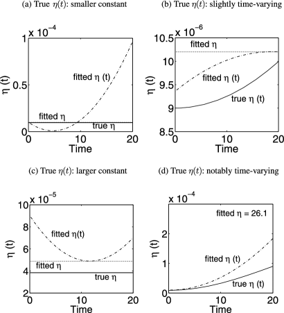
Figure 1: Simulation results for constant $\eta$ and the time-varying $\eta(t)$ models. In each figure, the true model of $\eta$ (solid), the constant $\eta$ model (dotted) and the time-varying $\eta(t)$ model (dash-dotted) are plotted and compared.

In Figure 1, the average trajectories of estimated $\eta(t)$ are compared to the true trajectories of $\eta(t)$ for four different scenarios. From this figure, we observed a similar trend as the constant parameter estimates. The misspecification of $\eta(t)$ produces estimation error, in particular for the cases with a large variation of $\eta(t)$ or a large constant $\eta$. When the model of $\eta(t)$ is correctly specified, the estimates based on the proposed methods are reasonably good. In order to evaluate the robustness of the proposed approach, we also performed further simulation studies for a complex function $\eta(t)=9.0\times 10^{-6}+9.0\times 10^{-7}\times t\times\{1-0.5\sin(\pi t/5.8)\}$ under the same simulation settings (i.e., 40 time points, 20% error, 500 simulation runs). The results suggest that the sieve estimator can still capture the essential pattern of the complex $\eta(t)$ reasonably well (plots not shown).

5.2 Application to AIDS clinical data

To illustrate applicability and feasibility of our proposed methods and theories, we also applied the proposed estimation methods to fit the HIV dynamic model to a clinical data set obtained from an HIV-1 infected patient who was treated with an antiretroviral therapy. Very frequent viral load measurements were collected from this patient after initiating the antiretroviral regimen: 13 measurements during the first day, 14 measurements from day 2 to week 2, and then one measurement at weeks 4, 8, 12, 14, 20, 24, 28, 32, 36, 40, 44, 48, 52, 56, 64, 74 and 76, respectively. In addition, the measurements of total CD4$+$ $T$ cell counts were also taken at Day 1, weeks 2 and 4, and monthly thereafter. Equation (3) was used to estimate HIV kinetic parameters using the viral load and total CD4$+$ $T$ cell data.

For simplicity of illustration and computation, we fixed the initial conditions of the state variables in (3) as $T_{U}(0)=1$, $T_{I}(0)=551$, $V(0)=6.38\times 10^{4}$, which were derived from the baseline measurements. We also fixed two parameters, as in the simulation study, $\rho=0.10$ and $\delta=0.434$, which were taken from the estimates in literature. Our objective is to estimate the three constant parameters $(\lambda,N,c)$ and the time-varying parameter $\eta(t)$ as in the simulation study. As we proposed in Section 4, we employed B-splines to approximate $\eta(t)$. We positioned the spline knots at equally-spaced time points (the log-time scale was used since the distribution of observation time points is highly-skewed). We selected the order of splines and the number of spline knots using the model selection criterion AICc given by

$$\mathrm{AICc}=n\ln\biggl{(}\frac{\mathrm{RSS}}{n}\biggr{)}+\frac{2nk}{n-k-1},$$

where RSS is the residual of the sum of squares obtained from the NLS model fitting, $n$ is the total number of observations and $k$ is the number of unknown parameters [including the coefficients in the spline representation of $\eta(t)$]. Note that as a practical guideline, if the number of unknown parameters exceeds $n/40$ (where $n$ is the sample size), the AICc instead of AIC should be used. For our clinical data, the sample size $n$ is equal to 65, and the number of unknown parameters varies between 6 and 13 for different scenarios, which is much larger than $n/40=65/40=1.6$. Thus the AICc is more appropriate for our applications. In general, the AICc converges to the AIC as the sample size gets larger, thus the AICc is often suggested to be employed regardless of the sample size [Burnham and Anderson (2004)]. For our application, we used AICc and compared the models with the splines of order 3 and 4, and the number of knots from 3 to 10. In Table 2, the AICc values for these different models are reported, from which the best model was selected as the spline with order 3 and 5 knots for $\eta(t)$ approximation.

=230pt Model Spline Number of AICc order knots 1 $3$ $-$222.3 2 $4$ $-$242.8 3 $5$ $-$252.8 4 $6$ $-$243.8 5 3 $7$ $-$250.6 6 $8$ $-$246.0 7 $9$ $-$246.8 8 $10$ $-$244.4 9 $3$ – 10 $4$ $-$233.2 11 $5$ $-$230.3 12 $6$ $-$242.6 13 4 $7$ $-$249.1 14 $8$ $-$245.5 15 $9$ $-$244.9 16 $10$ $-$240.5

Table 2: Model selection results for B-spline approximation of the time-varying parameter $\eta(t)$

We used the weighted bootstrap method to calculate both the confidence intervals for the constant parameters and the confidence bands for the time-varying parameter. The basic idea of the weighted bootstrap method is provided in Sections 3.2 and 4.2. For the computational implementation, we first generated a positive random weight for each data point in the raw data set from the exponential distribution with mean one and variance one. By repeating this step, a large number of (say, 1000) sets of weights can be generated. Second, for each set of weights, the ODE model is fitted to the data to obtain parameter estimates by minimizing the weighted residual sum of squares (see Sections 3 and 4). Recall that the time-varying parameter in the model has been approximated by B-splines, then both the constant parameters and the constant B-spline coefficients are actually estimated. Once the estimates of the B-spline coefficients are obtained, we construct the B-splines which approximate the time-varying parameter. Thus, we eventually obtain 1000 estimates for each constant parameter and 1000 B-splines for each time-varying parameter. Third, for each constant parameter, we select the 2.5% and 97.5% quantiles of the 1000 estimates to form the 95% confidence intervals for this parameter. For the time-varying parameter, at a single time point, the 1000 B-splines have 1000 values. We also select the 2.5% and 97.5% quantiles of the 1000 values at this time point to eventually form the 95% pointwise confidence bands for the time-varying parameter.

Figure 2: Model fitting results with $\eta(t)$ approximated by B-splines of order 3 and 5 knots.

=250pt Parameter Estimate 95% confidence interval $\lambda$ $46.52$ [43.20, 51.04] $N$ $1300.39$ [251.93, 4628.26] $c$ $4.35$ [0.98, 14.83]

Table 3: The constant parameter estimation results

Model fitting results are given in Figure 2 and Table 3. From Figures 2(a) and (b), we can see that the fitting is reasonably good for both CD4$+$ $T$ cell counts and viral load data. The estimates of constant parameters $(\lambda,N,c)$ are listed in Table 3, and the 95% bootstrap confidence intervals of the estimates are also provided. The uninfected cell proliferation rate ($\lambda$) was estimated as 46.52 cells per day, the average number of virions produced by one infected cell ($N$) was estimated as 1300 per day and the clearance rate of free virions was 4.35 per day which corresponds to a half-life of 3.8 hours. All these estimates are in the ballpark of similar estimates from other methods [Perelson et al. (1996, 1997)]. In Figure 2(c), the estimated trajectory of the time-varying parameter $\eta(t)$ (the viral infection rate), is plotted with 95% bootstrap quantile confidence intervals, which shows an initial fluctuation but converges to a constant after 2 to 3 months.

6 Discussion

In this paper, we have systematically studied numerical solution-based NLS estimators for general nonlinear ODE models which the closed-form solutions are not available. Both constant and time-varying parameters are considered. For the model involved time-varying parameters, we formulated the estimator under the framework of sieve approach. Our main contribution is the establishment of the asymptotic properties for the proposed numerical solution-based NLS estimators (including the sieve NLS estimator for the time-varying parameter) with consideration of both numerical error and measurement error. Our results show that if the maximum step size of the $p$-order numerical algorithm goes to zero at a rate faster than $n^{-1/(p\wedge 4)}$, the numerical error is negligible compared with the measurement error. This provides guidance in selecting the step size for numerical evaluations of ODEs. Moreover, we have shown that the numerical solution-based NLS estimator and the sieve NLS estimator for the model with a time-varying parameter are strongly consistent. The sieve estimator of constant parameters is asymptotically normal with the same asymptotic co-variance as that of the case where the true solution is exactly known, while the estimator of the time-varying parameter has an optimal convergence rate under some regularity conditions. We also obtained the theoretical results for the case when the step size of the ODE numerical solver does not go to zero fast enough or the numerical error is comparable to the measurement error [see case (ii) of Theorem 3.2 and Remark 3]. To our best knowledge, this is the first time that the sieve method has been extended to the case of ODE models which have no closed-form solutions, and the sieve-based theories were used to establish the asymptotic results and construct confidence intervals (bands) for both constant and time-varying parameters. Note that we only considered a single time-varying parameter in the model, but the methodologies can be extended to multiple time-varying parameters although it is more tedious to implement.

Note that the NLS estimators have good properties under some assumptions and are more accurate compared to other estimates such as those proposed in Ramsay et al. (2007), Chen and Wu (2008) and Liang and Wu (2008). But the price that we have to pay is the high computational cost to obtain the NLS estimates. To reduce the computational burden, we may use the rough estimates from other methods [Ramsay et al. (2007), Chen and Wu (2008), Liang and Wu (2008)] to narrow down the search range for the NLS optimization algorithm. More efficient optimization algorithms may also be employed to speed up the computation. We are also considering to parallel our global optimization algorithms on high-performance computers. Hopefully these efforts can help us to handle a reasonable size of ODE models.

This article only considered the initial value problem (IVP), that is, the initial conditions are assumed to be given. In practice, the initial conditions can be estimated from the data. However, the generalizations of the theoretical results to the cases of estimated initial conditions and other boundary value problems as well as constraints on parameters are not trivial. Also note that, if there is more than one time-varying parameter in the model, similar identifiability techniques in Section 2 may be applied to these parameters one by one, sequentially. Spline approximation to these multiple time-varying parameters can be used for estimation. But the computation and theoretical results are more complicated in this case. However, these generalizations are worth further investigations in future.

Appendix: Proofs

Lemma 1.

Under conditions A1–A5, $\sup_{t\in I}\|\tilde{\mathbf{X}}(t,\bolds\beta)-{\mathbf{X}}(t,\beta)\|_{\infty}=\break O(h^{p\wedge 4})$ for any given $\bolds\beta\in\mathcal{B}$ in (1).

By Theorem 3.4 in Hairer, Nørsett and Wanner [(1993), page 160] under conditions A1–A5, for the $p$th order numerical algorithm (12) for (1), its global discretization error satisfies

$${\max_{0\leq i\leq m-1}}\|\tilde{\mathbf{X}}(s_{i},\bolds{\beta})-\mathbf{X}(s_{i},\bolds{\beta})\|_{\infty}=O(h^{p})\qquad\mbox{for given $\bolds\beta\in\mathcal{B}$}.$$

When $t$ is not coincident with the grid points of the numerical algorithm, the cubic Hermite interpolation [de Boor (1978), page 51] will be used to obtain the solution at time $t$. In this case,

$${\sup_{t\in I\setminus\{s_{i}\dvtx 0\leq i\leq m-1\}}}\|\tilde{\mathbf{X}}(t,\bolds{\beta})-\mathbf{X}(t,\bolds{\beta})\|_{\infty}=O(h^{4}).$$

Then it follows that

$$\sup_{t\in I}\|\tilde{\mathbf{X}}(t,\bolds{\beta})-\mathbf{X}(t,\bolds{\beta})\|_{\infty}$$

$$\qquad\leq{\sup_{t\in I\setminus\{s_{i}\dvtx 0\leq i\leq m-1\}}}\|\tilde{\mathbf{X}}(t,\bolds{\beta})-\mathbf{X}(t,\bolds{\beta})\|_{\infty}$$

$$\qquad\quad{}+{\max_{t\in\{s_{i}\dvtx 0\leq i\leq m-1\}}}\|\tilde{\mathbf{X}}(t,\bolds{\beta})-\mathbf{X}(t,\bolds{\beta})\|_{\infty}$$

$$\qquad=O(h^{4})+O(h^{p}).$$

In general, $h$ is less than 1, $O(h^{4})+O(h^{p})=O(h^{p\wedge 4})$, which completes the proof.

Moreover, Lemma 1 can be extended to the ODE model (2) with both constant and time-varying parameters, since for this model, it can be verified that the result of Theorem 3.1 in Hairer, Nørsett and Wanner [(1993), page 157] is still valid for any given $\bolds\beta\in\mathcal{B}$ and $\eta\in\mathcal{A}$ under condition B2 (it can be derived using the Taylor expansion and the Chain rule), which leads to the same conclusion as Theorem 3.4 in Hairer, Nørsett and Wanner [(1993), page 160]. For Theorems 3.1 and 3.2, the proofs for the univariate and multivariate cases are the same. For presentation and notation simplicity, we only outline the proof for the univariate case below. Proof of Theorem 3.1 Denote $\tilde{M}_{n}(\bolds\beta)=\frac{1}{n}\sum_{i=1}^{n}[Y(t_{i})-\tilde{X}(t_{i},\bolds\beta)]^{2}$, $M_{n}(\bolds\beta)=\frac{1}{n}\sum_{i=1}^{n}[Y(t_{i})-X(t_{i},\bolds\beta)]^{2}$ and $M(\bolds\beta)=[Y(t)-X(t,\bolds\beta)]^{2}$.

First, we claim that $E_{0}[M(\bolds\beta)]$ reaches its unique minimum at $\bolds\beta=\bolds{\beta}_{0}$. In fact,

$$E_{0}[M(\bolds\beta)] = E_{0}[Y(t)-X(t,\bolds\beta)]^{2}$$

$$= E_{0}[Y(t)-X(t,\bolds{\beta}_{0})+X(t,\bolds{\beta}_{0})-X(t,\bolds\beta)]^{2}$$

$$= E_{0}[Y(t)-X(t,\bolds{\beta}_{0})]^{2}+E_{t}[X(t,\bolds{\beta}_{0})-X(t,\bolds\beta)]^{2}$$

$$= E_{0}[\varepsilon(t)]^{2}+E_{t}[X(t,\bolds{\beta}_{0})-X(t,\bolds\beta)]^{2}$$

$$\geq E_{0}[\varepsilon(t)]^{2}=E_{0}[M(\bolds{\beta}_{0})],$$

where the third equality holds because the intersection term equals zero according to the following calculation:

$$E_{0}[\varepsilon(t)][X(t,\bolds{\beta}_{0})-X(t,\bolds\beta)]$$

$$\qquad=E_{t}E_{0}\{[\varepsilon(t)][X(t,\bolds{\beta}_{0})-X(t,\bolds\beta)]|t\}$$

$$\qquad=E_{t}\{[X(t,\bolds{\beta}_{0})-X(t,\bolds\beta)]E_{0}[\varepsilon(t)]\}$$

$$\qquad=0,$$

because of $E_{0}[\varepsilon(t)]=0$. Moreover, $E_{t}[X(t,\bolds{\beta})-X(t,\bolds{\beta}_{0})]^{2}=0$ if and only if $\bolds{\beta}=\bolds{\beta}_{0}$ from assumption A6. Thus the above claim holds. Under assumption A10, it follows that the first-order derivative $\frac{\partial E_{0}[M(\bolds\beta)]}{\partial\bolds\beta}$ of $E_{0}[M(\bolds\beta)]$ at $\bolds{\beta}_{0}$ equals to zero and the second-order derivative $\frac{\partial^{2}E_{0}[M(\bolds\beta)]}{\partial\bolds\beta\,\partial\bolds\beta^{T}}$ of $E_{0}[M(\bolds\beta)]$ at $\bolds{\beta}_{0}$ is positive definite. By assumptions A7 and A9, the second-order derivative of $E_{0}[M(\bolds\beta)]$ in a small neighborhood of $\bolds{\beta}_{0}$ is bounded away from 0 and $\infty$. Then the second-order Taylor expansion of $E_{0}[M(\bolds\beta)]$ gives that there exists a constant $0<C<\infty$ such that

$$E_{0}[M(\hat{\bolds{\beta}}_{n})-M(\bolds{\beta}_{0})]\geq C\|\hat{\bolds{\beta}}_{n}-\bolds{\beta}_{0}\|^{2}.$$

Thus it is sufficient to prove $E_{0}[M(\bolds{\beta}_{0})]-E_{0}[M(\hat{\bolds{\beta}}_{n})]\rightarrow 0$, a.s.

Let $N_{1}(\varepsilon,\mathcal{Q},\mathcal{F})$ be the covering number of the class $\mathcal{F}$ in the probability measure $\mathcal{Q}$, as given in Pollard (1984, page 25). From Lemma 4.1 in Pollard (1990), we have that $N_{1}(\varepsilon,L_{2},\mathcal{B})\leq(\frac{3R_{\bolds\beta}}{\varepsilon})^{d}$. Let $\mathcal{F}_{n}$ be the set $\{M_{n}(\bolds\beta)\dvtx\bolds\beta\in\mathcal{B}\}$. With the Taylor expansion, for any $\bolds{\beta}_{1}$, $\bolds{\beta}_{2}\in\mathcal{B}$, we can easily obtain

$$|M_{n}(\bolds{\beta}_{1})-M_{n}(\bolds{\beta}_{2})|\leq C\|\bolds{\beta}_{1}-\bolds{\beta}_{2}\|,$$

where $C$ is some constant. Then for any probability measure $Q$, we have

$$\sup_{Q}N_{1}(\varepsilon,Q,\mathcal{F}_{n})\leq N_{1}(\varepsilon/C,L_{2},\mathcal{B})\leq C\biggl{(}\frac{1}{\varepsilon}\biggr{)}^{d}\qquad\mbox{for $0<\varepsilon<1$}.$$

Then by Theorem II.37 in Pollard (1984), $\sup_{\bolds\beta}|M_{n}(\beta)-E_{0}M(\bolds\beta)|\rightarrow 0$, a.s., under $P_{\bolds{\beta}_{0}}$. Then we have $M_{n}(\hat{\bolds{\beta}}_{n})-E_{0}[M(\hat{\beta}_{n})]\rightarrow 0$ and $M_{n}(\bolds{\beta}_{0})-E_{0}[M(\bolds{\beta}_{0})]\rightarrow 0$, a.s.

Next, by Lemma 1,

$$\tilde{M}_{n}(\bolds\beta) = \frac{1}{n}\sum_{i=1}^{n}[Y(t_{i})-\tilde{X}(t_{i},\bolds\beta)]^{2}$$

$$= \frac{1}{n}\sum_{i=1}^{n}\bigl{[}Y(t_{i})-X(t_{i},\bolds\beta)+O\bigl{(}n^{-\lambda(p\wedge 4)}\bigr{)}\bigr{]}^{2}$$

$$= \frac{1}{n}\sum_{i=1}^{n}[Y(t_{i})-X(t_{i},\bolds\beta)]^{2}+O\bigl{(}n^{-\lambda(p\wedge 4)}\bigr{)}$$

$$= M_{n}(\bolds\beta)+O\bigl{(}n^{-\lambda(p\wedge 4)}\bigr{)}.$$

Then

$$\tilde{M}_{n}(\hat{\bolds{\beta}}_{n})-E_{0}[M(\bolds{\beta}_{0})]$$

$$\qquad\geq\tilde{M}_{n}(\hat{\bolds{\beta}}_{n})-E_{0}[M(\hat{\bolds{\beta}}_{n})]$$

$$\qquad=M_{n}(\hat{\bolds{\beta}}_{n})+O\bigl{(}n^{-\lambda(p\wedge 4)}\bigr{)}-E_{0}[M(\hat{\bolds{\beta}}_{n})]$$

and

$$\tilde{M}_{n}(\hat{\bolds{\beta}}_{n})-E_{0}[M(\bolds{\beta}_{0})]$$

$$\qquad\leq\tilde{M}_{n}(\bolds{\beta}_{0})-E_{0}[M(\bolds{\beta}_{0})]$$

$$\qquad=M_{n}(\bolds{\beta}_{0})+O\bigl{(}n^{-\lambda(p\wedge 4)}\bigr{)}-E_{0}M(\bolds{\beta}_{0}).$$

Hence $\tilde{M}_{n}(\hat{\bolds{\beta}}_{n})-E_{0}[M(\bolds{\beta}_{0})]\rightarrow 0$, a.s. Thus

$$|E_{0}[M(\hat{\bolds{\beta}}_{n})]-E_{0}[M(\bolds{\beta}_{0})]|$$

$$\qquad\leq|\tilde{M}_{n}(\hat{\bolds{\beta}}_{n})-E_{0}[M(\hat{\bolds{\beta}}_{n})]|+|\tilde{M}_{n}(\hat{\bolds{\beta}}_{n})-E_{0}[M(\bolds{\beta}_{0})]|\rightarrow 0\qquad\mbox{a.s.}$$

Since $\bolds{\beta}_{0}$ is the unique minimum point for $E_{0}[M(\bolds\beta)]$, $\hat{\bolds{\beta}}_{n}$ is almost surely consistent with respect to $P_{\bolds{\beta}_{0}}$. Proof of Theorem 3.2 For the proof of part (i), it suffices to verify conditions of Theorem 2 in Pollard (1985). Denote $\tilde{G}_{n}(\bolds\beta)=\frac{1}{n}\sum_{i=1}^{n}[Y(t_{i})-\tilde{X}(t_{i},\bolds\beta)]\frac{\partial\tilde{X}(t_{i},\bolds\beta)}{\partial\bolds\beta}$, $G_{n}(\bolds\beta)=\frac{1}{n}\sum_{i=1}^{n}[Y(t_{i})-X(t_{i},\bolds\beta)]\,\frac{\partial X(t_{i},\bolds\beta)}{\partial\bolds\beta}$ and $G(\bolds\beta)=\break E_{0}[Y(t)-X(t,\bolds\beta)]\,\frac{\partial X(t,\bolds\beta)}{\partial\bolds\beta}$. Obviously, $\tilde{G}_{n}(\hat{\bolds{\beta}}_{n})=0$ and $G(\bolds{\beta}_{0})=E_{t}E_{0}(\{[Y(t)-X(t,\bolds{\beta}_{0})]\,\frac{\partial X(t,\bolds{\beta}_{0})}{\partial\bolds{\beta}_{0}}\}|t)=0$ from $E_{0}[Y(t)|t]=X(t,\bolds{\beta}_{0})$.

First, we verify the following result: $\sqrt{n}[\tilde{G}_{n}(\bolds{\beta}_{0})-G(\bolds{\beta}_{0})]\stackrel{{\scriptstyle d}}{{\rightarrow}}N(0,H_{1})$. For fixed $t$, according to the multivariate inequality of Kolmogorov type for $L_{2}$-norms of derivatives [Babenko, Kofanov and Pichugov (1996), page 9], we have $\|\frac{\partial\tilde{\mathbf{X}}(t,\bolds\beta)}{\partial\bolds\beta}-\frac{\partial{\mathbf{X}}(t,\bolds\beta)}{\partial\bolds\beta}\|\leq C\|\frac{\partial^{2}\tilde{\mathbf{X}}(t,\bolds\beta)}{\partial\bolds\beta\,\partial\bolds\beta^{T}}-\frac{\partial^{2}{\mathbf{X}}(t,\bolds\beta)}{\partial\bolds\beta\,\partial\bolds\beta^{T}}\|_{\infty}^{1/2}\|\tilde{\mathbf{X}}(t,\bolds\beta)-{\mathbf{X}}(t,\bolds\beta)\|_{\infty}^{1/2}\leq C^{\prime}\|\tilde{\mathbf{X}}(t,\bolds\beta)-{\mathbf{X}}(t,\bolds\beta)\|_{\infty}^{1/2}$ for two constants $C$ and $C^{\prime}$, where the second inequality holds because of the uniform boundedness of both $\frac{\partial^{2}{\mathbf{X}}(t,\bolds\beta)}{\partial\bolds\beta\,\partial\bolds\beta^{T}}$ and $\frac{\partial^{2}\tilde{\mathbf{X}}(t,\bolds\beta)}{\partial\bolds\beta\,\partial\bolds\beta^{T}}$ under conditions A7 and A8. Based on $\sup_{t\in I}\|\tilde{\mathbf{X}}(t,\bolds\beta)-{\mathbf{X}}(t,\beta)\|_{\infty}=O(n^{-\lambda(p\wedge 4)})$ from Lemma 1, it follows that $\|\frac{\partial\tilde{\mathbf{X}}(t,\bolds\beta)}{\partial\bolds\beta}-\frac{\partial{\mathbf{X}}(t,\bolds\beta)}{\partial\bolds\beta}\|=O(n^{-\lambda(p\wedge 4)/2})$. Considering that $Y(t_{i})-X(t_{i},\bolds{\beta}_{0})$ and $\frac{\partial\tilde{X}(t_{i},\bolds{\beta}_{0})}{\partial\bolds\beta_{0}}$ are bounded, we have

$$\sqrt{n}[\tilde{G}_{n}(\bolds{\beta}_{0})-G(\bolds{\beta}_{0})]$$

$$\qquad=\frac{1}{\sqrt{n}}\sum_{i=1}^{n}[Y(t_{i})-\tilde{X}(t_{i},\bolds{\beta}_{0})]\,\frac{\partial\tilde{X}(t_{i},\bolds{\beta}_{0})}{\partial\bolds\beta_{0}}$$

$$\qquad=\frac{1}{\sqrt{n}}\sum_{i=1}^{n}\bigl{[}Y(t_{i})-X(t_{i},\bolds{\beta}_{0})+O\bigl{(}n^{-\lambda(p\wedge 4)}\bigr{)}\bigr{]}\biggl{[}\frac{\partial X(t_{i},\bolds{\beta}_{0})}{\partial\bolds{\beta}_{0}}+O\bigl{(}n^{-\lambda(p\wedge 4)/2}\bigr{)}\biggr{]}$$

$$\qquad=\frac{1}{\sqrt{n}}\sum_{i=1}^{n}[Y(t_{i})-X(t_{i},\bolds{\beta}_{0})]\,\frac{\partial X(t_{i},\bolds{\beta}_{0})}{\partial\bolds{\beta}_{0}}+O\bigl{(}n^{-\lambda(p\wedge 4)/2+1/2}\bigr{)}.$$

When $\lambda>1/(p\wedge 4)$, $O(n^{-\lambda(p\wedge 4)/2+1/2})=o(1)$. So for the above expression, we have

$$\sqrt{n}[\tilde{G}_{n}(\bolds{\beta}_{0})-G(\bolds{\beta}_{0})]$$

$$\qquad=\frac{1}{\sqrt{n}}\sum_{i=1}^{n}[Y(t_{i})-X(t_{i},\bolds{\beta}_{0})]\,\frac{\partial X(t_{i},\bolds{\beta}_{0})}{\partial\bolds{\beta}_{0}}+o(1)$$

$$\qquad=\sqrt{n}[G_{n}(\bolds{\beta}_{0})-G(\bolds{\beta}_{0})]+o(1).$$

Based on the general central limit theorem, $\sqrt{n}[G_{n}(\bolds{\beta}_{0})-G(\bolds{\beta}_{0})]\rightarrow N(0,\mathbf{H}_{1})$ with

$$\mathbf{H}_{1}=E_{0}[Y(t)-X(t,\bolds{\beta}_{0})]^{2}\biggl{[}\frac{\partial X(t,\bolds{\beta}_{0})}{\partial\bolds{\beta}_{0}}\biggr{]}^{\otimes 2}=\sigma_{0}^{2}E_{t}\biggl{[}\frac{\partial X(t,\bolds{\beta}_{0})}{\partial\bolds{\beta}_{0}}\biggr{]}^{\otimes 2}.$$

Second, let $\delta_{n}\downarrow 0$. For $\|\bolds\beta-\bolds{\beta}_{0}\|\leq\delta_{n}$, we want to show that

$$\sqrt{n}[\tilde{G}_{n}(\bolds\beta)-G(\bolds\beta)]-\sqrt{n}[\tilde{G}_{n}(\bolds{\beta}_{0})-G(\bolds{\beta}_{0})]=o_{p}(1).$$

In fact, from the first step above, for any $\bolds\beta\in\mathcal{B}$, we have that $\sqrt{n}[\tilde{G}_{n}(\bolds\beta)-G_{n}(\bolds\beta)]=o_{p}(1)$. Then

$$\sqrt{n}[\tilde{G}_{n}(\bolds\beta)-G(\bolds\beta)]-\sqrt{n}[\tilde{G}_{n}(\bolds{\beta}_{0})-G(\bolds{\beta}_{0})]$$

$$\qquad=\sqrt{n}[G_{n}(\bolds\beta)-G(\bolds\beta)]-\sqrt{n}[G_{n}(\bolds{\beta}_{0})-G(\bolds{\beta}_{0})]+o_{p}(1).$$

From Lemma 4.1 in Pollard (1990), we have that $N_{1}(\varepsilon,L_{2},\mathcal{B})\leq(\frac{3R}{\varepsilon})^{d}$. Let $\Lambda_{n}$ be the set $\{G_{n}(\bolds\beta)\dvtx\bolds\beta\in\mathcal{B}\}$ for any $X\in\mathcal{X}$. Using a Taylor series expansion, for any $\bolds{\beta}_{1}$, $\bolds{\beta}_{2}\in\mathcal{B}$, we can easily obtain

$$|G_{n}(\bolds{\beta}_{1})-G_{n}(\bolds{\beta}_{2})|\leq C\|\bolds{\beta}_{1}-\bolds{\beta}_{2}\|,$$

where $C$ is some constant. Then for any probability measure $Q$, we have

$$N_{1}(\varepsilon,L_{2}(Q),\Lambda_{n})\leq N_{1}(\varepsilon/C,L_{2},\mathcal{B})\leq C\biggl{(}\frac{1}{\varepsilon}\biggr{)}^{d},$$

and thus

$$\log N_{1}(\varepsilon,L_{2}(Q),\Lambda_{n})\leq d\log{\frac{1}{\varepsilon}}.$$

Since $\int_{0}^{1}\log(1/\varepsilon)\,d\varepsilon<\infty$, $\Lambda_{n}$ is a P-Donsker class by Theorem 2.5.2 in van der Vaart and Wellner (1996). Hence $\sqrt{n}[G_{n}(\bolds\beta)-G(\bolds\beta)]-\sqrt{n}[G_{n}(\bolds{\beta}_{0})-G(\bolds{\beta}_{0})]=o_{p}(1)$.

Third, with some simple calculations, we have $G(\bolds\beta)=E_{t}[X(t,\bolds{\beta}_{0})-X(t$,$\bolds\beta)]\,\frac{\partial X(t,\bolds\beta)}{\partial\bolds\beta}$, then

$$\frac{\partial G(\bolds\beta)}{\partial\bolds\beta}=-\int\biggl{\{}\frac{\partial X(t,\bolds\beta)}{\partial\bolds\beta}\biggr{\}}^{\otimes 2}\,d\Phi(t)+\int[X(t,\bolds{\beta}_{0})-X(t,\bolds\beta)]\,\frac{\partial^{2}X(t,\bolds\beta)}{\partial\bolds\beta\,\partial\bolds\beta^{T}}\,d\Phi(t)$$

and $\frac{\partial G(\bolds\beta)}{\partial\bolds\beta}|_{\bolds\beta=\bolds{\beta}_{0}}=-E_{t}\{\frac{\partial X(t,\bolds{\beta}_{0})}{\partial\bolds{\beta}_{0}}\}^{\otimes 2}$. Denote $\mathbf{H}_{2}=E_{t}\{\frac{\partial X(t,\bolds{\beta}_{0})}{\partial\bolds{\beta}_{0}}\}^{\otimes 2}$. Then by using the Taylor series expansion again, the function $G(\bolds\beta)$ isFréchet-differentiable at $\bolds\beta_{0}$ with nonsingular derivative $\mathbf{H}_{2}$.

Thus all conditions of Theorem 2 in Pollard (1985) are satisfied, then Theorem 3.2(i) holds with $\mathbf{V}_{1}=\mathbf{H}_{2}^{-1}\mathbf{H}_{1}(\mathbf{H}_{2}^{-1})^{T}=\sigma_{0}^{2}\{E_{t}[\frac{\partial X(t,\bolds{\beta}_{0})}{\partial\bolds{\beta}_{0}}]^{\otimes 2}\}^{-1}$.

For the proof of case (ii) of Theorem 3.2, it is easy to verify the conditions of Theorem 2 in Pollard (1985) for the asymptotic normality. Now we just need to show $\tilde{\bolds\beta}=\bolds\beta_{0}+O(h^{(p\wedge 4)/2})$ and $\tilde{V}_{1}=V_{1}+O(h^{(p\wedge 4)/2})$. Denote $\tilde{M}(\bolds\beta)=[Y(t)-\tilde{X}(t,\bolds\beta)]^{2}$ and $\tilde{G}(\bolds\beta)=E_{0}[Y(t)-\tilde{X}(t,\beta)]\,\frac{\partial\tilde{X}(t,\bolds\beta)}{\partial\bolds\beta}$. Since $E_{0}[\tilde{M}(\bolds\beta)]$ reaches its minimum at $\bolds\beta=\tilde{\bolds\beta}$, then the first-order derivative of $E_{0}[\tilde{M}(\bolds\beta)]$ at $\tilde{\bolds\beta}$ equals 0, that is, $\tilde{G}(\tilde{\bolds\beta})=0$. Then similar to the proof of case (i) above, we have

$$\tilde{G}(\bolds\beta) = E_{0}[Y(t)-\tilde{X}(t,\bolds\beta)]\,\frac{\partial\tilde{X}(t,\bolds\beta)}{\partial\bolds\beta}$$

$$= E_{0}[Y(t)-X(t,\bolds\beta)+O(h^{p\wedge 4})]\biggl{[}\frac{\partial X(t,\bolds\beta)}{\partial\bolds\beta}+O\bigl{(}h^{(p\wedge 4)/2}\bigr{)}\biggr{]}$$

$$= G(\bolds\beta)+O\bigl{(}h^{(p\wedge 4)/2}\bigr{)}.$$

It follows that $\tilde{G}(\tilde{\bolds\beta})=G(\tilde{\bolds\beta})+O(h^{(p\wedge 4)/2})$, then $G(\tilde{\bolds\beta})=O(h^{(p\wedge 4)/2})$ from $\tilde{G}(\tilde{\bolds\beta})=0$. The Taylor series expansion yields that there exist constants $0<c_{1},c_{2}<\infty$ such that

$$c_{1}\|\tilde{\bolds\beta}-\bolds\beta_{0}\|\leq|G(\tilde{\bolds\beta})-G(\bolds\beta_{0})|\leq c_{2}\|\tilde{\bolds\beta}-\bolds\beta_{0}\|.$$

Thus $\|\tilde{\bolds\beta}-\bolds\beta_{0}\|=O(h^{(p\wedge 4)/2})$ from $G(\bolds\beta_{0})=0$. Similarly we can show that $\|\tilde{\mathbf{V}}_{1}-\mathbf{V}_{1}\|=O(h^{(p\wedge 4)/2})$.

Some definitions and notation are necessary in order to prove Theorems 4.1–4.3. Denote $\tilde{M}_{n}(\bolds\theta)=\frac{1}{n}\sum_{i=1}^{n}\sum_{j=1}^{K}[Y_{j}(t_{i})-\tilde{\mathbf{X}}_{j}(t_{i},\bolds\beta,\eta(t_{i}))]^{2}$, $M_{n}(\bolds\theta)=\frac{1}{n}\sum_{i=1}^{n}\sum_{j=1}^{K}[Y_{j}(t_{i})-\mathbf{X}_{j}(t_{i},\bolds\beta,\eta(t_{i}))]^{2}$ and $M(\bolds\theta)=\sum_{j=1}^{K}[Y_{j}-\mathbf{X}_{j}(t,\bolds\beta,\eta(t))]^{2}$. We define a semidistance $\rho$ on $\Theta$ as

$$\rho^{2}(\bolds\theta,\bolds{\theta}_{0})=E_{0}\{(\bolds\beta-\bolds{\beta}_{0})^{T}\dot{M}_{1}(\bolds\theta)+\dot{M}_{2}(\bolds\theta)[\eta-\eta_{0}]\}^{2},$$

where $\dot{M}_{1}$ is the score function of $M$ for $\bolds\beta$, and $\dot{M}_{2}$ is the score operator of $M$ for $\eta$, both evaluated at the true parameter value $\bolds{\theta}_{0}$. Similarly to the proof in Huang and Rossini [(1997), page 966] when $\mathbf{V}_{2}(\bolds{\theta}_{0})$, defined in assumption B6, is positive definite, and $\dot{M}_{1}$ and $\dot{M}_{2}$ are bounded away from $+\infty$ and $-\infty$, if $\rho(\hat{\bolds{\theta}}_{n},\bolds{\theta}_{0})=O_{p}(r_{n})$, then $d(\hat{\bolds{\theta}}_{n},\bolds{\theta}_{0})=O_{p}(r_{n})$; and if $\rho(\hat{\bolds{\theta}}_{n},\bolds{\theta}_{0})\rightarrow 0$ almost surely under $P_{\bolds{\theta}_{0}}$, then $d(\hat{\bolds{\theta}}_{n},\bolds{\theta}_{0})\rightarrow 0$ almost surely under $P_{\bolds{\theta}_{0}}$. Proof of Theorem 4.1 Similarly to the proof of Theorem 3.1, we have that $E_{0}[M(\bolds{\theta}_{0})]$ reaches its unique minimum at $\bolds\theta=\bolds\theta_{0}$. It follows that

$$E_{0}[M(\bolds{\theta}_{0})-M(\hat{\bolds{\theta}}_{n})]\geq C\rho^{2}(\hat{\bolds{\theta}}_{n},\bolds{\theta}_{0}),$$

where $C$ is some constant. Thus if $E_{0}[M(\bolds{\theta}_{0})]-E_{0}[M(\hat{\bolds{\theta}}_{n})]\rightarrow 0$, almost surely under $P_{\bolds{\theta}_{0}}$, then $d(\hat{\bolds{\theta}}_{n},\bolds{\theta}_{0})\rightarrow 0$, almost surely under $P_{\bolds{\theta}_{0}}$.

Let $\mathcal{A}_{n}^{\delta}$ be the set $\{\eta\in\mathcal{A}_{n},\|\eta-\eta_{n0}\|_{2}\leq\delta\}$ and $N_{2}(\varepsilon,L_{\infty},\mathcal{A}_{n}^{\delta})$ be its bracketing number with respect to $L_{\infty}$ [see Definition 2.1.6, van der Vaart and Wellner (1996)], where $\eta_{n0}$ is the map point of $\eta_{0}$ in the sieve $\mathcal{A}_{n}$. By the calculation of Shen and Wong [(1994), page 597] for any $\varepsilon\leq\delta$, we have

$$N_{2}(\varepsilon,L_{\infty},\mathcal{A}_{n}^{\delta})\leq C(\delta/\varepsilon)^{N},$$

where $N=q+l$ is the number of B-splines basis functions. Let $\mathcal{F}_{n}$ be the set $\{M_{n}(\bolds\theta)\dvtx\|\bolds\beta-\bolds{\beta}_{0}\|\leq\delta,\eta\in\mathcal{A}_{n},\|\eta-\eta_{n0}\|_{2}\leq\delta\}$. For any $\bolds{\theta}_{1}$, $\bolds{\theta}_{2}\in\Theta_{n}$, we can easily obtain

$$|M_{n}(\bolds{\theta}_{1})-M_{n}(\bolds{\theta}_{2})|\leq C(\|\bolds{\beta}_{1}-\bolds{\beta}_{2}\|+\|\eta_{1}-\eta_{2}\|_{\infty})$$

using Taylor’s expansion. Hence

$$N_{2}(\varepsilon,L_{\infty},\mathcal{F}_{n}) \leq N_{1}(\varepsilon/2,L_{2},\mathcal{B})\times N_{2}(\varepsilon/2,L_{\infty},\mathcal{A}_{n}^{\delta})$$

$$\leq C(3R_{d}/\varepsilon)^{d}(\delta/\varepsilon)^{N}$$

$$\leq C^{\prime}(1/\varepsilon)^{N+d}.$$

Note that, since $N_{2}(\varepsilon,L_{\infty},\mathcal{F}_{n})$ depends on $n$ in the above expression, we cannot directly use Theorem II.37 in Pollard (1984) to obtain ${\sup_{\mathcal{F}_{n}}}|M_{n}(\bolds\theta)-E_{0}[M(\bolds\theta)]|\rightarrow 0$, a.s., under $P_{\bolds{\theta}_{0}}$. Fortunately, we can still get this result based on (A.2) in Xue, Lam and Li (2004). Thus we have $M_{n}(\hat{\bolds{\theta}}_{n})-E_{0}[M(\hat{\bolds{\theta}}_{n})]\rightarrow 0$ and $M_{n}(\bolds{\theta}_{n0})-E_{0}[M(\bolds{\theta}_{n0})]\rightarrow 0$, a.s., where $\bolds{\theta}_{n0}$ is the map point of $\bolds{\theta}_{0}$ in the sieve $\Theta_{n}$.

From the extension of Lemma 1 for any given $\bolds\beta\in\mathcal{B}$ and $\eta(t)\in\mathcal{A}$ in (2), similarly to (Appendix: Proofs), we have

$$\tilde{M}_{n}(\bolds\theta)=M_{n}(\bolds\theta)+O\bigl{(}n^{-\lambda(p\wedge 4)}\bigr{)}.$$ (19)

Then the remaining steps are similar to those in the proof of Theorem 3.1. Proof of Theorem 4.2 We apply Theorem 3.4.1 in van der Vaart and Wellner (1996) to obtain the rate of convergence.

For $\bolds\theta_{n0}$ in the proof of Theorem 4.1, define $\bolds\theta_{n0}\mapsto\rho_{1}(\bolds\theta,\bolds\theta_{n0})$ be a map from $\Theta_{n}$ to $[0,\infty)$ as $\rho_{1}^{2}(\bolds\theta,\bolds\theta_{n0})=E_{0}[M(\bolds\theta)]-E_{0}[M(\bolds\theta_{n0})]$. Choose $\delta_{n}=\rho(\bolds\theta_{0},\bolds\theta_{n0})$. For $\delta_{n}<\delta<\infty$, denote $\Omega=\{\bolds\theta\dvtx\bolds\theta\in\Theta_{n},\delta/2<\rho(\bolds\theta,\bolds\theta_{n0})\leq\delta\}$. From the definition of $\rho_{1}$, we have $\sup_{\Omega}E_{0}[M(\bolds\theta_{n0})]-E_{0}[M(\bolds\theta)]\leq-\frac{\delta^{2}}{4}$.

Let $\Xi_{n}$ be the set $\{M_{n}(\bolds\theta)-M(\bolds\theta_{n0})\dvtx\bolds\theta\in\Theta_{n}\}$ and $\tilde{J}(\delta,L_{2}(P),\Xi_{n})$ be the $L_{2}(P)$-norm bracketing integral of the sieve $\Theta_{n}$. From the proof of Theorem 4.1, we have

$$\tilde{J}(\delta,L_{2}(P),\Xi_{n}) = \int_{0}^{\delta}\sqrt{1+\log N_{2}(\varepsilon,L_{2}(P),\Xi_{n})}\,d\varepsilon$$

$$\leq \int_{0}^{\delta}\sqrt{1+\log N_{2}(\varepsilon,L_{\infty},\Xi_{n})}\,d\varepsilon$$

$$\leq CN^{1/2}\delta.$$

Let

$$\phi_{n}(\delta)=\tilde{J}(\delta,L_{2}(P),\Xi_{n})\biggl{(}1+\frac{\tilde{J}(\delta,L_{2}(P),\Xi_{n})}{\delta^{2}\sqrt{n}}\biggr{)}=N^{1/2}\delta+\frac{N}{\sqrt{n}}.$$

Obviously, $\phi_{n}(\delta)/\delta^{1+\tau}$ is a decreasing function in $\delta$ for $0<\tau<1$. Then by Lemma 3.4.2 in van der Vaart and Wellner (1996), we have

$$E_{0}\Bigl{[}\sup_{\Omega}\sqrt{n}(M_{n}-M)(\bolds\theta-\bolds\theta_{n0})\Bigr{]}\preceq\phi_{n}(\delta).$$

For $\lambda>1/[2(p\wedge 4)]$, from (19), it follows that

$$\sqrt{n}[\tilde{M}_{n}(\bolds\theta)-M_{n}(\bolds\theta)]=O\bigl{(}n^{1/2-\lambda(p\wedge 4)}\bigr{)}=o(1).$$

Then we have that

$$E_{0}\Bigl{[}\sup_{\Omega}\sqrt{n}(\tilde{M}_{n}-M)(\bolds\theta-\bolds\theta_{n0})\Bigr{]}\preceq\phi_{n}(\delta).$$

Then the conditions of Theorem 3.4.1 in van der Vaart and Wellner (1996) are satisfied for the $\delta_{n}$, $\rho_{1}$ and $\phi_{n}(\delta)$ above. Therefore we have $-r_{n}^{2}\rho_{1}(\hat{\bolds{\theta}}_{n},\bolds\theta_{n0})=O_{p}(1)$, where $r_{n}$ satisfies $r_{n}^{2}\phi_{n}(\frac{1}{r_{n}})\leq\sqrt{n}$. It follows that $r_{n}=N^{-1/2}n^{1/2}=n^{(1-v)/2}$. Thus $\rho_{1}(\hat{\bolds{\theta}}_{n},\bolds\theta_{n0})=O_{p}(n^{-(1-v)/2})$.

Now, we define a distance $\rho_{2}$ as

$$\rho_{2}(\bolds\theta_{1},\bolds\theta_{2})=\|\bolds\beta_{1}-\bolds\beta_{2}\|+\|\eta_{1}-\eta_{2}\|_{\infty}.$$

Let $\varsigma$ be a positive constant. Similarly to the proof of Theorem 3.2 in Huang (1999), it is easy to follow that for any $\bolds\theta$ with $\rho_{2}(\bolds\theta,\bolds\theta_{n0})\leq\varsigma$, there exist constants $0<c_{1},c_{2}<\infty$ such that

$$-c_{1}d^{2}(\bolds\theta,\bolds\theta_{n0})+O_{p}(n^{-2v\varrho})\leq-\rho^{2}_{1}(\bolds\theta,\bolds\theta_{n0})\leq-c_{2}d^{2}(\bolds\theta,\bolds\theta_{n0})+O_{p}(n^{-2v\varrho}).$$

Therefore, for a constant $c_{2}>0$,

$$c_{2}d^{2}(\hat{\bolds\theta}_{n},\bolds\theta_{n0})\leq O_{p}\bigl{(}n^{-2v\varrho}+n^{-(1-v)}\bigr{)}.$$

Because $d(\bolds\theta_{n0},\bolds\theta_{0})\leq\rho_{2}(\bolds\theta_{0},\bolds\theta_{0})=O_{p}(n^{-v\varrho})$, we have $d(\hat{\bolds\theta}_{n},\bolds\theta_{0})=O_{p}(n^{-v\varrho}+n^{-(1-v)/2})$. Proof of Theorem 4.3 We prove this theorem using Theorem 6.1 in Wellner and Zhang (2007). It suffices to validate conditions A1–A6 of Theorem 6.1 in Wellner and Zhang (2007). From the proof of Theorems 4.1 and 4.2 above, it is easy to see that condition A1 regarding consistency and rate of convergence and condition A2 for Theorem 6.1 in Wellner and Zhang (2007) hold.

For condition A3, we need to calculate the pseudo-information matrix. For any fixed $\eta\in\mathcal{A}$, let $\mathcal{A}_{0}=\{\eta_{\omega}(\cdot)\dvtx\omega$ in a neighborhood of $0\in\mathcal{R}\}$ be a smooth curve in $\mathcal{A}$ running through $\eta_{0}$ at $\omega=0$, that is, $\eta_{\omega=0}(t)=\eta_{0}(t)$. Denote $\frac{\partial}{\partial\omega}\,\eta_{\omega}(t)|_{\omega=0}=a(t)$ and the space generated by such $a(t)$ as $\Upsilon$. The score functions of $\bolds\beta$ and $\eta$ are

$$\dot{M}_{1} = \frac{\partial M}{\partial\bolds\beta}=-2\sum_{j=1}^{K}(Y_{j}-\mathbf{X}_{j})\,\frac{\partial\mathbf{X}_{j}}{\partial\bolds\beta_{0}},$$

$$\dot{M}_{2}[a] = \frac{\partial M}{\partial\eta_{0}}=-2\sum_{j=1}^{K}(Y_{j}-\mathbf{X}_{j})\,\frac{\partial\mathbf{X}_{j}}{\partial\eta_{0}}a(t).$$

We also set

$$\dot{M}_{11} = \frac{\partial^{2}M}{\partial\bolds\beta_{0}\,\partial\bolds\beta_{0}^{T}}=2\sum_{j=1}^{K}\biggl{[}\frac{\partial\mathbf{X}_{j}}{\partial\bolds\beta_{0}}\,\frac{\partial\mathbf{X}_{j}}{\partial\bolds\beta_{0}^{T}}-(Y_{j}-\mathbf{X}_{j})\,\frac{\partial^{2}\mathbf{X}_{j}}{\partial\bolds\beta_{0}\,\partial\bolds\beta_{0}^{T}}\biggr{]},$$

$$\dot{M}_{12}[a] = \dot{M}_{21}^{T}[a]=\frac{\partial^{2}M}{\partial\bolds\beta_{0}\,\partial\bolds\eta_{0}}=2\sum_{j=1}^{K}\biggl{[}\frac{\partial\mathbf{X}_{j}}{\partial\bolds\beta_{0}}\,\frac{\partial\mathbf{X}_{j}}{\partial\eta_{0}}-(Y_{j}-\mathbf{X}_{j})\,\frac{\partial^{2}\mathbf{X}_{j}}{\partial\bolds\beta_{0}\,\partial\eta_{0}}\biggr{]}a(t)$$

and

$$\dot{M}_{22}[a_{1},a_{2}]=\frac{\partial^{2}M}{\partial\eta_{0}^{2}}=2\sum_{j=1}^{K}\biggl{[}\biggl{(}\frac{\partial\mathbf{X}_{j}}{\partial\eta_{0}}\biggr{)}^{2}-(Y_{j}-\mathbf{X}_{j})\,\frac{\partial^{2}\mathbf{X}_{j}}{\partial\eta_{0}^{2}}\biggr{]}a_{1}(t)a_{2}(t),$$

where $a_{1}(t),a_{2}(t)\in\Upsilon$. Following the idea from the proofs of the asymptotic results for semiparametric M-estimator in Ma and Kosorok (2005) and Wellner and Zhang (2007), we assume that the special perturbation direction $\mathbf{a}^{*}(t)=(a_{1}^{*}(t),\ldots,a_{d}^{*}(t))^{T}$ with $a_{i}^{*}(t)\in\Upsilon$ for $1\leq i\leq d$, satisfies $E_{0}\{\dot{M}_{12}[a]-\dot{M}_{22}[\mathbf{a}^{*},a]\}=0$ for any $a\in\Upsilon$. Some calculations yield

$$E_{0}\{\dot{M}_{12}[a]-\dot{M}_{22}[\mathbf{a}^{*},a]\}$$

$$\qquad=2\sum_{j=1}^{K}E_{0}\biggl{[}\biggl{\{}\frac{\partial\mathbf{X}_{j}}{\partial\bolds\beta_{0}}\,\frac{\partial\mathbf{X}_{j}}{\partial\eta_{0}}-(Y_{j}-\mathbf{X}_{j})\,\frac{\partial^{2}\mathbf{X}_{j}}{\partial\bolds\beta_{*}\,\partial\eta_{0}}\biggr{\}}a(t)$$

$$\qquad\quad\hskip 39.7pt{}-\biggl{\{}\biggl{(}\frac{\partial\mathbf{X}_{j}}{\partial\eta_{0}}\biggr{)}^{2}-(Y_{j}-\mathbf{X}_{j})\,\frac{\partial^{2}\mathbf{X}_{j}}{\partial\eta_{0}^{2}}\biggr{\}}a(t)\mathbf{a}^{*}(t)\biggr{]}$$

$$\qquad=2\sum_{j=1}^{K}E_{t}E_{0}\biggl{(}\biggl{[}\biggl{\{}\frac{\partial\mathbf{X}_{j}}{\partial\bolds\beta_{0}}\frac{\partial\mathbf{X}_{j}}{\partial\eta_{0}}-(Y_{j}-\mathbf{X}_{j})\,\frac{\partial^{2}\mathbf{X}_{j}}{\partial\bolds\beta_{*}\,\partial\eta_{0}}\biggr{\}}a(t)$$

$$\qquad\quad\hskip 58.6pt{}-\biggl{\{}\biggl{(}\frac{\partial\mathbf{X}_{j}}{\partial\eta_{0}}\biggr{)}^{2}-(Y_{j}-\mathbf{X}_{j})\,\frac{\partial^{2}\mathbf{X}_{j}}{\partial\eta_{0}^{2}}\biggr{\}}a(t)\mathbf{a}^{*}(t)\biggr{]}\Big{|}t\biggr{)}.$$

It follows that

$$\qquad\mathbf{a}^{*}(t)=\frac{\sum_{j=1}^{K}E_{*}[\{{\partial\mathbf{X}_{j}}/{\partial\bolds\beta_{0}}\,{\partial\mathbf{X}_{j}}/{\partial\eta_{0}}-(Y_{j}-\mathbf{X}_{j}){\partial^{2}\mathbf{X}_{j}}/{\partial\bolds\beta_{0}\,\partial\eta_{0}}\}|t]}{\sum_{j=1}^{K}E_{0}[\{({\partial\mathbf{X}_{j}}/{\partial\eta_{0}})^{2}-(Y_{j}-\mathbf{X}_{j}){\partial^{2}\mathbf{X}_{j}}/{\partial\eta_{0}^{2}}\}|t]}.$$ (20)

Since $E_{0}[\mathbf{Y}(t)|t]=\mathbf{X}(t)$, $\mathbf{a}^{*}(t)$ in (20) can be simplified as

$$\mathbf{a}^{*}(t)=\frac{\sum_{j=1}^{K}{\partial\mathbf{X}_{j}}/{\partial\bolds\beta_{0}}\,{\partial\mathbf{X}_{j}}/{\partial\eta_{0}}}{\sum_{j=1}^{K}({\partial\mathbf{X}_{j}}/{\partial\eta_{0}})^{2}}.$$ (21)

For $K\geq 2$, both

$$\qquad\mathbf{S}_{1}=E_{0}(\dot{M}_{11}-\dot{M}_{12}[\mathbf{a}^{*}])=2\sum_{j=1}^{K}E_{t}\biggl{[}\frac{\partial\mathbf{X}_{j}}{\partial\bolds\beta_{0}}\,\frac{\partial\mathbf{X}_{j}}{\partial\bolds\beta_{0}^{T}}-\frac{\partial\mathbf{X}_{j}}{\partial\bolds\beta_{0}}\,\frac{\partial\mathbf{X}_{j}}{\partial\eta_{0}}\mathbf{a}^{*}(t)\biggr{]}$$ (22)

and

$$\mathbf{S}_{2}=E_{0}(\dot{M}_{1}-\dot{M}_{2}[\mathbf{a}^{*}])^{\otimes 2}=4\sum_{j=1}^{K}\sigma_{j}^{2}E_{t}\biggl{\{}\frac{\partial\mathbf{X}_{j}}{\partial\bolds\beta_{0}}-\frac{\partial\mathbf{X}_{j}}{\partial\eta_{0}}\mathbf{a}^{*}(t)\biggr{\}}^{\otimes 2}$$ (23)

are nonsingular. Let $\mathbf{V}_{2}=\mathbf{S}_{1}^{-1}\mathbf{S}_{2}(\mathbf{S}_{1}^{-1})^{T}$. Thus condition A3 of finite variance for Theorem 6.1 in Wellner and Zhang (2007) is satisfied.

Conditions A4 and A5 for Theorem 6.1 in Wellner and Zhang (2007) can be verified by similar arguments as condition (i) and C3 in the proof of Theorem 4 in Xue, Lam and Li (2004), respectively. Condition A6 of smoothness of the model can be easily verified using a straightforward Taylor expansion where $n^{-c_{1}}$ is just the rate of convergence in Theorem 4.2 and faster than $n^{-1/4}$, and $c_{2}=2$, which completes the proof. Proof of Proposition 1 Let $\mathcal{G}$ be the set of a real valued functions $g$ on $[a,b]$ which are absolutely continuous and satisfy $\int_{a}^{b}g^{2}(t)\,dt<\infty$ and $E_{t}g(t)=0$. Similarly to the proof of Theorem 4.3, for any fixed $\eta\in\mathcal{A}$, let $\mathcal{A}_{0}=\{\eta_{\omega}(\cdot)\dvtx\omega$ in a neighborhood of $0\in\mathcal{R}\}$ be a smooth curve in $\mathcal{A}$ running through $\eta_{0}$ at $\omega=0$, that is, $\eta_{\omega=0}(t)=\eta_{0}(t)$. Denote $\frac{\partial}{\partial\omega}\eta_{\omega}(t)|_{\omega=0}=a(t)$ and restrict $a(t)\in\mathcal{G}$. Denote the space generated by such $a(t)$ as $\Upsilon$. The score functions of $\beta$ and $\eta$ are

$$\dot{M}_{1} = \frac{\partial M}{\partial\beta}=-2(Y-X)\,\frac{\partial X}{\partial\xi},$$

$$\dot{M}_{2}[a] = \frac{\partial M}{\partial\eta}=-2(Y-X)\,\frac{\partial X}{\partial\xi}a(t)$$

with $\xi=\beta_{0}+\eta_{0}(t)$. Let $\dot{P}$ be the linear span of $\dot{M}_{2}[a]$. Since $E_{0}\{\dot{M}_{1}\dot{M}_{2}[a]\}=0$ for any $a(t)\in\Upsilon$, it follows that $\dot{M}_{1}$ is orthogonal to $\dot{P}$. Thus the efficient score function of $\beta$ is just $\dot{M}_{1}$. Then the pseudo-information is $E_{0}[\dot{M}_{1}^{2}]$. The rest of the proof is similar to that of Theorem 4.3, where the efficient score function and the pseudo-information are updated as discussed before, and the least favorable direction can be selected by any $a\in\Upsilon$.

References

- Adams (2005) Adams, B. M. (2005). Non-parametric parameter estimation and clinical data fitting with a model of HIV infection. Ph.D. thesis, North Carolina State Univ. \MR2623319
- Anderson and May (1991) Anderson, R. M. and May, R. M. (1991). Infectious Diseases of Humans: Dynamics and Control. Oxford Univ. Press, Oxford.
- Audoly et al. (2001) Audoly, S., Bellu, G., D’Angio, L., Saccomani, M. P. and Cobelli, C. (2001). Global identifiability of nonlinear models of biological systems. IEEE Trans. Biomed. Eng. 48 55–65.
- Babenko, Kofanov and Pichugov (1996) Babenko, V. F., Kofanov, V. A. and Pichugov, S. A. (1996). Multivariate inequalities of Kolmogorov type and their applications. In Multivariate Approximation and Splines (G. Nuraberger, J. W. Schmidt and G. Walz, eds.) 1–12. Birkhauser, Basel. \MR1484990
- Bard (1974) Bard, Y. (1974). Nonlinear Parameter Estimation. Academic Press, New York. \MR0326870
- Bellman and Åström (1970) Bellman, R. and Åström, K. J. (1970). On structural identifiability. Math. Biosci. 7 329–339.
- Benson (1979) Benson, M. (1979). Parameter fitting in dynamic models. Ecol. Mod. 6 97–115.
- Bickel et al. (1993) Bickel, P. J., Klaassen, C. A. J., Ritov, Y. and Wellner, J. A. (1993). Efficient and Adaptive Estimation for Semiparametric Models. Johns Hopkins Univ. Press, Baltimore. \MR1245941
- Brookmeyer and Gail (1994) Brookmeyer, R. and Gail, M. H. (1994). AIDS Epidemiology: A Quantitative Approach. Monographs in Epidemiology and Biostatistics 23. Oxford Univ. Press, New York.
- Brunel (2008) Brunel, N. (2008). Parameter estimation of ODE’s via nonparametric estimators. Electron. J. Statist. 2 1242–1267. \MR2471285
- Burnham and Anderson (2004) Burnham, K. P. and Anderson, D. R. (2004). Multimodel inference: Understanding AIC and BIC in model selection. Sociol. Methods Res. 33 261. \MR2086350
- Chappel and Godfrey (1992) Chappel, M. J. and Godfrey, K. R. (1992). Structural identifiability of the parameters of a nonlinear batch reactor model. Math. Biosci. 108 245–251. \MR1154720
- Chen and Wu (2008) Chen, J. and Wu, H. (2008). Efficient local estimation for time-varying coefficients in deterministic dynamic models with applications to HIV-1 dynamics. J. Amer. Statist. Assoc. 103 369–384. \MR2420240
- Chen, He and Church (1999) Chen, T., He, H. L. and Church, G. M. (1999). Modeling gene expression with differential equations. Pac. Symp. Biocomput. 29–40.
- Cobelli, Lepschy and Jacur (1979) Cobelli, C., Lepschy, A. and Jacur, R. (1979). Identifiability of compartmental systems and related structural proerties. Math. Biosci. 44 1–18.
- Daley and Gani (1999) Daley, D. J. and Gani, J. (1999). Epidemic Modeling. Cambridge Univ. Press, Cambridge.
- de Boor (1978) de Boor, C. (1978). A Practical Guide to Splines. Springer, New York. \MR0507062
- Delgado (1992) Delgado, M. A. (1992). Semiparametric generalized least squares in the multivariate nonlinear regression model. Econometric Theory 8 203–222. \MR1179510
- Donnet and Samson (2007) Donnet, S. and Samson, A. (2007). Estimation of parameters in incomplete data models defined by dynamical systems. J. Statist. Plann. Inference 137 2815–2831. \MR2323793
- Englezos and Kalogerakis (2001) Englezos, P. and Kalogerakis, N. (2001). Applied Parameter Estimation for Chemical Engineers. Dekker, New York.
- Grenander (1981) Grenander, U. (1981). Abstract Inference. Wiley, New York. \MR0599175
- Hairer, Nørsett and Wanner (1993) Hairer, E., Nørsett, S. P. and Wanner, G. (1993). Solving Ordinary Differential Equations I: Nonstiff Problems, 2nd ed. Springer, Berlin. \MR1227985
- He, Fung and Zhu (2002) He, X., Fung, W. K. and Zhu, Z. Y. (2002). Estimation in a semiparametric model for longitudinal data with unspecified dependence structure. Biometrika 89 579–590. \MR1929164
- Heckman and Ramsay (2000) Heckman, N. E. and Ramsay, J. O. (2000). Penalized regression with model-based penalties. Canad. J. Statist. 28 241–258. \MR1792049
- Ho et al. (1995) Ho, D. D., Neumann, A. U., Perelson, A. S. et al. (1995). Rapid turnover of plasma virions and CD4 lymphocytes in HIV-1 infection. Nature 373 123–126.
- Huang (1996) Huang, J. (1996). Efficient estimation for the proportinal hazards model with interval censoring. Ann. Statist. 24 540–568. \MR1394975
- Huang (1999) Huang, J. (1999). Efficient estimation of the partly linear additive Cox model. Ann. Statist. 27 1536–1563. \MR1742499
- Huang and Rossini (1997) Huang, J. and Rossini, A. J. (1997). Sieve estimation for the proportional-odds failure-time regression model with interval censoring. J. Amer. Statist. Assoc. 92 960–967. \MR1482126
- Huang (2003) Huang, J. Z. (2003). Local asymptotics for polynomial spline regression. Ann. Statist. 31 1600–1635. \MR2012827
- Huang, Zhang and Zhou (2007) Huang, J. Z., Zhang, L. and Zhou, L. (2007). Efficient estimation in marginal partially linear models for longitudinal/clustered data using plines. Scand. J. Statist. 34 451–477. \MR2368793
- Huang, Liu and Wu (2006) Huang, Y., Liu, D. and Wu, H. (2006). Hierarchical Bayesian methods for estimation of parameters in a longitudinal HIV dynamic system. Biometrics 62 413–423. \MR2227489
- Huang, Rosenkranz and Wu (2003) Huang, Y., Rosenkranz, S. L. and Wu, H. (2003). Modeling HIV dynamics and antiviral response with consideration of time-varying drug exposures, adherence and phenotypic sensitivity. Math. Biosci. 184 165–186.
- Huber (1967) Huber, P. J. (1967). The behavior of maximum likelihood estimates under nonstandard conditions. In Proc. Fifth Berkeley Symp. Math. Statist. Probab. 221–233. Univ. California Press, Berkeley. \MR0216620
- Jansson and Revesz (1975) Jansson, B. and Revesz, L. (1975). Analysis of the growth of tumor cell populations. Math. Biosci. 19 131–154.
- Jeffrey and Xia (2005) Jeffrey, A. M. and Xia, X. (2005). Identifiability of HIV/AIDS model. In Deterministic and Stochastic Models of AIDS Epidemics and HIV Infections with Intervention (W. Y. Tan and H. Wu, eds.) 255–286. World Scientific, Singapore.
- Jennerich (1969) Jennerich, R. I. (1969). Asymptotic properties of non-linear least squares estimators. Ann. Math. Statist. 40 633–643. \MR0238419
- Jolliffe (1972) Jolliffe, I. T. (1972). Discarding variables in a principal component analyssis. I: Artificial data. J. Roy. Statist. Soc. Ser. C Appl. Statist. 21 160–172. \MR0311034
- Joshi, Seidel-Morgenstern and Kremling (2006) Joshi, M., Seidel-Morgenstern, A. and Kremling, A. (2006). Exploiting the boostrap method for quantifying parameter confidence intervals in dynamic systems. Metabolic Engineering 8 447–455.
- Kolchin (1973) Kolchin, E. (1973). Differential Algebra and Algebraic Groups. Academic Press, New York. \MR0568864
- Kutta (1901) Kutta, W. (1901). Beitrag zur näherungsweisen itegration totaler differentialgleichungen. Zeitschr. Math. Phys. 46 435–453.
- Li et al. (2002) Li, L., Brown, M. B., Lee, K. H. and Gupta, S. (2002). Estimation and inference for a spline-enhanced pupulation pharmacokinetic model. Biometrics 58 601–611. \MR1933534
- Li, Osborne and Pravan (2005) Li, Z., Osborne, M. R. and Pravan, T. (2005). Parameter estimation of ordinary differential equations. IMA J. Numer. Anal. 25 264–285. \MR2126204
- Liang and Wu (2008) Liang, H. and Wu, H. (2008). Parameter estimation for differential equation models using a framework of measurement error in regression models. J. Amer. Statist. Assoc. 103 1570–1583. \MR2504205
- Ljung and Glad (1994) Ljung, L. and Glad, T. (1994). On global identifiability for arbitrary model parametrizations. Automatica 30 265–276. \MR1261705
- Ma and Kosorok (2005) Ma, S. and Kosorok, M. R. (2005). Robust semiparametric M-estimation and the weighted bootstrap. J. Multivariate Anal. 96 190–217. \MR2202406
- Malinvaud (1970) Malinvaud, E. (1970). The consistancy of nonlinear regressions. Ann. Math. Statist. 41 956–969. \MR0261754
- Mattheij and Molenaar (2002) Mattheij, R. and Molenaar, J. (2002). Ordinary Differential Equations in Theory and Practice. SIAM, Philadelphia. \MR1946758
- Miao et al. (2008) Miao, H., Dykes, C., Demeter, L. M., Cavenaugh, J., Park, S. Y., Perelson, A. S. and Wu, H. (2008). Modeling and estimation of kinetic parameters and replicative fitness of HIV-1 from flow-cytometry-based growth competition experiments. Bull. Math. Biol. 70 1749–1771. \MR2430325
- Michelson and Leith (1997) Michelson, S. and Leith, J. T. (1997). Tumor heterogeneity and growth control. In Tumor Heterogeneity and Growth Control (J. A. Adam and N. Bellomo, eds.) 295–326. Birkhäuser, Boston.
- Moles, Banga and Keller (2004) Moles, C. G., Banga, J. R. and Keller, K. (2004). Solving nonconvex climate control problems: Pitfalls and algorithm performances. Appl. Soft. Comput. 5 35–44.
- Nowak and May (2000) Nowak, M. A. and May, R. M. (2000). Virus Dynamics: Mathematical Principles of Immunology and Virology. Oxford Univ. Press, Oxford. \MR2009143
- Ollivier (1990) Ollivier, F. (1990). Le problème de l’identifiabilité globale: Étude thé orique, méthodes effectives et bornes de complexité. Ph.D. thesis, École Polytechnique, Paris, France.
- Pakes and Pollard (1989) Pakes, A. and Pollard, D. (1989). Simulation and the asymptotics of optimization estimators. Econometrica 57 1027–1057. \MR1014540
- Perelson et al. (1997) Perelson, A. S., Essunger, P., Cao, Y., Vesanen, M., Hurley, A., Saksela, K., Markowitz, M. and Ho, D. D. (1997). Decay characteristics of HIV-1-infected compartments during combination therapy. Nature 387 188–191.
- Perelson and Nelson (1999) Perelson, A. S. and Nelson, P. W. (1999). Mathematical analysis of HIV-1 dynamics in vivo. SIAM Rev. 41 3–44. \MR1669741
- Perelson et al. (1996) Perelson, A. S., Neumann, A. U., Markowitz, M., Leonard, J. M. and Ho, D. D. (1996). HIV-1 dynamics in vivo: Virion clearance rate, infected cell life-span, and viral generation time. Science 271 1582–1586.
- Pohjanpalo (1978) Pohjanpalo, H. (1978). System identifiability based on the power series expansion of the solution. Math. Biosci. 41 21–33. \MR0507373
- Pollard (1984) Pollard, D. (1984). Convergence of Stochastic Processes. Springer, New York. \MR0762984
- Pollard (1985) Pollard, D. (1985). New ways to prove central limit theorems. Econometric Theory 1 295–314.
- Pollard (1990) Pollard, D. (1990). Empirical Processes Theory and Applications. IMS, Hayward, CA. \MR1089429
- Poyton et al. (2006) Poyton, A. A., Varziri, M. S., McAuley, K. B., McLellen, P. J. and Ramsay, J. O. (2006). Parameter estimation in continuous-time dynamic models using principal differential analysis. Computers and Chemical Engineering 30 698–708.
- Putter et al. (2002) Putter, H., Heisterkamp, S. H., Lange, J. M. and de Wolf, F. (2002). A Bayesian approach to parameter estimation in HIV dynamical models. Stat. Med. 21 2199–2214.
- Quaiser and Mönnigmann (2009) Quaiser, T. and Mönnigmann, M. (2009). Systematic identifiability testing for unambiguous mechanistic modeling—application to JAK-STAT, MAP kinase, and NF-B signaling pathway models. BMC Sys. Bio. 3 50.
- Ramsay (1996) Ramsay, J. O. (1996). Principal Differential Analysis: Data Reduction by Differential Operators. J. Roy. Statist. Soc. Ser. B 58 495–508. \MR1394362
- Ramsay et al. (2007) Ramsay, J. O., Hooker, G., Campbell, D. and Cao, J. (2007). Parameter estimation for differential equations: A generalized smoothing approach (with discussion). J. R. Stat. Soc. Ser. B Stat. Methodol. 69 741–796. \MR2368570
- Ritt (1950) Ritt, J. F. (1950). Differential Algebra. Amer. Math. Soc., Providence, RI. \MR0035763
- Rodriguez-Fernandez, Egea and Banga (2006) Rodriguez-Fernandez, M., Egea, J. A. and Banga, J. R. (2006). Novel metaheuristic for parameter estimation in nonlinear dynamic biological systems. BMC Bioinformatics 7 1–18.
- Runge (1895) Runge, C. (1895). Ueber die numerische Auflösung von Differentialgleichungen. Math. Ann. 46 167–178. \MR1510879
- Schick (1986) Schick, A. (1986). On asymptotically efficient estimation in semiparametric models. Ann. Statist. 14 1139–1151. \MR0856811
- Schumaker (1981) Schumaker, L. L. (1981). Spline Functions. Wiley, New York. \MR0606200
- Shen (1997) Shen, X. (1997). On methods of sieves and penalization. Ann. Statist. 25 2555–2591. \MR1604416
- Shen and Wong (1994) Shen, X. and Wong, W. H. (1994). Convergence rate of sieve estimates. Ann. Statist. 22 580–615. \MR1292531
- Stone (1982) Stone, C. J. (1982). Optimal global rates of convergence for nonparametric regression. Ann. Statist. 10 1040–1053. \MR0673642
- Stone (1985) Stone, C. J. (1985). Additive regression and other nonparametric models. Ann. Statist. 13 689–705. \MR0790566
- Storn and Price (1997) Storn, R. and Price, K. (1997). Differential evolution—a simple and efficient heuristic for global optimization over continuous spaces. J. Global Optim. 11 341–359. \MR1479553
- Swartz and Bremermann (1975) Swartz, J. and Bremermann, H. (1975). Discussion of parameter estimation in biological modeling: Algorithms for estimation and evaluation of the estimates. J. Math. Biol. 1 241–275.
- Tan and Wu (2005) Tan, W. Y. and Wu, H. (2005). Deterministic and Stochastic Models of AIDS Epidemics and HIV Infections With Intervention. World Scientific, Singapore. \MR2169300
- Thomaseth et al. (1996) Thomaseth, K., Alexandra, K. W., Bernhard, L. et al. (1996). Integrated mathematical model to assess -cell activity during the oral glucose test. Amer. J. Phisiol. 270 E522–E531.
- Vajda et al. (1989) Vajda, S., Rabitz, H., Walter, E. and Lecourtier, Y. (1989). Qualitative and quantitative identifiability analysis of nonlinear chemical kinetiv-models. Chem. Eng. Commun. 83 191–219.
- van der Vaart and Wellner (1996) van der Vaart, A. W. and Wellner, J. A. (1996). Weak Convergence and Empirical Processes. Springer, New York. \MR1385671
- van Domselaar and Hemker (1975) van Domselaar, B. and Hemker, P. W. (1975). Nonlinear parameter estimation in initial value problmes. Report NW18/75, Math. Centrum, Amsterdam.
- Varah (1982) Varah, J. M. (1982). A spline least squares method for numerical parameter estimation in differential equations. SIAM J. Sci. Comput. 3 28–46. \MR0651865
- Varziri et al. (2008) Varziri, M. S., Poyton, A. A., McAuley, K. B., McLellen, P. J. and Ramsay, J. O. (2008). Selecting optimal weighting factors in iPDA for parameter estimation in continuous-time dynamic models. Comp. Chem. Eng. 32 3011–3022.
- Walter (1987) Walter, E. (1987). Identifiability of Parameteric Models. Pergamon Press, Oxford.
- Wei et al. (1995) Wei, X., Ghosh, S. K., Taylor, M. E. et al. (1995). Viral dynamics in human immunodeficiency virus type 1 infection. Nature 373 117–122.
- Wellner and Zhang (2007) Wellner, J. A. and Zhang, Y. (2007). Two likelihood-based semiparametric estimation methods for panel count data with covariates. Ann. Statist. 35 2106–2142. \MR2363965
- Wu (1981) Wu, C. F. (1981). Asymptotic theory of nonlinear least squares estiamtion. Ann. Statist. 9 501–513. \MR0615427
- Wu (2005) Wu, H. (2005). Statistical methods for HIV dynamic studies in AIDS clinical trials. Stat. Methods Med. Res. 14 1–22. \MR2135921
- Wu et al. (2005) Wu, H., Huang, Y., Acosta, E. P. et al. (2005). Modeling long-term HIV dynamics and antiretroviral response: Effects of drug potency, pharmacokinetics, adherence, and drug resistance. JAIDS 39 272–283.
- Wu et al. (2008) Wu, H., Zhu, H., Miao, H. and Perelson, A. S. (2008). Identifiability and statistical estimation of dynamic parameters in HIV/AIDS dynamic models. Bull. Math. Biol. 70 785–799. \MR2393024
- Xia (2003) Xia, X. (2003). Estimation of HIV/AIDS parameters. Automatica J. IFAC 39 1983–1988. \MR2142834
- Xia and Moog (2003) Xia, X. and Moog, C. H. (2003). Identifiability of nonlinear systems with applications to HIV/AIDS models. IEEE Trans. Automat. Control 48 330–336. \MR1957979
- Xue, Lam and Li (2004) Xue, H., Lam, K. F. and Li, G. (2004). Sieve maximum likelihood estimator for semiparametric regression models with current status data. J. Amer. Statist. Assoc. 99 346–356. \MR2062821