Rotating Bose-Einstein condensate in an optical lattice: formulation of vortex configuration for the ground state

Abstract

We consider a rotating Bose-Einstein condensate in an optical lattice in the regime in which the system Hamiltonian can be mapped onto a Josephson junction array. In an approximate scheme where the couplings are assumed uniform, the ground state energy is formulated in terms of vortex configuration. Application of method for ladder case presented and the results are compared with Monte-Carlo method.

I Introduction

After the first experimental realization of the Bose-Einstein Condensates (BECs)R33 , this field and its related topics attracted more attentionsR40 ; R41 . BEC in an optical lattice R5 ; R29 has relation with many problems in the condensed matter physics, e.g. Bloch OscillationsR6 ; R7 ; R8 ; R9 , Wannier-Stark LaddersR10 , Josephson junction arraysR1 ; R3 ; R11 ; R25 ; R28 ; R48 ; R49 and superfluid to the Mott-insulator transitionR12 ; R14 ; R22 ; R30 ; R51 .

Behavior of a rotating BEC in an optical lattice, is similar to that of a superconductor in the magnetic fieldR15 ; R16 ; R17 . Here with a trap potential without the lattice structure, the Abrikosov vortex lattice can be observedR1 ; R3 ; R25 ; R28 ; R18 ; R19 ; R20 ; R21 ; R26 ; R27 . When the lattice structure adds to the trap potential, the vortex lattice changes R50 and with some criterions, this study can be mapped on the problem of the Josephson junction arrays (JJAs); there will be the same vortex structure for both systemsR3 ; R25 . Most of the studies in this field has been done on the lattice potentials with the square symmetries and few works on the BEC with other symmetriesR2 ; R13 . Yet due to the possibility of the realization of the optical lattices with different symmetries R4 and with more than one spatial frequencyR34 , the study of the BEC in the quasiperiodic potentials can be usefulR2 ; R13 .

Here we focus on the study of the problem in the JJA regime. We formulate the problem of the ground state for the JJA Hamiltonian in terms of the vortex configuration and then we discuss about the exact numerical result for the few number of the lattice points, and the Monte-Carlo method for a large lattice. We exploit harmonic approximation for the cosine Hamiltonian of the system and find energy for any given vortex configuration. Also we study the problem for the ladder case; this case can be used as the reduced two dimensional caseR32 and can inspire the general behavior of the ground state structure in the 2D lattice case. This method is faster than the Monte-Carlo method for the original Hamiltonian and directly results the vortex lattice, while in other methods instead of the vortex, the circulation has been used for the determination of the vortex positionR42 .

II Rotating BEC in an optical lattice

In this section we show how in some approximation, rotating BEC in an optical lattice can be modeled as Josephson junction arraysR1 ; R3 ; R25 . Hamiltonian for a BEC in an optical lattice with a rotation frequency $\Omega\hat{z}$ is,

$$\hat{H}=\int dr\hat{\Psi}^{\dagger}[\frac{(-i\hbar\nabla-m\Omega\hat{z}\times r)}{2m}+V_{ext}+\frac{g}{2}\hat{\Psi}^{\dagger}-\mu]\hat{\Psi}$$ (1)

where $m$ is the atomic mass and $g=4\pi\hbar^{2}a/m$ the coupling constant with the $s$-wave scattering length $a$. Conservation of the total number of particles is ensured by chemical potential $\mu$. The external potential $V_{ext}=V_{h}+V_{O}$ consists of two parts: modified harmonic potential $V_{h}=m(\omega_{\perp}^{2}-\Omega^{2})r^{2}/2+m\omega_{z}^{2}z^{2}/2$ and the potential of the optical lattice $V_{O}$, which may be chosen as periodicR36 , quasiperiodicR13 ; R2 , or randomR35 . For example, the potential with square symmetry can be written as $V_{O}=V_{0}[sin^{2}(kx)+sin^{2}(ky)]$, with the periodicity $\pi/k$.

For a large $\omega_{z}$, we can suppose that system is frozen in axial direction. If energy due to interaction and rotation is small compared to the energy separation between the lowest and first excited band, the particles are confined to the lowest Wannier orbitalsR25 . Therefore We can write $\psi$ in the Wannier basis as,

$$\hat{\Psi}(r)=\sum_{i=1}^{N}\hat{a}_{i}w_{i}(r)exp(\frac{im}{\hbar}\int_{r_{i}}^{r}A(r^{\prime}).dr^{\prime},)$$ (2)

where $A=\Omega\hat{z}\times r$ is the analog of the magnetic vector potential, $w_{j}(r)=w(r-r_{i})$ the normalized Wannier wave-function localized in the $i$-th well and $\hat{n}_{i}=\hat{a}_{i}^{{\dagger}}\hat{a}_{i}$ the number operator. Substituting 2 in Hamiltonian 1 leads to the Bose-Hubbard model in the rotating frame

$$\hat{H} = -t\sum_{<i,j>}(\hat{a}^{{\dagger}}_{i}\hat{a}_{j}e^{-A_{ij}}+h.c.)$$ (3)

$$+ \sum_{i}(\epsilon_{i}-\mu)\hat{n}_{i}+\frac{U}{2}\sum_{i}\hat{n}_{i}(\hat{n}_{i}-1),$$

where $\langle i,j\rangle$ means $i$ and $j$ are nearest neighbors, $t\approx-\int drw_{j}^{*}(-\hbar^{2}\nabla^{2}/2m+V_{O})w_{j}$ is the hopping matrix element, $\epsilon_{i}=\int drw^{*}_{i}V_{h}w_{i}$ an energy offset of each lattice site and $U=g\int dr|w_{i}|^{4}$ the on-site energy. The rotation effect is described by $A_{ij}$ proportional to the line integral of $A$ between the $i$-th and $j$-th sites: $A_{ij}=(m/\hbar)\int_{r_{i}}^{r_{j}}A(r^{\prime}).dr^{\prime}$.

If the number of atoms per sites is large ($n_{i}\gg 1$), the operator can be expressed in terms of its amplitude and phase, and the amplitude by the $c$-number as $\hat{a_{i}}\approx\sqrt{n_{i}}e^{i\hat{\theta}_{i}}$. Using $\hat{n}_{i}=n_{i}-i\partial/\partial\theta_{i}$ and $\hat{\theta}_{i}=\theta_{i}$, Eq. 3 reduces to the quantum phase model

$$\hat{H}=-\sum_{<i,j>}J_{ij}cos(\theta_{i}-\theta_{j}+A_{ij})-\frac{U}{2}\sum_{i}\frac{\partial^{2}}{\partial\theta_{i}^{2}},$$ (4)

where $J_{ij}=2t\sqrt{n_{i}n_{j}}$. Also, the atoms are assumed to be distributed such as they satisfy the condition $\epsilon_{i}+Un_{i}=\mu$. The magnitude of $J_{ij}$ decreases from the central sites outward because $n_{i}$ has the profile of an inverted parabola as we can see from solution of 1D case in Fig. 1.

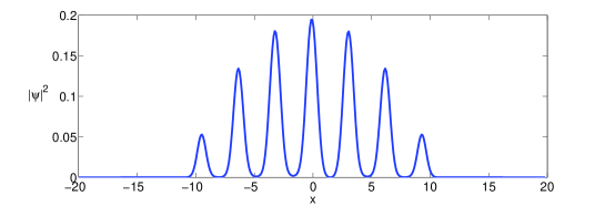
Figure 1: Solution of GP equation for a periodic one dimensional potential. It can be seen that $|\Psi|^{2}$ is enveloped by an inverted parabola shape.

Eq. 2.4 is just the Hamiltonian of a lattice of small Josephson junctions with inhomogeneous coupling constants $J_{ij}$. With $J_{ij}\gg U$, we can neglect the kinetic energy term; Moreover, we suppose that coupling constants are equal $J_{ij}=J$. This regime can be achieved when the depth of optical lattice $V_{0}$ is between 18 and 25$E_{R}$ ($E_{R}=\hbar^{2}k^{2}/2m$ is recoil energy) and average particle number is $\bar{n}\approx 170$R31 . Then we have:

$$H=-\sum_{<i,j>}cos(\gamma_{ij}),$$ (5)

with $\gamma_{ij}=\theta_{i}-\theta_{j}-A_{ij}$. Our purpose is to find minimum of this Hamiltonian as a function of condensate phases $\theta_{i}$ with two constraints as follows. First constraint originates in the single valuedness of the wave function which leads to the quantization of vorticity:

$$\sum\gamma_{ij}=2\pi(n_{k}-a_{k}f)$$ (6)

where sum is over $k$th plaquette, $a_{k}$ is area of $k$th plaquette, and $n_{k}$ is integer. In the case of a condensate with the rigid-body rotation, the frustration parameter is defined as $f=2\Omega/\kappa$ with the quantum circulation $\kappa=h/m$. In two dimensional arrays, frustration represents density of vortices per number of lattice plaquettes R44 .

The second constraint comes from conservation of the particles numbers. The particle current from the nodes can be assumed as the derivation of the energy function with respect to the corresponding phaseR43 . This leads to

$$\sum sin(\gamma_{ij})=0,$$ (7)

where sum is over all $j$ which is connected to $i$th node.

Since Hamiltonian is periodic, $n_{k}$ can be $\lfloor a_{k}f\rfloor$ or $\lfloor a_{k}f\rfloor+1$, and we can replace them by $n_{k}$ which is zero or one, and replace $a_{k}f$ with $a_{k}f-\lfloor a_{k}f\rfloor$. These two set of equations can completely determine all $\gamma_{ij}$ for a given set of $n_{k}$. Also, for a lattice, number of plaquettes plus number of nodes is equal to number of connections minus one; therefore one of the equations (e.g. one of particle conservation equations) can be neglected. Assuming the particle flow from the nodes are small, we can linearize the Eq.7 i.e. $sin{\gamma_{ij}\approx\gamma_{ij}}$. Now, we have a linear set of equations which must be solved for a given set of integers $n_{k}$, i.e. for a vortex configuration. Energy of this vortex configuration is denoted by $E_{\{n\}}$. Then instead of original minimization scheme, we can use the set of these energies for minimization of Hamiltonian. It means that minimum of Hamiltonian correspond to a vortex configuration which minimizes these set of energies, with number of vortex configuration equal to $2^{N}$ where $N$ is number of plaquettes in the lattice.

III Ladder case

In this section, we apply the formulation of previous section on a ladder geometry and find an exact analytical formula for energy of vortex configuration. It is known that a ladder geometry can give an insight about ground state vortex structure in 2D latticesR32 . As we will see the symmetry of the problem in this case, reduces the number of equations such that there will be $N$ linear algebraic equations to solve, where $N$ is number of plaquettes. One of difference between problems in Josephson junction arrays and BEC lattices is boundary condition which is imposed on lattice. In the Josephson junction arrays, the behavior of the arrays with large number of plaquettes is interestingR44 , therefore the boundary condition of lattice is usually assumed as periodic, i.e. the first plaquette is connected to the last plaquette. For BECs, the number of lattice sites is usually finite and free or fixed boundary condition are more suitable.

Conservation of current 7 imposes that current in upper and lower junctions of a plaquette and therefore their corresponding $\gamma_{ij}$ will be equal. We denote gauge invariant phase difference for upper and lower junctions of $k$th plaquette by $\gamma_{k}$ and those of the vertical junctions between $k$ and $k+1$th plaquette by $\gamma_{k,k+1}$. Then the node current equations read

$$sin(\gamma_{k,k+1})=sin(\gamma_{k})-sin(\gamma_{k+1}),$$ (8)

and the linearized approximation gives

$$\gamma_{k,k+1}=\gamma_{k}-\gamma_{k+1}.$$ (9)

Imposing this equation on the flux quantization 2.6, we have

$$4\gamma_{k}-\gamma_{k+1}-\gamma_{k-1}=2\pi(n_{k}+\lfloor a_{k}f\rfloor-a_{k}f),$$ (10)

for the $k$th plaquette with fixed boundary condition: $\gamma_{N+1}=\gamma_{0}=0$, where $N$ is number of plaquettes in ladder. We have left now with $N$ equations and $2N$ variables. Denoting coefficient matrix by $C$, we can write

$$\gamma_{k}=\sum_{k=1}^{N}C^{-1}_{kl}b_{l}=2\pi(N_{k}-A_{k}f),$$ (11)

where $b_{l}=2\pi(n_{l}-a_{l}f)$, and $C^{-1}$ is inverse of coefficient matrix and its elements are,

$$C^{-1}_{kl}=\frac{\xi^{N-|k-l|+1}+\xi^{|k-l|-N-1}-\xi^{N+1-k-l}-\xi^{k+l-N-1}}{(\xi-\xi^{-1})(\xi^{N+1}-\xi^{-N-1})},$$ (12)

where $\xi=2+\sqrt{3}$, and $A_{k}$ and $N_{k}$ are defined with appropriate summation.

By using Eq. 11 we can find the energy (normalized by the number of junctions) for a vortex configuration $\{n\}$ as:

$$E_{\{n\}} = \frac{1}{3N+1}\{\sum_{k=1}^{N}\{2cos(\gamma_{k})+cos(\gamma_{k}-\gamma_{k+1})\}$$ (13)

$$+ cos(\gamma_{N})\}.$$

Related to the problem of minimizing the Hamiltonian, each vortex configuration can be vortex configuration with minimum energy for a definite value, or an interval of $f$. Then for each value of frustration we need calculate the energy for all the vortex configurations. As an example, we begin with a square ladder ($a_{i}=1$) with $8$ plaquette in which we just need to study $0\leq f<1$. In Fig. 2 we have plotted ground state energy by the above procedure: $f$ is incremented from $0$ to $1$ by $1/128$ and for each value of $f$, energy of all the configurations is calculated and the least value has been chosen. We have specified each vortex configuration by a number $m$ which in the binary representation with $N$ digit ($N$ is number of plaquettes) gives the configuration of the vortices with every one, meaning there is vortex on that plaquette. For example $m=3$ means a vortex configuration $00000011$, i.e. there are two vortices on the $7$th and $8$th plaquettes.

Fixing $f$ we can demonstrate the dependence of the energy to the configuration of the vortices. In Fig. 3 we have plot energy vs. vortex configuration for $f=1/2$ and $2/5$ where the vortex configuration is labeled as we noted above. For $f=1/2$ we see a mirror symmetry, it means that vortex configurations $m$ and $2^{N}-m$ have the same energy. More general rule for square ladder with arbitrary $f$ can be deduced easily from above equations: vortex configuration $m$ for $f$ and $2^{N}-m$ for $1-f$ has same energy. Therefore, if vortex configuration $m$ has the minimum energy for $f$, then vortex configuration $2^{N}-m$ has the minimum energy for $1-f$. This means that for $f=1/2$, the minimum energy is twofold degenerate. For example for the ladder considered above, both $01010101$ and $10101010$ configurations give the minimum energy. In Fig. 4 we have shown position of vortices for different $f$. This figure shows that behavior of vortex is similar to the behavior of a charge $q$ on a lattice with opposite sign onsite chargesR44 ; R45 . When we have one vortex on lattice, the vortex prefers to sit on middle of ladder, where in this case it can be two plaquettes 4 or 5. When we have two vortices on ladder, they prefer to divide ladder into three equal parts, which means that they must be on plaquettes 3 and 6. This description can be applied to vortex configurations with more vortices.

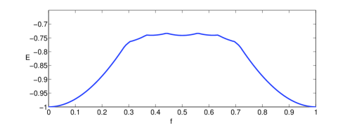
Figure 2: Ground state energy of a square lattice with 8 plaquettes. For each value of $f$, energy of all vortex configurations is calculated and the smallest value has been chosen.

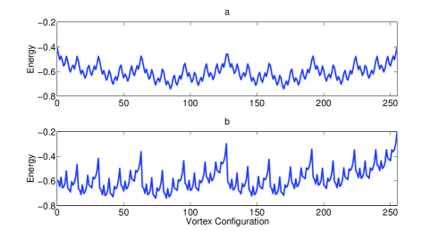
Figure 3: Energy of vortex configurations for square ladder with 8 plaquettes. Binary representation is used to demonstrate vortex configurations as is explained in the text. $f=1/2$ in (a) and $f=2/5$ in (b).

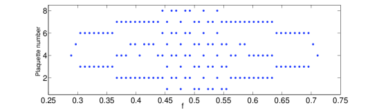
Figure 4: Position of vortex for a square ladder with 8 plaquettes. Vertical axis shows the position of plaquette in the array.

For more accurate results, we can relax linear approximation for the current equation and use Newton-Raphson method, with the initial estimation from linear approximation. For above case, we compare linear approximation and 10 iterates of Newton-Raphson method in Fig. 5. It worth to mention while energy differences are small but, in some small intervals of $f$, different vortex configurations give the minimum energy.

IV MC formulation for vortex configuration

When $N$ number of plaquettes grows, number of possible vortex configurations grows as $2^{N}$, and expect for small number of plaquettes we can not determine the exact minimum vortex configuration which needs checking all of vortex configuration. Therefore we use a Monte-Carlo method: we start from a high temperature $T$ and a random vortex lattice $n$ and calculate its energy $E_{n}$. Then we decrease temperature gradually and for each temperature we do following process a few times: we change the configuration randomly to $n^{\prime}$ with energy $E_{n^{\prime}}$, we accept the new configuration if $exp(-\Delta E/T)<r$ where $r$ is a random number between $0$ and $1$, and $\Delta E=E_{n}-E_{n^{\prime}}$. When temperature receives $0.0001$, we take the final configuration as ground state.

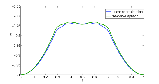
Figure 5: Comparison between linear approximation (blue) and the Newton-Raphson method (green).

For a periodic lattice finding the ground state from the MC method is troublesome for nonzero frustrationR47 . To check the validity of our method, instead, we apply the method on a quasiperiodic lattice e.g. a Fibonacci ladder. The Fibonacci ladders contains two types of plaquettes with lengths 1 and $\tau=(1+\sqrt{(}5))/2$. If we denote plaquette with length 1 and $\sigma$, by $S$ and $L$ respectively, then these two types of plaquettes arranged in bases of the following rule: for $(n+1)$th step of construction, we add $(n-1)$th step to end of $n$th step. With first step $S$ and second step $L$, we have: $LS,LSL,LSLLS,LSLLSLSL,...$. The results are shown in Fig. 6 along with the result of using the Monte-Carlo on the original Hamiltonian, with a good agreement (we note that for a aperiodic lattice it is not sufficient to study $0\leq f<1$). For a square lattice, increasing $f$ from $0$ to $1/2$, both the number of the vortices and the magnitude of vorticity grow R44 and the linear approximation may seem unreasonable. Fig. 6 shows that despite this fact, the approximate results are in a good agreement with the results of the direct method.

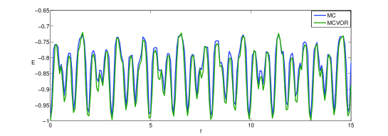
Figure 6: Comparison between energy obtained by the direct Monte-Carlo method (MC) and by the Monte-Carlo method with vortex configuration formulation (MCVOR).

V Conclusion

The configuration of the vortex lattice of rotating BECs in an Optical lattice is investigated. For deep Optical Lattices when the number of particles in each site is large, the problem of rotating BEC in an optical lattice, can be mapped onto the model of arrays of Josephson junctions in presence of an external magnetic field. In this approximation we have formulated a vortex configuration for the ground state. Our result for ladder case is presented and is in good agreement with Monte-Carlo result with original JJA Hamiltonian. This method can be extended to 2D case, and also cases with non-uniform coupling which looks more relevant for study of rotating BECs. In these cases, with linear approximation, we deal with a set of linear algebraic equations for each vortex configuration which can be solved easily by use of proposed method.

Effect of non-uniform coupling can affect the results especially in the situation of high density of vortices as in the case $f=1/2$ for square lattice. Also as a better approximation we can consider finite $U$, then problem is similar to the arrays of small Josephson junctionsR37 ; R38 ; R39 . We can also suppose that coupling is time-dependent which can occur in case of a vibrating optical latticeR46 . Then problem can be treated as a set of coupled pendulum equations with time-dependent lengthsR1 .

References

- (1) M. H. Anderson, J. R. Ensher, M. R. Mathews, C. E. Wieman, and E. A. Cornell, Scinece 269, 198 (1995).
- (2) C. J. Pethick and H. Smith, Bose-Einstein Condensation in Dilute Gases, Cambridge University Press (2001).
- (3) J. O. Andersed, Rev. Mod. Phys. 76, 599 (2004).
- (4) O. Morsch and M. Oberthaler, Rev. Mod. Phys. 78, 179 (2006).
- (5) I. Bloch, Nature Phys. 1, 23 (2005).
- (6) M. Ben Dahan, E. Peik, J. Reichel, Y. Castin, and C. Salomon, Phys. Rev. Lett. 76, 4508 (1996).
- (7) E. Peik, M. Ben Dahan, I. Bouchoule, Y. Castin, and C. Salomon, Phys. Rev. A 55, 2989 (1997).
- (8) O. Morsch, J. H. Muller, M. Cristiani, D. Ciampini, and E. Arimondo, Phys. Rev. Lett. 87, 140402 (2001).
- (9) M. Cristiani, O. Morsch, J. H. Muller, D. Ciampini, and E. Arimondo, Phys. Rev. A 65, 063612 (2002).
- (10) S. R. Wilkinson, C. Bharucha, K. W. Madison, Q. Niu, and M. G. Raizen, Phys. Rev. Lett. 76, 4512 (1996).
- (11) F. S. Cataliotti, S. Burger, C. Fort, P. Maddaloni, F. Minardi, A. Trambettoni, A. Smerzi, and M. Inguscio, Science 293, 843 (2001).
- (12) K. Kasamatsu, J. Low Temp. Phys. 150, 593 (2008).
- (13) B. P. Anderson and M. A. Kasevich, Science 282, 1686 (1998).
- (14) K. Kasamatsu, Phys. Rev. A 79, 021604(R) (2009).
- (15) S. Levy, E. Lahoud, I. Shomroni, and J. Steinhauer, Nature 449, 579 (2007).
- (16) M. Polini, R. Fazio, M. P. Tosi, J. Sinova, and A. H. MacDonald, Laser Phys. 14, 603 (2004).
- (17) M. Polini, R. Fazio, A. H. MacDonald, and M. P. Tosi, Phys. Rev. Lett. 95, 010401 (2005).
- (18) D. Jaksch, C. Burder, J. I. Cirac, C. W. Gardiner, and P. Zoller, Phys. Rev. Lett. 81, 3108 (1998).
- (19) M. Griener, O. Mandel, T. Esslinger, T. W. Hansch, and I. Bloch, Nature (London) 415, 39 (2002).
- (20) Y. Fujihara, A. Koga, and N, Kawakami,Phys. Rev. A 79, 0131610 (2009).
- (21) T. Giamarchi, C. Ruegg, and O. Tchernyshyov, Nature Phys. 4, 198 (2008).
- (22) H. Zhai, R. O. Umucahlar, and M. O. Oktel, Phys. Rev. Lett. 104, 145301 (2010).
- (23) K. W. Madison, E. Chevy, V, Bretin, and J. Dalibard, Phys. Rev. Lett. 86, 4443 (2001).
- (24) N. R. Cooper, Advanced in Physics 57, 539 (2008).
- (25) A. L. Fetter, Rev. Mod. Phys. 81, 647 (2009).
- (26) G. Watanabe, S. A. Gafford, G. Bayam, and C. J. Pethik, Phys. Rev. A 74, 063621 (2006).
- (27) N. R. Cooper, S. Komineas, and N. Read, Phys. Rev. A 70, 033604 (2004).
- (28) A. Aftalio, X. Blanc, and J. Dalibard, Phys. Rev. A 71, 023611 (2005).
- (29) S. I. Matreenko, D. Kovrizhin, S. Ouvry, and G. V. Shlyapnikov, arXiv:0908.2172v2 [cond-mat.quant-gas] (2009).
- (30) S. Tung, V. Schweikhard, and E. A. Cornell, Phys. Rev. Lett. 97, 240402 (2006).
- (31) V. Schwiekhard, S. Tung, and E. A. Cornell, Phys. Rev. Lett. 99, 030401 (2007).
- (32) J. Zhang, C. M. Jian, F. Ye, and H. Zhai, Phys. Rev. Lett. 105, 155302 (2010).
- (33) L. Sanchez-Palencia and L. Santos, Phys. Rev. A 72, 053607 (2005).
- (34) L. Gaindini, C. Triche, P. Verkerk, and G. Grynberg, Phys. Rev. Lett. 79, 3363 (1997).
- (35) G. Grynberg and C. Robilliard, Phys. Rep. 355, 335 (2000).
- (36) R. B. Diener, G. A. Georgakis, J. Zhang, M. Raizen, and Q. Niu, Phys. Rev. A 64, 033416 (2001).
- (37) T. C. Halsey, Phys. Rev. B 31, 5728 (1985).
- (38) M. R. Kolahchi and J. P. Straley, Phys. Rev. B 66, 144502 (2002).
- (39) G. Grynberg, B. Lounis, P. Verkerk, J. Y. Courtois, and C. Salomon, Phys. Rev. Lett. 70, 2249 (1993).
- (40) J. E. Lye, L. Fallani, M. Modugno, D. S. Wiersma, C. Fort, and M. Inguscio, Phys. Rev. Lett. 95, 070401 (2005).
- (41) A. Trombettoni, A. Smerzi, and P. Sodano, New. J. Phys. 7, 57 (2005).
- (42) S. Teitel and C. Jayaprakash, Phys. Rev. Lett. 51, 1999 (1983).
- (43) F. Meier and W. Zwerger, Phys. Rev. A 64, 033610 (2001).
- (44) E. Fradkin, B. A. Huberman, S. H. Shenker, Phys. Rev. B 18, 4789 (1978).
- (45) J. P. Straley and G. M. Barnett, Phys. Rev. B 48, 3309 (1993).
- (46) C. D. Chen, P. Delsiny, D. B. Haviland, Y. Harda, and T. Claeson, Phys. Rev. B 54, 9449 (1996).
- (47) W. Zwerger, Phys. Rev. B 35, 4737 (1987).
- (48) Y. Takahide, R. Yagi, A. Kanda, Y. Ootulca, and S. Kobyashi, Phys. Rev. Lett. 85, 1974 (2000).
- (49) Y. B. Band and M. Trippenbach, Phys. Rev. A 65, 053602 (2002).