Three-Dimensional Lattice Boltzmann Model for High-Speed Compressible Flows

Abstract

A highly efficient three-dimensional (3D) Lattice Boltzmann (LB) model for high speed compressible flows is proposed. This model is developed from the original one by Kataoka and Tsutahara[Phys. Rev. E 69, 056702 (2004)]. The convection term is discretized by the Non-oscillatory, containing No free parameters and Dissipative (NND) scheme, which effectively damps oscillations at discontinuities. To be more consistent with the kinetic theory of viscosity and to further improve the numerical stability, an additional dissipation term is introduced. Model parameters are chosen in such a way that the von Neumann stability criterion is satisfied. The new model is validated by well-known benchmarks, (i) Riemann problems, including the problem with Lax shock tube and a newly designed shock tube problem with high Mach number; (ii) reaction of shock wave on droplet or bubble. Good agreements are obtained between LB results and exact ones or previously reported solutions. The model is capable of simulating flows from subsonic to supersonic and capturing jumps resulted from shock waves.

I Introduction

Lattice Boltzmann (LB) method has been becoming a powerful and efficient tool to simulate fluid flows in many areas 1 , ranging from multiphase flows 2 ; 3 , magnetohydrodynamics 4 ; 5 ; 6 , flows through porous media 7 ; 8 and thermal fluid dynamics 9 . However, most models so far work only for incompressible fluids. Many attempts have been made in constructing LB models for the compressible Euler equations. Hu et al. 10 proposed a 13-discrete-velocity model based on the triangular lattice. In this model, particles at each node are classified into three kinds. They are on the energy levels $\epsilon_{A}$, $\epsilon_{B}$, and $\epsilon_{D}$, where $\epsilon_{A}>\epsilon_{B}>0$, the energy level $\epsilon_{D}$ is higher than $0$ and is for the rest particle. Similar to Hu’s model, Yan and co-workers 11 presented a 17-discrete-velocity model with three-speed-three-energy level on a square lattice. Both models are two-dimensional (2D) and belong to the standard LB model. In the standard LB model, particle velocities are restricted to those exactly linking the lattice nodes in unit time. Besides the standard LB, Finite Difference (FD) LB is attracting more attention with time. With the FD LB model we do not need consider that constraint, we can choose particle velocities independently from the lattice configuration.

Shi et al. 12 formulated a FD LB scheme based on a two-dimensional 9-velocity model. This model allows particles to possess both kinetic and thermal energies. Kataoka and Tsutahara 13 presented a LB model series for the compressible Euler equations, where 5, 9 and 15 discrete velocities are used for the one- , two- and three-dimensional cases, respectively. However, all these models work only for subsonic flow. The low-Mach number constraint is generally related to the numerical stability problem. The latter has been partly addressed by a few potential solutions, for example, the entropic method entropic , flux limiters Sofonea , dissipation techniques 16 ; gan ; chen ; Brownlee and multiple-relaxation-time LB approach EPLChen .

Watari and Tsutahara proposed a three-dimensional FD LB model for Euler equations, where numerical simulations are successfully performed up to Mach number 1.7 14 . But the number of discrete velocities in that model is up to 73, which is quite expensive from the view of computational side. Recently, a three-dimensional compressible FD LB model without free parameters was proposed 15 , where 25 discrete velocities are used. With this model the momentum equations at the Navier-Stokes level and energy equation at the Euler level can be recovered. The maximum Mach number is 2.9 in simulations. Pan, et al. 16 developed the 2D model by Kataoka and Tsutahara 13 by introducing reasonable dissipation term so that the model works for supersonic flows. Flows with Mach number higher than 30 are successfully simulated with the model.

In this paper we formulate a three-dimensional FD LB model for high speed compressible flows, based on Kataoka’s 15-velocity model and reasonable dissipation technique. The following part of the paper is planned as follows. Section 2 presents the discrete velocity model used in this work. Section 3 describes briefly the FD scheme and performs the von Neumann stability analysis. Simulation results are presented and analyzed in Section 4. Section 5 makes the conclusion.

II 3D Discrete Velocity Model by Kataoka and Tsutahara

The evolution of the distribution function $f_{i}$ is governed by the following equation 17 :

$$\frac{\partial f_{i}}{\partial t}+v_{i\alpha}\ \frac{\partial f_{i}}{\partial x_{\alpha}}=-\frac{1}{\tau}\left[f_{i}-f_{i}^{eq}\right],$$ (1)

where $v_{i\alpha}$ is the $\alpha$ component of velocity $v_{i}$, $i=1,\ldots,N$, $N$ is the number of discrete velocities, index $\alpha=1$, $2$, $3$ corresponding to $x$, $y$, and $z$, respectively. The Einstein’s convention for sums is used. The variable $t$ is time, $x_{\alpha}$ is the spatial coordinate, $f_{i}^{eq}$ is the local-equilibrium distribution function, and $\tau$ represents the relaxation time. At the continuous limit, the above formulation is required to recover the following Euler equations:

$$\frac{\partial\rho}{\partial t}+\frac{\partial(\rho u_{\alpha})}{\partial x_{\alpha}} = 0,$$

$$\frac{\partial(\rho u_{\alpha})}{\partial t}+\frac{\partial(\rho u_{\alpha}u_{\beta})}{\partial x_{\beta}}+\frac{\partial P}{\partial x_{\alpha}} = 0,$$ (2)

$$\frac{\partial\rho(bRT+u_{\alpha}^{2})}{\partial t}+\frac{\partial\rho u_{\alpha}(bRT+u_{\beta}^{2})+2Pu_{\alpha}}{\partial x_{\beta}} = 0\text{,}$$

where $\rho$, $u_{\alpha}$, $T$, $P$ are, respectively, the density, the flow velocity in the $x_{\alpha}$ direction, the temperature, and the pressure of gas. $R$ is the specific gas constant and $b$ is a constant relating to the specific-heat ratio $\gamma$, $b=2/(\gamma-1)$. The 3D discrete velocity model proposed by Kataoka and Tsutahara (see Fig. 1) can be expressed as:

$$\left(v_{i1},v_{i2},v_{i3}\right)=\left\{\begin{array}[]{cc}\left(0,0,0\right)&\text{for }i=1,\\ c_{1}\left(\pm 1,0,0\right),c_{1}\left(0,\pm 1,0\right),c_{1}\left(0,0,\pm 1\right)&\text{for }i=2,3,\cdots,7,\\ \frac{c_{2}}{\sqrt{3}}\left(\pm 1,\pm 1,\pm 1\right)&\text{for }i=8,9,\cdots,15,\end{array}\right.$$

$$\eta_{i}=\left\{\begin{array}[]{cc}\eta_{0},&\text{for }i=1,\\ 0,&\text{for }i=2,3,\cdots,15,\end{array}\right.$$ (3)

where $c_{1}$,$c_{2}$, and $\eta_{0}$ are given nonzero constants.

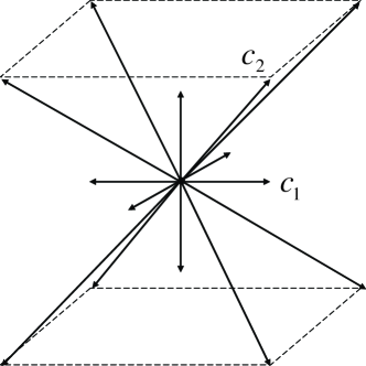
Figure 1: Distribution of $\mathbf{v}_{i}$ for the proposed discrete velocity model.

In this model, the local-equilibrium distribution function $f_{i}^{eq}$ satisfies the following relations:

$$\rho=\sum_{i=1}^{N}f_{i}^{eq}\text{,}$$ (4a)

$$\rho u_{\alpha}=\sum_{i=1}^{N}f_{i}^{eq}v_{i\alpha}\text{,}$$ (4b)

$$\rho(bRT+u_{\alpha}^{2})=\sum_{i=1}^{N}f_{i}^{eq}(v_{i\alpha}^{2}+\eta_{i}^{2})\text{,}$$ (4c)

$$P\delta_{\alpha\beta}+\rho u_{\alpha}u_{\beta}=\sum_{i=1}^{N}f_{i}^{eq}v_{i\alpha}v_{i\beta}\text{,}$$ (4d)

$$\rho[(b+2)RT+u_{\beta}^{2}]u_{\alpha}=\sum_{i=1}^{N}f_{i}^{eq}(v_{i\alpha}^{2}+\eta_{i}^{2})v_{i\alpha}\text{.}$$ (4e)

The local-equilibrium distribution function  $$f_{i}^{eq}$$ is defined as follows:

$$f_{i}^{eq}=\rho(A_{i}+B_{i}v_{i\alpha}u_{\alpha}+D_{i}u_{\alpha}v_{i\alpha}u_{\beta}v_{i\beta})\text{, }i=1,2,...,15\text{,}$$ (5)

where

$$A_{i}=\left\{\begin{array}[]{ll}\frac{b-3}{\eta_{0}^{2}}T\text{,}&\text{ }i=1\\ \frac{1}{6(c_{1}^{2}-c_{2}^{2})}\left[-c_{2}^{2}+\left((b-3)\frac{c_{2}^{2}}{\eta_{0}^{2}}+3\right)T+\frac{c_{2}^{2}}{c_{1}^{2}}u_{\alpha}^{2}\right]\text{, }&i=2,3,\cdots,7\\ \frac{1}{8(c_{2}^{2}-c_{1}^{2})}\left[-c_{1}^{2}+\left((b-3)\frac{c_{1}^{2}}{\eta_{0}^{2}}+3\right)T+\frac{3c_{1}^{2}-c_{2}^{2}}{2c_{2}^{2}}u_{\alpha}^{2}\right]\text{,}&\text{ }i=8,9,\cdots,15\end{array}\right.$$

$$B_{i}=\left\{\begin{array}[]{ll}0,&i=1\\ \frac{-c_{2}^{2}+(b+2)T+u_{\beta}^{2}}{2c_{1}^{2}(c_{1}^{2}-c_{2}^{2})},&i=2,3,\cdots,7\\ \frac{3[-c_{1}^{2}+(b+2)T+u_{\beta}^{2}]}{8c_{2}^{2}(c_{2}^{2}-c_{1}^{2})},&\text{ }i=8,9,\cdots,15\end{array}\right.\text{, }D_{i}=\left\{\begin{array}[]{cc}0,&i=1\\ \frac{1}{2c_{1}^{4}},&i=2,3,\cdots,7\\ \frac{9}{16c_{2}^{4}},&i=8,9,\cdots,15\end{array}\right.$$ (6)

III FD Scheme and Von Neumann Stability Analysis

In the original LB model 13 , the finite difference scheme with the first-order forward in time and the second-order upwind in space is used for the numerical computation. This model has been validated via the Riemann problem in subsonic flows and encounters instability problems in supersonic flows. In order to improve the stability, we adopt the Non-oscillatory, containing No free parameters and Dissipative (NND) scheme for space discretization. To be more consistent with the kinetic theory of viscosity and to further improve the numerical stability, an additional dissipation term is introduced.

In the NND scheme, the spacial derivative is calculated using the following formula:

$$\frac{\partial\left(v_{i\alpha}f_{i}\right)}{\partial x_{\alpha}}=\frac{1}{\triangle x_{\alpha}}\left(h_{i,I+\frac{1}{2}}-h_{i,I-\frac{1}{2}}\right),$$ (7)

where $I$ represents node index in $x$ or $y$ direction. $h_{i,I+\frac{1}{2}}$ is the numerical flux at the interface of $\left(x_{I}+\frac{\Delta x}{2},y\right)$ or $\left(x,y_{I}+\frac{\Delta y}{2}\right)$, and defined as:

$$h_{i,I+\frac{1}{2}}=f_{i,I+\frac{1}{2}}^{L}+f_{i,I+\frac{1}{2}}^{R},$$ (8)

where

$$f_{i,I+\frac{1}{2}}^{L}=f_{i,I}^{+}+\frac{1}{2}\min\mathtt{mod}\left(\Delta f_{i,I+\frac{1}{2}}^{+},\Delta f_{i,I-\frac{1}{2}}^{+}\right)\text{,}$$

$$f_{i,I+\frac{1}{2}}^{R}=f_{i,I+1}^{-}-\frac{1}{2}\min\mathtt{mod}\left(\Delta f_{i,I+\frac{1}{2}}^{-},\Delta f_{i,I+\frac{3}{2}}^{-}\right)\text{,}$$

$$f_{i,I}^{+}=\frac{1}{2}\left(v_{i\alpha}+\left|v_{i\alpha}\right|\right)f_{i,I},f_{i,I}^{-}=\frac{1}{2}\left(v_{i\alpha}-\left|v_{i\alpha}\right|\right)f_{i,I}\text{,}$$

$$\Delta f_{i,I+\frac{1}{2}}^{\pm}=f_{i,I+1}^{\pm}-f_{i,I}^{\pm}\text{,}$$

$$\min\mathtt{mod}\left(X,Y\right)=\frac{1}{2}\min\left(\left|X\right|,\left|Y\right|\right)\left[\mathtt{Sign}\left(X\right)+\mathtt{Sign}\left(Y\right)\right]\text{.}$$ (9)

The NND scheme itself contains a forth-order dissipation term with a negative coefficient which reduces the oscillations, but it is not enough to highly improve the stability, which means an additional dissipation term is needed for a practical LB simulation. In order to further improve the stability, and enhance its applicability for high Mach flows, we introduce artificial viscosity into the LB equation:

$$\frac{\partial f_{i}}{\partial t}+v_{i\alpha}\frac{\partial f_{i}}{\partial x_{\alpha}} = -\frac{1}{\tau}\left(f_{i}-f_{i}^{eq}\right)+\lambda_{i}\sum_{\alpha=1}^{3}\frac{\partial^{2}f_{i}}{\partial x_{\alpha}^{2}},$$ (10)

where

$$\lambda_{i}=\left\{\begin{array}[]{ll}c_{1}\Delta x,&i=1\\ c_{1}\Delta x/10,&i=2,3,\cdots,7\\ 0,&i=8,9,\cdots,15\end{array}\right.\text{.}$$

The second-order derivative can be calculated by the central difference scheme.

In the following we do the von Neumann stability analysis of the improved LB model. In the stability analysis, we write the solution of FD LB equation in Fourier series form. If all the eigenvalues of the coefficient matrix are less than 1, the algorithm is stable.

Distribution function is split into two parts: $f_{i}(x_{\alpha},t)=\bar{f_{i}^{0}}+\Delta f_{i}(x_{\alpha},t)$, where $\bar{f_{i}^{0}}$ is the global equilibrium distribution function. It is a constant which does not change with time or space. Putting this equation into Eq. (10) we obtain:

$$\frac{\Delta f_{i}(x_{\alpha},t+\Delta t)-\Delta f_{i}(x_{\alpha},t)}{\Delta t}+v_{i\alpha}\frac{\partial f_{i}}{\partial x_{\alpha}}=-\frac{1}{\tau}\left(\Delta f_{i}-\Delta f_{i}^{eq}\right)+\lambda_{i}\frac{\partial^{2}f_{i}}{\partial x_{\alpha}^{2}}\text{,}$$ (11)

the solution can be written as

$$\Delta f_{i}(x_{\alpha},t)=F_{i}^{t}\mathrm{exp}(\mathbf{i}k_{\alpha}x_{\alpha}),$$ (12)

where $F_{i}^{t}$ is an amplitude of sine wave at lattice point $x_{\alpha}$ and time $t$, $k_{\alpha}$ is the wave number. From the Eq.(11) and Eq.(12) we can get $F_{i}^{t+\Delta t}=G_{ij}F_{j}^{t}.$ Coefficient matrix $G_{ij}$ describes the growth rate of amplitude $F_{i}^{t}$ in each time step $\Delta t$. The von Neumann stability condition is $\mathrm{max}|\omega|\leq 1$, where $\omega$ denotes the eigenvalue of coefficient matrix. Coefficient matrix $G_{ij}$ of NND scheme can be expressed as follows,

$$G_{ij} =\left(1-\frac{\Delta t}{\tau}-\frac{v_{i\alpha}\Delta t}{\Delta x_{\alpha}}\phi\right)\delta_{ij}+\frac{\Delta t}{\tau}\frac{\partial f_{i}^{eq}}{\partial f_{j}}+\lambda_{i}\Delta t\frac{(e^{\mathbf{i}k_{\alpha}\Delta x_{\alpha}}-2+e^{-\mathbf{i}k_{\alpha}\Delta x_{\alpha}})}{(\Delta x_{\alpha})^{2}}\delta_{ij},$$

$$\phi=\left\{\begin{array}[]{ll}\left(1-\widetilde{\alpha}\right)\left(1-e^{-\mathbf{i}k_{\alpha}\Delta x_{\alpha}}\right),&\text{if }v_{i\alpha}\geq 0\text{;}\\ \left(1-\widetilde{\beta}\right)\left(e^{\mathbf{i}k_{\alpha}\Delta x_{\alpha}}-1\right),&\text{if }v_{i\alpha}<0\text{.}\end{array}\right.$$

$$\frac{\partial f_{i}^{eq}}{\partial f_{j}}=\frac{\partial f_{i}^{eq}}{\partial\rho}\frac{\partial\rho}{\partial f_{j}}+\frac{\partial f_{i}^{eq}}{\partial T}\frac{\partial T}{\partial f_{j}}+\frac{\partial f_{i}^{eq}}{\partial u_{\alpha}}\frac{\partial u_{\alpha}}{\partial f_{j}}\text{,}\left|\widetilde{\alpha}\right|<\frac{1}{2},\left|\widetilde{\beta}\right|<\frac{1}{2}\text{.}$$ (13)

There are some numerical results of von Neumann stability analysis by Mathematica. Abscissa is $kdx$, and ordinate is $|\omega|_{max}$ that is the biggest eigenvalue of coefficient matrix $G_{ij}$.

Figure 2 shows the stability analysis of several finite difference schemes. The macroscopic variables are set as $(\rho,u_{1},u_{2},u_{3},T)$ = $(1.0,4.0,0.0,0.0,1.0)$, the other model parameters are: $(c_{1},c_{2},\eta_{0})$ = $(4.0,12.0,4.0)$, $dx=dy=dz=4\times 10^{-3}$, $dt=\tau=10^{-5}$, $b=5$, $\widetilde{\alpha}=\widetilde{\beta}=0$. In this test, the NND scheme shows better stability than the others. Figure 3 shows the effect of dissipation term. The variables are set as $(\rho,u_{1},u_{2},u_{3},T)$ = $(1.0,20.0,0.0,0.0,1.0)$, $(c_{1},c_{2},\eta_{0})$ = $(20.0,60.0,20.0)$, and the others are consistent with the Figure 2. In the two cases of Figure 3, operation with dissipation term is more stable($\mathrm{max}|\omega|\leq 1$).

Figure 4 shows the influence of parameters $c_{1}$, $c_{2}$, $\eta_{0}$ on the stability in the absence of dissipation term. The macroscopic variables and the other model parameters are consistent with those of Figure 2. Figure 5 shows the stability effect of the three parameters, when there is a dissipation term. The macroscopic variables and the other model parameters are consistent with those of Figure 3. In Figure 4 constants $c_{1}$, $c_{2}$ and $\eta_{0}$ affect the stability heavily. In Figure 5 the LB is stable for all tested values of $c_{2}$ and $\eta_{0}$. Based on these tests, we suggest that $c_{1}$ can be set a value close to the maximum of flow velocity, $c_{2}$ can be chosen about $3$ times of the value of $c_{1}$, and $\eta_{0}$ can be set to be about $1\sim 2$ times of the value of $c_{1}$.

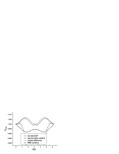
Figure 2: Stability analysis of several finite difference schemes.

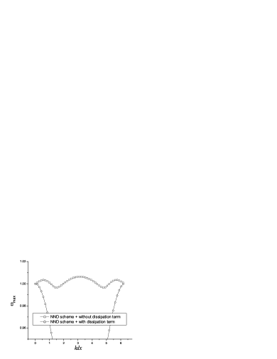
Figure 3: Effect of dissipation term on numerical stability.

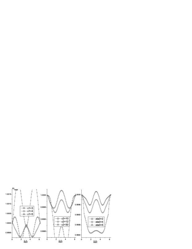
Figure 4: Influence of parameters $c_{1}$, $c_{2}$, $\eta_{0}$ on stability in the absence of artificial viscosity.

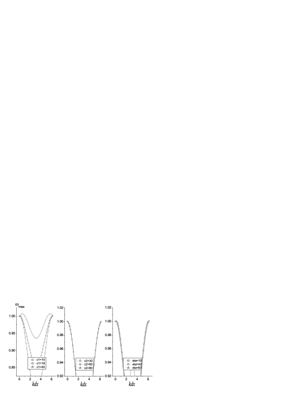
Figure 5: Effect of $c_{1}$, $c_{2}$, $\eta_{0}$ under the condition with artificial viscosity term.

IV Numerical Simulation and Analysis

In this section we study the following questions using the proposed LB model: one-dimensional Riemann problems, and reaction of shock wave on a droplet or bubble.

(1)One-dimensional Riemann problems

Here, we study two one-dimensional Riemann problems, including the problem with Lax shock tube and a newly designed shock tube problem with high Mach number. Subscripts “L” and “R” indicate the left and right macroscopic variables of discontinuity.

(a) Lax shock tube problem

The initial condition of the problem can be defined:

$$\begin{array}[]{cc}(\rho,u_{1},u_{2},u_{3},T)|_{L}=(0.445,0.698,0.0,0.0,7.928),\\ (\rho,u_{1},u_{2},u_{3},T)|_{R}=(0.5,0.0,0.0,0.0,1.142).\end{array}$$ (14)

Figure 6 shows the comparison of the NND scheme and the second-order upwind scheme without the dissipation term at $t=0.1$. Circles are for the NND scheme simulation results, squares correspond with the second-order upwind scheme, and solid lines are for exact solutions. The parameters are $(c_{1},c_{2},\eta_{0})$ = $(2.0,6.0,2.0)$, $\gamma=1.4$, $dx=dy=dz=0.003$, $dt=\tau=10^{-5}$. Compared with the simulation results of second-order upwind scheme, the oscillations at the discontinuity are weaker in the NND simulation.

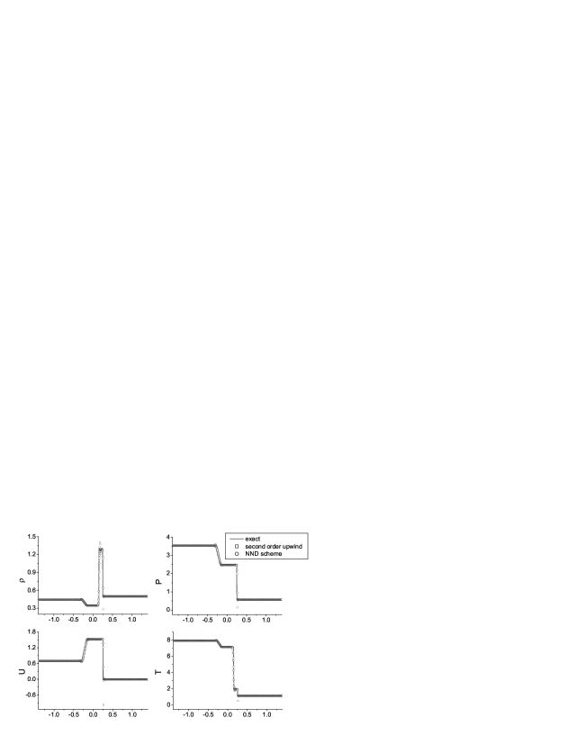
Figure 6: Numerical results and exact solutions for Lax shock tube at $t=0.1$.

(b) High Mach number shock tube problem

In order to test the Mach number of the new model, we construct a new shock tube problem with high Mach number, and the initial condition is

$$\begin{array}[]{cc}(\rho,u_{1},u_{2},u_{3},T)|_{L}=(100.0,10.0,0.0,0.0,0.714286),\\ (\rho,u_{1},u_{2},u_{3},T)|_{R}=(150.0,0.0,0.0,0.0,50.0).\end{array}$$ (15)

Figure 7 shows a comparison of the numerical results and exact solutions at $t=0.25$, where $(c_{1},c_{2},\eta_{0})$ = $(8.0,24.0,8.0)$, $\gamma=1.4$, $dx=dy=dz=0.01$, $dt=\tau=10^{-5}$. The Mach number of the left side is $10$ ($Ma=u/\sqrt{\gamma T}=10/\sqrt{1.4\times 0.714286}$), and the right is $0$ ($Ma=u/\sqrt{\gamma T}=0$). Successful simulation of this test shows the proposed model is still likely to have a high stability when the Mach number is large enough.

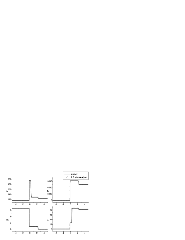
Figure 7: The numerical and exact solutions for high Mach number shock tube at $t=0.25$.

(2) Reaction of shock wave on 3D bubble problem

The proposed model is used to simulate interaction of a planar shock wave with a bubble or droplet. The shock wave is moving from the right to the left. Initial conditions are (a)

$$\left(\rho,u_{1},u_{2},u_{3},p\right)\mid_{x\text{,}y\text{,}0}=\left\{\begin{array}[]{cc}\left(1,0,0,0,1\right),&\mathbf{pre-shock,}\\ \left(2.66667,-1.47902,0,0,3.94406\right),&\mathbf{post-shock,}\\ \left(0.1358,0,0,0,1\right),&\mathbf{bubble,}\end{array}\right.$$ (16)

and (b)

$$\left(\rho,u_{1},u_{2},u_{3},p\right)\mid_{x\text{,}y\text{,}0}=\left\{\begin{array}[]{cc}\left(1,0,0,0,1\right),&\mathbf{pre-shock,}\\ \left(2.66667,-1.47902,0,0,3.94406\right),&\mathbf{post-shock,}\\ \left(4.1538,0,0,0,1\right),&\mathbf{bubble.}\end{array}\right.$$ (17)

The corresponding shock wave Mach number is $2.0$, ($Ma=(D-u)/\sqrt{\gamma T}=(2.36643-0)/\sqrt{1.4\times 1}$, where $D=2.36643$ is the wavefront velocity).

The domain of computation is $(0:301,0:81,0:81)$. Initially, the bubble or droplet is at the position (200,40,40). In the simulations, the right side adopts the values of the initial post-shock flow, the extrapolation technique is applied at the left boundary, and reflection conditions are imposed on the other four surfaces. Specifically, at the right side,

$$\begin{array}[]{c}\rho(NX+1,iy,iz)=\rho(NX,iy,iz)=2.66667\text{,}\\ T(NX+1,iy,iz)=T(NX,iy,iz)=1.6875\text{,}\\ u_{1}(NX+1,iy,iz)=u_{1}(NX,iy,iz)=-1.47902\text{,}\\ u_{2}(NX+1,iy,iz)=u_{2}(NX,iy,iz)=0\text{,}\\ u_{3}(NX+1,iy,iz)=u_{3}(NX,iy,iz)=0\text{,}\end{array}$$

where $ix$ (or $iy$, $iz$) is the index of lattice node in the $x$- (or $y$-, $z$-) direction, and $ix=0$, $1$, $\cdots$, $NX+1$ ( $iy=0$, $1$, $\cdots$, $NY+1$; $iz=0$, $1$, $\cdots$, $NZ+1$). At the left side $\rho(1,iy,iz)=2\rho(2,iy,iz)-\rho(3,iy,iz)\text{, }\rho(0,iy,iz)=2\rho(1,iy,iz)-\rho(2,iy,iz)$, temperature and velocity components have the same form. Finally we take the upper surface as an example to describe the reflection conditions.

$$\rho(ix,NY+1,iz) = \rho(ix,NY-1,iz)\text{,}$$

$$T(ix,NY+1,iz) = T(ix,NY-1,iz)\text{,}$$

$$u_{1}(ix,NY+1,iz) = u_{1}(ix,NY-1,iz)\text{,}$$

$$u_{2}(ix,NY+1,iz) = -u_{2}(ix,NY-1,iz)\text{,}$$

$$u_{3}(ix,NY+1,iz) = u_{3}(ix,NY-1,iz)\text{,}$$

$$\rho(ix,NY,iz) = \rho(ix,NY-1,iz)\text{,}$$

$$T(ix,NY,iz) = T(ix,NY-1,iz)\text{,}$$

$$u_{1}(ix,NY,iz) = u_{1}(ix,NY-1,iz)\text{,}$$

$$u_{2}(ix,NY,iz) = 0\text{,}$$

$$u_{3}(ix,NY,iz) = u_{3}(ix,NY-1,iz)\text{.}$$

Parameters are as follows: $(c_{1},c_{2},\eta_{0})$ = $(2.0,6.0,4.0)$, $\gamma=1.4$, $dx=dy=dz=0.001$, $dt=\tau=10^{-5}$. Figure 8 and Figure 9 show the density iso-surfaces of bubble or droplet, where Figure 8 is for the process with initial condition (16), and Figure 9 is for condition (17). Figure 10 shows the density contours on section $z=40$, where (a) and (b) correspond to the processes of Figure 8 and Figure 9, respectively. The simulation results are accordant with those by other numerical methods18 ; 19 and experiment20 .

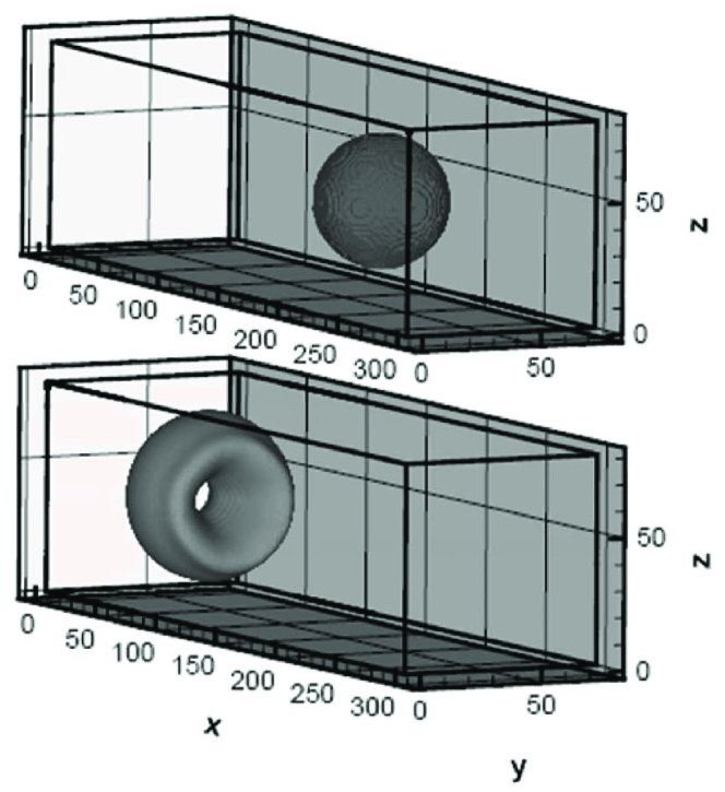
Figure 8: Density iso-surfaces of a low density bubble at $t=0.0$, $0.1$, respectively.

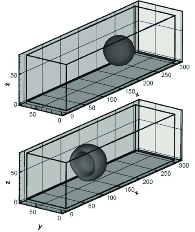
Figure 9: Density iso-surfaces of a high density bubble at $t=0.0$, $0.1$, respectively.

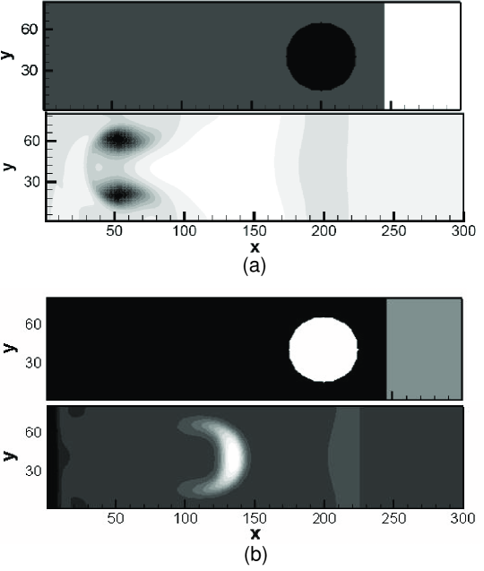
Figure 10: Density contours on section $z=40$ at $t=0.0$, $0.1$. (a) and (b) correspond to the processes of Figure 8 and Figure 9. From black to white, the density value increases.

V Conclusion

We proposed a highly efficient 3D LB model for high-speed compressible flows. The convection term in Boltzmann equation is solved with the finite difference NND method, additional dissipation term is introduced to match the more realistic kinetic viscosity and to be more stable in numerical simulations. Model parameters are controlled in such a way that the von Neumann stability criterion is satisfied. The model can be used to simulate flows from subsonic to supersonic flows, especially supersonic flows with shock waves.

References

- (1) S. Succi, The Lattice Boltzmann Equation for Fluid Dynamics and Beyond, Oxford University Press, New York(2001).
- (2) X. Shan, H. Chen, Phys. Rev. E 47 (1993) 1815; Phys. Rev. E 49 (1994) 2941.
- (3) A.G. Xu, G. Gonnella, and A. Lamura, Phys. Rev. E 74 (2006) 011505; Phys. Rev. E 67 (2003) 056105; Physica A 331 (2004) 10; Physica A 344 (2004) 750; Physica A 362 (2006) 42; A.G. Xu, Commun. Theor. Phys. 39 (2003) 729.
- (4) S.Chen, H.Chen, D.Martinez, and W.Matthaeus, Phys. Rev. Lett., 67 (1991) 3776.
- (5) S.Succi, M.Vergassola and R.Benzi, Phys. Rev. A, 43 (1991) 4521.
- (6) G.Breyiannis and D.Valougeorgis, Phys. Rev. E, 69 (2004) 065702(R).
- (7) A. Gunstensen and D.H. Rothman, J. Geophy. Research 98 (1993) 6431.
- (8) Q. J. Kang, D. X.Zhang, and S. Y.Chen, Phys. Rev. E, 66 (2002) 056307.
- (9) Y. Chen, H. Ohashi, and M. Akiyama, J. Sci. Comp. 12 (1997) 169.
- (10) S.X. Hu, G.W. Yan, W.P. Shi, Acta Mech. Sinica (English Series) 13 (1997) 218.
- (11) G.W. Yan, Y.S. Chen, S.X. Hu, Phys. Rev. E 59 (1999) 454.
- (12) W.P. Shi, W. Shyy, R. Mei, Numer. Heat Transfer, Part B 40 (2001) 1.
- (13) T. Kataoka, M. Tsutahara, Phys. Rev. E 69 (2004) 056702.
- (14) F. Tosi, S. Ubertini, S. Succi, H. Chen, I.V. Karlin, Math. Comput. Simul. 72 (2006) 227.
- (15) V. Sofonea, A. Lamura, G. Gonnella, A. Cristea, Phys. Rev. E 70 (2004) 046702.
- (16) X.F. Pan, A.G. Xu, G.C. Zhang, and S. Jiang, Int. J. Mod. Phys. C 18 (2007) 1747.
- (17) Y.B. Gan, A.G. Xu, G.C. Zhang, X.J. Yu, and Y.J. Li, Physica A 387 (2008) 1721.
- (18) F. Chen, A.G. Xu, G.C. Zhang, Y.B. Gan, T. Cheng, and Y.J. Li, Commun. Theor. Phys., 52 (2009) 681.
- (19) R. A. Brownlee, A. N. Gorban, J. Levesley, Phys. Rev. E 75 (2007) 036711.
- (20) F. Chen, A.G. Xu, G. C. Zhang, Y. J. Li and S. Succi, Europhys. Lett., (in press) [arXiv:1004.5442].
- (21) M. Watari, M. Tsutahara, Physica A 364 (2006) 129.
- (22) Q. Li, Y.L. He, Y. Wang, G.H. Tang, Physics Letters A 373 (2009) 2101.
- (23) P. Bhatnagar, E. P. Gross, and M. K. Krook, Phys. Rev. 94 (1954) 511.
- (24) C. Q. Jin, K. Xu. J. Comput. Phys. 218 (2006) 68.
- (25) D. X. Fu, Y. W. Ma, X. L. Li, Chinese Phys. Lett. 25 (2008) 188.
- (26) J. F. Haas, B. Sturtevant, J. Fluid Nech. 181 (1987) 41.