Towards an SDP-based Approach to Spectral Methods
A Nearly-Linear-Time Algorithm for Graph Partitioning and Decomposition

Abstract

In this paper, we consider the following graph partitioning problem: The input is an undirected graph $G=(V,E),$ a balance parameter $b\in(0,1/2]$ and a target conductance value $\gamma\in(0,1).$ The output is a cut which, if non-empty, is of conductance at most $O(f),$ for some function $f(G,\gamma),$ and which is either balanced or well correlated with all cuts of conductance at most $\gamma.$ In a seminal paper, Spielman and Teng [16] gave an $\tilde{O}(|E|/\gamma^{2})$-time algorithm for $f=\sqrt{\gamma\log^{3}|V|}$ and used it to decompose graphs into a collection of near-expanders [18].

We present a new spectral algorithm for this problem which runs in time $\tilde{O}(|E|/\gamma)$ for $f=\sqrt{\gamma}.$ Our result yields the first nearly-linear time algorithm for the classic Balanced Separator problem that achieves the asymptotically optimal approximation guarantee for spectral methods.

Our method has the advantage of being conceptually simple and relies on a primal-dual semidefinite-programming (SDP) approach. We first consider a natural SDP relaxation for the Balanced Separator problem. While it is easy to obtain from this SDP a certificate of the fact that the graph has no balanced cut of conductance less than $\gamma,$ somewhat surprisingly, we can obtain a certificate for the stronger correlation condition. This is achieved via a novel separation oracle for our SDP and by appealing to Arora and Kale’s [3] framework to bound the running time. Our result contains technical ingredients that may be of independent interest.

1 Introduction

1.1 Graph Partitioning.

Given a graph $G=(V,E),$ the conductance of a cut $(S,\bar{S})$ is $\phi(S)\stackrel{{\scriptstyle\textup{def}}}{{=}}\nicefrac{{|E(S,\bar{S})|}}{{\min\{\mathrm{vol}(S),\mathrm{vol}(\overline{S})\}}},$ where $\mathrm{vol}(S)$ is the sum of the degrees of the vertices in the set $S$. A cut $(S,\bar{S})$ is $b$-balanced if $\min\{\mathrm{vol}(S),\mathrm{vol}(\bar{S})\}\geqslant b\cdot\mathrm{vol}{V}.$ A graph partitioning problem of widespread interest is the Balanced Separator problem: given $G=(V,E),$ a constant balance parameter $b\in(0,\nicefrac{{1}}{{2}}],$ and a conductance value $\gamma\in(0,1),$ does $G$ have a $b$-balanced cut $S$ such that $\phi(S)\leqslant\gamma$?

Balanced Separator is an intensely studied problem in both theory and practice. It has far-reaching connections to spectral graph theory, the study of random walks and metric embeddings. Besides being a theoretically rich problem, Balanced Separator is of great practical importance, as it plays a central role in the design of recursive algorithms, image segmentation and clustering.

Since Balanced Separator is an NP-hard problem [6], we seek approximation algorithms that either output a cut of conductance at-most $f(\gamma,\log|V|)$ and balance $\Omega_{b}(1)$ or a certificate that $G$ has no $b$-balanced cut of conductance at most $\gamma.$ In their seminal series of papers [16, 18, 17], Spielman and Teng use an approximation algorithm for Balanced Separator as a fundamental primitive to decompose the instance graph into a collection of near-expanders. This decomposition is then used to construct spectral sparsifiers and solve systems of linear equations in nearly linear time. Their algorithm has two crucial features: first, it runs in nearly linear time; second, in the case that no balanced cut exists in the graph, it outputs a certificate of a special form. This certificate consists of an unbalanced cut of small conductance which is well-correlated with all low-conductance cuts in the graph. We prove in Section A.1 in the Appendix that such a cut is indeed a negative certificate for the Balanced Separator problem. Formally, they prove the following:

Theorem 1.1

[16] Given a graph $G$, a balance parameter $b\in(0,\nicefrac{{1}}{{2}}],\;b=\Omega(1)$ and a conductance value $\gamma\in(0,1),$ Partition$(G,b,\gamma)$ runs in time $\tau$ and outputs a cut $S\subseteq V$ such that $\mathrm{vol}(S)\leqslant\nicefrac{{7}}{{8}}\cdot\mathrm{vol}(G),$ $\phi(S)\leqslant f_{1}$ or $S=\emptyset,$ and with high probability, either

1. $S$ is $\Omega_{b}(1)$-balanced, or

2. for all $C\subset V$ such that $\mathrm{vol}(C)\leqslant\nicefrac{{1}}{{2}}\cdot\mathrm{vol}(G)$ and $\phi(C)\leqslant O(\gamma),$ $\frac{\mathrm{vol}(S\cap C)}{\mathrm{vol}(C)}\geqslant\nicefrac{{1}}{{2}}.$

Originally, Spielman and Teng showed Theorem 1.1 with $f_{1}=O\left(\sqrt{\gamma\log^{3}n}\right)$ and $\tau=\tilde{O}\left(\nicefrac{{m}}{{\gamma^{2}}}\right).$ This was subsequently improved by Andersen, Chung and Lang [1] and then by Andersen and Peres [2] to the current best of $f_{1}=O\left(\sqrt{\gamma\log n}\right)$ and $\tau=\tilde{O}(\nicefrac{{m}}{{\sqrt{\gamma}}}).$ All these results made use of bounds on the convergence of random walk processes on the instance graph, such as the Lovasz-Simonovits bounds [13]. These bounds yield the $\log n$ factor in the approximation guarantee, which appears hard to remove while following this approach.

1.2 Our Contribution

In this paper, we use a semidefinite programming approach to design a new spectral algorithm, called BalCut, that improves on the result of Theorem 1.1. The following is our main result.

Theorem 1.2 (Main Theorem)

Given a graph $G=(V,E)$, a balance parameter $b\in(0,\nicefrac{{1}}{{2}}],\;b=\Omega(1),$ and a conductance value $\gamma\in(0,1),$ BalCut$(G,b,\gamma)$ runs in time $\tilde{O}\left(\nicefrac{{m}}{{\gamma}}\right)$ and outputs a cut $S\subset V$ such that $\mathrm{vol}(S)\leqslant\nicefrac{{7}}{{8}}\cdot\mathrm{vol}(G),$ if $S\neq\emptyset$ then $\phi(S)\leqslant O_{b}\left(\sqrt{\gamma}\right),$ and with high probability, either

1. $S$ is $\Omega_{b}(1)$-balanced, or

2. for all $C\subset V$ such that $\mathrm{vol}(C)\leqslant\nicefrac{{1}}{{2}}\cdot\mathrm{vol}(G)$ and $\phi(C)\leqslant O(\gamma),$ $\frac{\mathrm{vol}(S\cap C)}{\mathrm{vol}(C)}\geqslant\nicefrac{{1}}{{2}}.$

Note that our result improves the parameters of previous algorithms by eliminating the $\log n$ factor in the quality of the cut output, making the approximation comparable to the best that can be hoped for using spectral methods [7]. Our result is also conceptually simple: we use the primal-dual framework of Arora and Kale [3] to solve SDPs combinatorially, and we give a new separation oracle that yields Theorem 1.2. Finally, our result implies an approximation algorithm for Balanced Separator, as the guarantee of Theorem 1.2 on the cut $S$ output by BalCut also implies a lower bound on the conductance of balanced cuts of $G.$ The proof can be found in Section A.1 in the Appendix.

Corollary 1.1

Given an instance graph $G,$ a balance parameter $b\in(0,\nicefrac{{1}}{{2}}]$ and a target conductance $\gamma\in(0,1],$ BalCut $(G,b,\gamma)$ either outputs an $\Omega_{b}(1)$-balanced cut of conductance at most $O_{b}(\sqrt{\gamma})$ or a certificate that all $\Omega_{b}(1)$-balanced cuts have conductance at least $\Omega_{b}(\gamma).$ The running time of the algorithm is $\tilde{O}(m/{\gamma}).$

This is the first nearly-linear-time spectral algorithm for Balanced Separator that achieves the asymptotically optimal approximation guarantee for spectral methods.

1.3 Graph Decomposition.

The main application of Theorem 1.1 is the construction of a particular kind of graph decomposition. In this decomposition, we wish to partition the vertex set of the instance graph $V$ into components $V_{1},\ldots,V_{i},\ldots,V_{k}$ such that the graph induced by $G$ on each $V_{i}$ has conductance as large as possible, while at most a constant fraction of the edges have endpoints in different components. These decompositions are a useful algorithmic tool in several areas [20, 11, 18].

Kannan, Vempala and Vetta [10] construct such decompositions achieving a conductance value of $\Omega(\nicefrac{{1}}{{\log^{2}n}}).$ However, their algorithm runs in time $\tilde{O}(m^{2})$ on some instances.

Spielman and Teng [18] relax this notion of decomposition by only requiring that each $V_{i}$ be contained in a superset $W_{i}$ in $G$, where $W_{i}$ has large induced conductance in $G.$ In the same work, they show that this relaxed notion of decomposition suffices for the purposes of sparsification by random sampling. The advantage of this relaxation is that it is now possible to compute this decomposition in nearly-linear time by recursively applying the algorithm of Theorem 1.1.

Theorem 1.3

[18] Assume the existence of an algorithm achieving parameters $\tau$ and $f_{1}$ in Theorem 1.1. Given $\gamma\in(0,1),$ in time $\tilde{O}(\tau),$ it is possible to construct a decompositions of the instance graph $G$ into components $V_{1},\ldots,V_{k}$ such that:

1. for each $V_{i},$ there exists $W_{i}\supseteq V_{i}$ such that the conductance of the graph induced by $G$ on $W_{i}$ is $\Omega(\nicefrac{{\gamma}}{{\log n}}).$

2. the fraction of edges with endpoints in different components is $O(f_{1}\log n).$

Using Theorem 1.3, Spielman and Teng showed the existence of a decomposition achieving conductance $\Omega(\nicefrac{{1}}{{\log^{6}n}}).$ Our improved results in Theorem 1.2 imply that we can obtain decompositions of the same kind with conductance bound $\Omega(\nicefrac{{1}}{{\log^{3}n}}).$ Our improvement also implies speed-ups in the sparsification procedure described by Spielman and Teng [18]. However, this result has since been superceded by work of Koutis, Miller and Peng [12] that gives a very fast linear equation solver that can be used to compute sampling probabilities for each edge, yielding a spectral sparsifier with high probability [15].

Our work leaves open the important question posed by Spielman [14] of whether stronger decompositions, of the kind proposed by Kannan, Vempala and Vetta [10], can be produced in nearly-linear time.

1.4 Overview of Techniques

Spectral Approach.

The simplest algorithm for Balanced Separator, also used by Kannan et al. [10], is the recursive spectral algorithm. This algorithm finds the minimum-conductance sweep cut of the second eigenvector of $G$, removes the cut and all adjacent edges from $G,$ and reiterates on the remaining graph. The algorithm stops when the union of the cuts removed becomes $\nicefrac{{b}}{{2}}$-balanced or when the residual graph is found to have spectral gap at least $\gamma,$ certifying that no more progress can be made. As every cut may only remove $O(1)$ volume and the eigenvector computation takes $\Omega(m)$ time, this algorithm may have quadratic running time. It can be shown using Cheeger’s Inequality [5] that the cut this procedure outputs is of conductance at most $O(\sqrt{\gamma}).$

Spielman-Teng Approach.

The algorithm of Spielman and Teng which proves Theorem 1.1 is also spectral in nature and uses, as the main subroutine, local random walks that run in time proportional to the volume of the output cut to find sparse cuts around vertices of the graphs. These local methods are based on non-trivial random walks on the input graph and aggregation of the information obtained from these walks, all performed while maintaining nearly-linear running time.

Our Approach.

We depart from the random-walk paradigm and first consider a natural SDP relaxation for the Balanced Separator problem, which BalCut solves approximately using a primal-dual method. Intuitively, BalCut manages to maintain the approximation guarantee of the recursive spectral algorithm while running in nearly-linear time by considering a distribution over eigenvectors, represented as a vector embedding of the vertices, rather than a single eigenvector, at each iteration. The sweep cut over the eigenvector is replaced by a sweep cut over the radius of the vectors in the embedding (see Figure 1). Moreover, at any iteration, rather than removing the unbalanced cut found, BalCut penalizes it by modifying the graph so that it is unlikely but still possible for it to turn up in future iterations. Hence, in both its cut-finding and cut-eliminating procedures, BalCut tends to “hedge its bets” more than the greedy recursive spectral method. This hedging, which ultimately allows BalCut to achieve its faster running time, is implicit in the primal-dual framework of Arora and Kale [3].

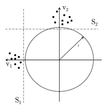
Figure 1: Schematic representation of the speed-up introduced by BalCut when the instance graph contains many unbalanced cuts of low conductance. Let $v_{1}$ and $v_{2}$ be the two slowest-mixing eigenvectors of $G.$ Assume that their minimum-conductance sweep cuts $S_{1}$ and $S_{2}$ are unbalanced cuts of conductance less than $\gamma.$ If we use the recursive algorithm of Kannan et al. [10], two iterations could be required to remove $S_{1}$ and $S_{2}$. However, BalCut considers a multidimensional embedding containing contributions from multiple eigenvectors and performs a radial sweep cut. This allows $S_{1}$ and $S_{2}$ to be removed in a single iteration.

The SDP relaxation appears in Figure 2. We denote by $\mu:V\mapsto\varmathbb{R}_{\geqslant 0}$ the distribution defined as $\mu_{i}\stackrel{{\scriptstyle\textup{def}}}{{=}}\nicefrac{{d_{i}}}{{\mathrm{vol}(G)}},$ and by $d_{i}$ the degree of the $i$-th vertex. Also, $v_{avg}\stackrel{{\scriptstyle\textup{def}}}{{=}}\sum_{i}\mu_{i}v_{i}.$ Even though our algorithm uses the SDP, at the core, it is spectral in nature, as it relies on the matrix-vector multiplication primitive. Hence, if one delves deeper, a random walk interpretation can be derived for our algorithm.

$${{\mathsf{psdp}}}(G,b,\gamma): \cdot\operatorname*{\varmathbb{E}}_{\{i,j\}\in E}\;\lVert v_{i}-v_{j}\rVert_{2}^{2}\;\leqslant \;\gamma$$ /14

$$\operatorname*{\varmathbb{E}}_{j\sim\mu}\;\lVert v_{j}-v_{\mathsf{avg}}\rVert_{2}^{2}\;= \;1$$

$$\forall{i\in V}\; \lVert v_{i}-v_{\mathsf{avg}}\rVert_{2}^{2}\;\leqslant \;\frac{(1-b)}{b}$$

Figure 2: SDP for $b$-Balanced Separator

The Primal-Dual Framework.

For our SDP, the method of Arora and Kale can be understood as a game between two players: an embedding player and an oracle player. The embedding player, in every round of this game, gives a candidate vector embedding of the vertices of the instance graph to the oracle player. We show that, if we are lucky and the embedding is feasible for the SDP and, in addition, also has the property that for a large set $S,$ for every $i\in S,$ $\|v_{i}-v_{avg}\|_{2}\leqslant O(\nicefrac{{(1-b)}}{{b}})$ (we call such an embedding roundable), then a projection of the vectors along a random direction followed by a sweep cut gives an $\Omega_{b}(1)$-balanced cut of conductance at most $O(\sqrt{\gamma}).$ The difficult case is when the embedding given to the oracle player is not roundable. In this case, the oracle outputs a candidate dual solution along with a cut. The oracle obtains this cut by performing a radial sweep cut of the vectors given by the embedding player. If at any point in this game the union of cuts output by the oracle becomes balanced, we output this union and stop. We show that such a cut is of conductance at most $O_{b}(\sqrt{\gamma}).$ If this union of cuts is not balanced, then the embedding player uses the dual solution output by the oracle to update the embedding. Finally, the matrix-exponential update rule ensures that this game cannot keep on going for more that $O(\nicefrac{{\log n}}{{/}}{\gamma})$ rounds. Hence, if a balanced cut is not found after this many rounds, we certify that the graph does not contain any $b$-balanced cut of conductance less than $\gamma.$ To achieve a nearly-linear running time, we maintain only a $\log n$-dimensional sketch of the embedding. The guarantee on the running time then follows by noticing that, in each iteration, the most expensive computational step for each player is a logarithmic number of matrix-vector multiplications, which takes at most $\tilde{O}(m)$ time.

The reason why our approach yields the desired correlation condition in Theorem 1.2 is that, if no balanced cut is found, every unbalanced cut of conductance lower than $\gamma$ will, at some iteration, have a lot of its vertices mapped to vectors of large radius. At that iteration, the cut output by the oracle player will have a large correlation with the target cut, which implies that the union of cuts output by the oracle player will also display such large correlation. This intuition is formalized in the proof of Theorem 1.2.

Our Contribution.

The implementation of the oracle player, specifically dealing with the case when the embedding is not roundable, is the main technical novelty of the paper. Studying the problem in the SDP-framework is the main conceptual novelty. The main advantage of using SDPs to design a spectral algorithm seems to be that SDP solutions provide a simple representation for possibly complex random-walk objects. Furthermore, the benefits of using a carefully designed SDP formulation can often be reaped with little or no burden on the running time of the algorithm, thanks to the primal-dual framework of Arora and Kale [3].

1.5 Rest of the Paper

In Section 2.1, we set the notation for the paper. In Section 2.2, we present our SDP and its dual, and also define the notion of a roundable embedding. In Section 2.3, we present the algorithm BalCut and the separation oracle Oracle, and reduce the task of proving Theorem 1.2 to proving statements about the Oracle. Section 3 contains the proof of the main theorem about the Oracle used in Section 2.3. For clarity of presentation, several proofs are omitted from the above sections and appear in the appendix.

2 Algorithm Statement and Main Theorems

2.1 Notation

Instance graph and edge volume.

We denote by $G=(V,E)$ the unweighted instance graph, where $\lvert V\rvert=n$ and $\lvert E\rvert=m.$ We let $d\in\varmathbb R^{V},$ be the degree vector of $G,$ i.e. $d_{i}$ is the degree of vertex $i.$ We mostly work with the edge measure $\mu$ over $V,$ defined as $\mu_{i}\stackrel{{\scriptstyle\textup{def}}}{{=}}\mu(i)\stackrel{{\scriptstyle\textup{def}}}{{=}}\nicefrac{{d_{i}}}{{2m}}.$ For a subset $S\subseteq V,$ we also define $\mu_{S}$ as the edge measure over $S$, i.e. $\mu_{S}(i)\stackrel{{\scriptstyle\textup{def}}}{{=}}\nicefrac{{\mu(i)}}{{\mu(S)}}.$

Special graphs

For a subset $S\subseteq V,$ we denote by $K_{S}$ the complete graph over $S$ such that edge $\{i,j\}$ has weight $\mu_{i}\mu_{j}$ for $i,j\in S$ and $0$ otherwise. $K_{V}$ is the complete graph with weight $\mu_{i}\mu_{j}$ between every pair $i,j\in V.$

Graph matrices.

For an undirected graph $H=(V,E_{H})$, let $A(H)$ denote the adjacency matrix of $H$ and $D(H)$ the diagonal matrix of degrees of $H$. The (combinatorial) Laplacian of $H$ is defined as $L(H)\stackrel{{\scriptstyle\textup{def}}}{{=}}D(H)-A(H)$. Note that for all $x\in\varmathbb R^{V}$, $x^{T}L(H)x=\sum_{\{i,j\}\in E_{H}}(x_{i}-x_{j})^{2}$. By $D$ and $L$, we denote $D(G)$ and $L(G)$ respectively.

Vector and matrix notation.

For a symmetric matrix $M,$ we will use $M\succeq 0$ to denote that it is positive semi-definite and $M\succ 0$ to denote that it is positive definite. The expression $A\succeq B$ is equivalent to $A-B\succeq 0$. For two matrices $A,B$ of equal dimensions, denote $A\bullet B\stackrel{{\scriptstyle\textup{def}}}{{=}}{\rm Tr}(A^{T}B)=\sum_{ij}A_{ij}\cdot B_{ij}.$ For a matrix $A$, we indicate by $t_{A}$ the time necessary to compute the matrix-vector multiplications $Au$ for any vector $u$.

Embedding notation.

We will deal with vector embeddings of $G$, where each vertex $i\in V$ is mapped to a vector $v_{i}\in\varmathbb R^{d}.$ For such an embedding $\{v_{i}\}_{i\in V},$ we denote by $v_{\mathsf{avg}}$ the mean vector, i.e. $v_{\mathsf{avg}}\stackrel{{\scriptstyle\textup{def}}}{{=}}\sum_{i\in V}\mu_{i}v_{i}.$ Given a vector embedding of $\{v_{i}\in\varmathbb R^{d}\}_{i\in V},$ recall that $X\succeq 0,$ is the Gram matrix of the embedding if $X_{ij}=v_{i}^{T}v_{j}.$ For any $X\in\varmathbb R^{V\times V},X\succeq 0,$ we call $\{v_{i}\}_{i\in V}$ the embedding corresponding to $X$ if $X$ is the Gram matrix of $\{v_{i}\}_{i\in V}.$ For $i\in V,$ we denote by $R_{i}$ the matrix such that $R_{i}\bullet X=\lVert v_{i}-v_{\mathsf{avg}}\rVert_{2}^{2}.$

Basic facts.

We will alternatively use vector and matrix notation to reason about the graph embeddings. The following are some simple conversions between vectors and matrix forms and some basic geometric facts which follow immediately from definitions.

Fact 2.1

$\operatorname*{\varmathbb{E}}_{i\sim\mu}\lVert v_{i}-v_{\mathsf{avg}}\rVert_{2}^{2}=\nicefrac{{1}}{{2}}\cdot\operatorname*{\varmathbb{E}}_{\{i,j\}\sim\mu\times\mu}\lVert v_{i}-v_{j}\rVert_{2}^{2}=L(K_{V})\bullet X.$

Fact 2.2

For a subset $S\subseteq V,$ $\sum_{i\in S}\mu_{i}R_{i}\succeq\mu(S)L(K_{V})-L(K_{S}).$

Fact 2.3

For a subset $S\subseteq V,$ $\operatorname*{\varmathbb{E}}_{\{i,j\}\sim\mu_{S}\times\mu_{S}}\lVert v_{i}-v_{j}\rVert_{2}^{2}=2\cdot\nicefrac{{1}}{{\mu(S)^{2}}}\cdot L(K_{S})\bullet X.$

Modified matrix exponential update.

Let $\mathcal{S}_{D}$ e the subspace of $\varmathbb R^{V}$ orthogonal to $\hat{v}\stackrel{{\scriptstyle\textup{def}}}{{=}}\nicefrac{{1}}{{\sqrt{2m}}}\cdot D^{\nicefrac{{1}}{{2}}}1$ and let $\mathcal{I}$ be the identity over $\mathcal{S}_{D},$ i.e. $\mathcal{I}\stackrel{{\scriptstyle\textup{def}}}{{=}}I-\nicefrac{{1}}{{2m}}\cdot D^{\nicefrac{{1}}{{2}}}11^{T}D^{\nicefrac{{1}}{{2}}}.$ For a positive $\varepsilon$ and a symmetric matrix $M\in\varmathbb R^{V\times V},$ we define

$$U_{\varepsilon}(A)\stackrel{{\scriptstyle\textup{def}}}{{=}}2m\cdot\frac{D^{-\nicefrac{{1}}{{2}}}e^{-(2m\cdot\varepsilon)\cdot D^{-\nicefrac{{1}}{{2}}}MD^{-\nicefrac{{1}}{{2}}}}D^{-\nicefrac{{1}}{{2}}}}{\mathcal{I}\bullet e^{-(2m\cdot\varepsilon)D^{-\nicefrac{{1}}{{2}}}MD^{-\nicefrac{{1}}{{2}}}}}.$$

The following fact about $\mathcal{I}$ will also be needed:

Fact 2.4

$\mathcal{I}=2m\cdot D^{-\nicefrac{{1}}{{2}}}L(K_{V})D^{-\nicefrac{{1}}{{2}}}.$

2.2 SDP Formulation

We consider an ${\sf SDP}$ relaxation to the decision problem of determining whether the instance graph $G$ has a $b$-balanced cut of conductance at most $\gamma.$ The ${\sf SDP}$ feasibility program ${{\mathsf{psdp}}}(G,b,\gamma)$ appears in Figure $\ref{fig:sdp},$ where we also rewrite the program in matrix notation, using Fact 2.1 and the definition of $R_{i}.$

$${{\mathsf{psdp}}}(G,b,\gamma): \operatorname*{\varmathbb{E}}_{\{i,j\}\in E}\;\lVert v_{i}-v_{j}\rVert_{2}^{2}\;\leqslant \;4\gamma$$

$$\operatorname*{\varmathbb{E}}_{j\sim\mu}\;\lVert v_{j}-v_{\mathsf{avg}}\rVert_{2}^{2}\;= \;1$$

$$\forall i\in V\; \lVert v_{i}-v_{\mathsf{avg}}\rVert_{2}^{2}\;\leqslant \;\frac{1-b}{b}$$

$${{\mathsf{psdp}}}(G,b,\gamma): \frac{1}{m}\cdot L\bullet X\;\leqslant \;4\gamma$$

$$L(K_{V})\bullet X\;= \;1$$

$$\forall i\in V R_{i}\bullet X\;\leqslant \;\frac{1-b}{b}$$

Figure 3: ${\sf SDP}$ for $b$-Balanced Separator

${{\mathsf{psdp}}}$ can be seen as a scaled version of the balanced-cut ${\sf SDP}$ of [4], modified by replacing $v_{\mathsf{avg}}$ for the origin and removing the triangle-inequality constraints. The first change makes our ${{\mathsf{psdp}}}$ invariant under translation of the embeddings and makes the connection to spectral methods more explicit. Indeed, the first two constraints of ${\mathsf{psdp}}$now exactly correspond to the standard eigenvector problem, with the addition of the $R_{i}$ constraint ideally forcing all entries in the eigenvector not to be too far from the mean, just as it would be the case if the eigenvector exactly corresponded to a balanced cut. The removal of the triangle-inequality constraints causes ${{\mathsf{psdp}}}$ to only deal with the spectral structure of $L$ and not to have a flow component. For the rest of the paper, denote by $\Delta$ the set $\{X\in\varmathbb R^{V\times V},X\succeq 0:L(K_{V})\bullet X=1\}.$

The following simple lemma establishes that ${{\mathsf{psdp}}}$ is indeed a relaxation for the integral decision question and is proved in Section A.2.

Lemma 2.1 (SDP is a Relaxation)

If there exists a $b$-balanced cut $S$ with $\phi(S)\leqslant\gamma,$ then ${{\mathsf{psdp}}}(G,b,\gamma)$ has a feasible solution.

BalCut will use the primal-dual approach of [3] to determine the feasibility of ${{\mathsf{psdp}}}(G,b,\gamma).$ When ${\mathsf{psdp}}$is infeasible, BalCut will output a solution to the dual ${\mathsf{dsdp}}(G,b,\gamma),$ shown in Figure 4.

$${\mathsf{dsdp}}(G,b,\gamma):\quad \alpha-\frac{1-b}{b}\sum_{i\in V}\beta_{i}>4\gamma$$

$$\frac{1}{2m}\cdot L+\sum_{i\in V}\beta_{i}R_{i}-\alpha L(K_{V})\succeq 0$$

$$\alpha\in\varmathbb R,\;\;\beta\geqslant 0$$

Figure 4: ${\mathsf{dsdp}}(G,b,\gamma)$ feasibility problem

In the rest of the paper, we are going to use the following shorthands for the dual constraints

$$V(\alpha,\beta)\stackrel{{\scriptstyle\textup{def}}}{{=}}\alpha-\frac{1-b}{b}\sum_{i\in V}\beta_{i},\;M(\alpha,\beta)\stackrel{{\scriptstyle\textup{def}}}{{=}}\frac{L}{2m}+\sum_{i\in V}\beta_{i}R_{i}-\alpha L(K_{V}).$$

Notice that $V(\alpha,\beta)$ is a scalar, while $M(\alpha,\beta)$ is a matrix in $\varmathbb{R}^{V\times V}.$ Given $X\succeq 0,$ a choice of $(\alpha,\beta)$ such that $V(\alpha,\beta)>4\gamma$ and $M(\alpha,\beta)\bullet X\geqslant 0$ corresponds to a hyperplane separating $X$ from the feasible region of ${{\mathsf{psdp}}}(G,b,\gamma)$ and constitutes a certificate that $X$ is not feasible.

Ideally, BalCut would produce a feasible solution to ${\mathsf{psdp}}$and then round it to a balanced cut. However, as discussed in [3], it often suffices to find a solution “close” to feasible for the rounding procedure to apply. In the case of ${\mathsf{psdp}}$, the concept of “closeness” is captured by the notion of roundable solution.

Definition 2.1 (Roundable Embedding)

Given an embedding $\{v_{i}\}_{i\in V},$ let $R=\{i\in V:\lVert v_{i}-v_{\mathsf{avg}}\rVert_{2}^{2}\leqslant 32\cdot\nicefrac{{(1-b)}}{{b}}\}.$ We say that $\{v_{i}\}_{i\in V}$ is a roundable solution to ${{\mathsf{psdp}}}(G,b,\gamma)$ if:

• $\operatorname*{\varmathbb{E}}_{\{i,j\}\in E}\;\lVert v_{i}-v_{j}\rVert_{2}^{2}\;\leqslant\;2\gamma$,

• $\operatorname*{\varmathbb{E}}_{j\sim\mu}\;\lVert v_{j}-v_{\mathsf{avg}}\rVert_{2}^{2}\;=\;1$,

• $\operatorname*{\varmathbb{E}}_{\{i,j\}\sim\mu_{R}\times\mu_{R}}\lVert v_{i}-v_{j}\rVert_{2}^{2}\geqslant\nicefrac{{1}}{{64}}.$

A roundable embedding can be converted into a balanced cut of the conductance required by Theorem 1.2 by using a standard projection rounding, which is a simple extension of an argument already appearing in [4] and [3]. The rounding procedure ProjRound is described precisely in Section A.4, where the following theorem is proved.

Theorem 2.1 (Rounding Roundable Embeddings)

If $\{v_{i}\in\varmathbb R^{d}\}_{i\in V}$ is a roundable solution to ${{\mathsf{psdp}}}(G,b,\gamma)$, then ProjRound$(\{v_{i}\}_{i\in V},b)$ produces a $\Omega_{b}(1)$- balanced cut of conductance $O_{b}\left(\sqrt{\gamma}\right)$ with high probability in time $\tilde{O}(nd+m).$

2.3 Primal-Dual Framework

Input: An instance graph $G=(V,E),$ a balance value $b\in(0,\nicefrac{{1}}{{2}}]$ such that $b=\Omega(1),$ a conductance value $\gamma\in(0,1).$ Let $\varepsilon=\nicefrac{{1}}{{130}}.$ For $t=1,2,\ldots,T=O\left(\frac{\log n}{\gamma}\right):$ – Compute the embedding $\{\tilde{v}^{(t)}_{i}\}_{i\in V}$ corresponding to $\tilde{X}^{(t)}=\tilde{U}_{\varepsilon}\left(\sum_{j=1}^{t-1}P^{(j)}\right).$ If $t=1,$ $\tilde{X}^{(1)}=\tilde{U}_{\varepsilon}\left(0\right)=\nicefrac{{2m}}{{n-1}}\cdot D^{-1}.$ – Execute Oracle$\left(G,b,\gamma,\{\tilde{v}^{(t)}_{i}\}_{i\in V}\right).$ – If Oracle finds that $\{\tilde{v}^{(t)}_{i}\}_{i\in V}$ is roundable, run ProjRound$\left(G,b,\{\tilde{v}^{(t)}_{i}\}_{i\in V}\right),$ output the resulting cut and terminate. – Otherwise, Oracle outputs coefficients $\left(\alpha^{(t)},\beta^{(t)}\right)$ and cut $B^{(t)}.$ – Let $C^{(t)}\stackrel{{\scriptstyle\textup{def}}}{{=}}\bigcup_{i=1}^{t}B^{(i)}.$ If $C^{(t)}$ is $\nicefrac{{b}}{{4}}$-balanced, output $C^{(t)}$ and terminate. – Otherwise, let $P^{(t)}\stackrel{{\scriptstyle\textup{def}}}{{=}}-\nicefrac{{\varepsilon}}{{6}}\cdot\left(M\left(\alpha^{(t)},\beta^{(t)}\right)+\gamma L(K_{V})\right)$ and proceed to the next iteration. Output $S=\bigcup_{t=1}^{T}B^{(t)}.$ Also output $\bar{\alpha}=\nicefrac{{1}}{{T}}\sum_{t=1}^{T}\alpha^{(t)}$ and $\bar{\beta}=\nicefrac{{1}}{{T}}\sum_{t=1}^{T}\beta^{(t)}.$

Figure 5: The BalCut Algorithm

Separation Oracle.

The problem of checking the feasibility of a SDP can be reduced to that of, given a candidate solution $X,$ to check whether it is close to feasible and, if not, provide a certificate of infeasibility in the form of a hyperplane separating $X$ from the feasible set. The algorithm performing this computation is known as a separation oracle. Arora and Kale show that the original feasiblity problem can be solved very efficiently if there exists a separation oracle obeying a number of conditions. We introduce the concept of good separation oracle to capture these conditions for the program ${{\mathsf{psdp}}}(G,\beta,\gamma).$

Definition 2.2 (Good Separation Oracle)

An algorithm is a good separation oracle if, on input some representation of $X,$ the algorithm either finds $X$ to be a roundable solution to ${{\mathsf{psdp}}}(G,b,\gamma)$ or outputs coefficents $\alpha,\beta$ such that $V(\alpha,\beta)\geqslant\nicefrac{{3}}{{4}}\cdot\gamma,$ $M(\alpha,\beta)\bullet X\geqslant\nicefrac{{1}}{{64}}\cdot\gamma$ and $-\gamma L(K_{V})\preceq M(\alpha,\beta)\preceq 3L(K_{V}).$

Algorithmic Scheme.

We adapt the techniques of [3] to our setting, where we require feasible solutions to be in $\Delta$ rather than having trace equal to 1. The argument is a simple modification of the anaylsis of [3] and in [19]. The algorithmic strategy of [3] is to produce a sequence of candidate primal solutions $X^{(1)},\ldots,X^{(T)}$ iteratively, such that $X^{(t)}\in\Delta$ for all $t.$

Our starting point $X^{(1)}$ will be the solution $\nicefrac{{2m}}{{n-1}}\cdot D^{-1}.$ At every iteration, a good separation oracle Oracle will take $X^{(t)}$ and either guarantee that $X^{(t)}$ is roundable or output coefficents $\alpha^{(t)},\beta^{(t)}$ certifying the infeasiblity of $X^{(t)}.$ The algorithm makes use of the information contained in $\alpha^{(t)},\beta^{(t)}$ by updating the next candidate solution as follows:

(2.1) $$P^{(t)}\stackrel{{\scriptstyle\textup{def}}}{{=}}-\nicefrac{{\varepsilon}}{{6}}\cdot\left(M(\alpha^{(t)},\beta^{(t)})+\gamma L(K_{V})\right)$$

$$X^{(t+1)}\stackrel{{\scriptstyle\textup{def}}}{{=}}U_{\varepsilon}\left(\sum_{i=1}^{t}P^{(i)}\right)$$

where $\varepsilon>0$ is a parameter of the algorithm. The following is immediate.

Lemma 2.2

For all $t>0,$ $X^{(t)}\in\Delta.$

Following [3], we prove that, after a small number of iterations this algorithm either yields a roundable embedding or a feasible solution to $\mathsf{dsdp}$$(G,b,\Omega(\gamma)).$ We present the proof in Section A.3 for completeness.

Theorem 2.2 (Iterations of Oracle, [3])

Let $\varepsilon=\nicefrac{{1}}{{130}}.$ Assume that the procedure Oracle is a good separation oracle . Then, after $T=O\left(\nicefrac{{\log n}}{{\gamma}}\right)$ iterations of the update of Equation 2.1, we either find a roundable solution to ${{\mathsf{psdp}}}(G,b,\gamma)$ or the coefficents $\bar{\alpha}=\nicefrac{{1}}{{T}}\sum_{t=1}^{T}\alpha^{(t)}$ and $\bar{\beta}=\nicefrac{{1}}{{T}}\sum_{t=1}^{T}\beta^{(t)}$ are a feasible solution to ${\mathsf{dsdp}}(G,b,\nicefrac{{3}}{{16}}\cdot\gamma).$

Approximate Computation.

Notice that, while we are seeking to construct a nearly-linear-time algorithm, we cannot hope to compute $X^{(t)}$ exactly and explicitly, as just maintaining the full $X^{(t)}$ matrix requires quadratic time in $n.$ Instead, we settle for a approximation $\tilde{X}^{(t+1)}$ to $X^{(t+1)}$ which we define as

$$\tilde{X}^{(t+1)}=\tilde{U}_{\varepsilon}\left(\sum_{i=1}^{t}P^{(i)}\right).$$

The function $\tilde{U}_{\varepsilon}$ is a randomized approximation to $U_{\varepsilon}$ obtained by applying the Johnson-Linderstrauss dimension reduction to the embedding corresponding to $U_{\varepsilon}.$ $\tilde{U}_{\varepsilon}$ is described in full in Section A.5, where we also prove the following lemma about the accuracy and sparsity of the approximation. It is essentially the same argument appearing in [9] applied to our context.

Lemma 2.3 (Approximate Computation)

Let $\varepsilon=\nicefrac{{1}}{{130}}.$ For a matrix $M\in\varmathbb R^{V\times V},$ $M\succeq 0,$ let $\tilde{X}\stackrel{{\scriptstyle\textup{def}}}{{=}}\tilde{U}_{\varepsilon}(M)$ and $X\stackrel{{\scriptstyle\textup{def}}}{{=}}U_{\varepsilon}(M).$

1. $\tilde{X}\succeq 0$ and $\tilde{X}\in\Delta.$

2. The embedding $\{\tilde{v}_{i}\}_{i\in V}$ corresponding to $\tilde{X}$ can be represented in $d=O(\log n)$ dimensions.

3. $\{\tilde{v}_{i}\in\varmathbb R^{d}\}_{i\in V}$ can be computed in time $\tilde{O}(t_{M}+n).$

4. for any graph $H=(V,E_{H})$, with high probability

   $$(1-\nicefrac{{1}}{{64}})\cdot L(H)\bullet X-\tau\leqslant L(H)\bullet\tilde{X}\leqslant(1+\nicefrac{{1}}{{64}})\cdot L(H)\bullet X+\tau,$$

   and, for any vertex $i\in V,$

   $$(1-\nicefrac{{1}}{{64}})\cdot R_{i}\bullet X-\tau\leqslant R_{i}\bullet\tilde{X}\leqslant(1+\nicefrac{{1}}{{64}})\cdot R_{i}\bullet X+\tau,$$

where $\tau\leqslant O(\nicefrac{{1}}{{\mathrm{poly}(n)}}).$

This lemma shows that $\tilde{X}^{(t)}$ is a close approximation to $X^{(t)}.$ We will use this lemma to show that Oracle can receive $\tilde{X}^{(t)}$ as input, rather than $X^{(t)},$ and still meet the conditions of Theorem 2.2. In the rest of the paper, we assume that $\tilde{X}^{(t)}$ is represented by its corresponding embedding $\{\tilde{v}^{(t)}_{i}\}_{i\in V}.$

The Oracle.

Oracle is described in Figure 6. We show that Oracle on input $\tilde{X}^{(t)}$ meets the condition of Theorem 2.2. Moreover, we show that Oracle obeys an additional condition, which, combined with the dual guarantee of Theorem 2.2 will yield the correlation property of BalCut.

Theorem 2.3 (Main Theorem on Oracle)

On input $\tilde{X}^{(t)},$ Oracle runs in time $\tilde{O}(m)$ and is a good separation oracle for $X^{(t)}.$ Moreover, the cut $B$ in Step 4 is guaranteed to exist.

1. Input: The embedding $\{\tilde{v}_{i}\}_{i\in V},$ corresponding to $\tilde{X}\in\Delta.$ Let $r_{i}=\lVert\tilde{v}_{i}-\tilde{v}_{\mathsf{avg}}\rVert_{2}$ for all $i\in V.$ Denote $R\stackrel{{\scriptstyle\textup{def}}}{{=}}\{i\in V:r_{i}^{2}\leqslant 32\cdot\nicefrac{{(1-b)}}{{b}}\}.$ 2. Case 1: $\operatorname*{\varmathbb{E}}_{\{i,j\}\in E}\;\lVert\tilde{v}_{i}-\tilde{v}_{j}\rVert_{2}^{2}\geqslant 2\gamma.$ Output $\alpha=\gamma,$ $\beta=0$ and $B=\emptyset.$ 3. Case 2: not Case 1 and $\operatorname*{\varmathbb{E}}_{\{i,j\}\sim\mu_{R}\times\mu_{R}}\lVert v_{i}-v_{j}\rVert_{2}^{2}\geqslant\delta.$ Then $\{\tilde{v}_{i}\}_{i\in V}$ is roundable, as $\tilde{X}\in\Delta$ implies $\operatorname*{\varmathbb{E}}_{j\sim\mu}\;r_{j}^{2}=1.$ 4. Case 3: not Case 1 or 2. Relabel the vertices of $V$ such that $r_{1}\geqslant r_{2}\geqslant\ldots\geqslant r_{n}$ and let $S_{i}=\{1,\ldots,i\}$ be the $j$-th sweep cut of $r.$ Let $z$ the smallest index such that $\mu(S_{z})\geqslant\nicefrac{{b}}{{8}}.$ Let $B$ the most balanced sweep cut among $\{S_{1},\ldots,S_{z-1}\}$ such that $\phi(B)\leqslant 2048\cdot\sqrt{\gamma}.$ Output $\alpha=\nicefrac{{7}}{{8}}\gamma,$ $\beta_{i}=\mu_{i}\cdot\gamma$ for $i\in B$ and $\beta_{i}=0$ for $i\notin B.$ Also output the cut $B.$

Figure 6: Oracle

Proof of Main Theorem.

We are now ready to prove Theorem 1.2. To show the overlap condition, we consider the dual condition implied by Theorem 2.2 together with the cut $B^{(t)}$ and the values of the coefficents output by the Oracle.

• [Proof of Theorem 1.2] If at any iteration $t,$ the embedding $\{\tilde{v}_{i}^{(t)}\}_{i\in V}$ corresponding to $\tilde{X}^{(t)}$ is roundable, the standard projection rounding ProjRound produces a cut of balance $\Omega_{b}(1)$ and conductance $O_{b}(\sqrt{\gamma})$ by Theorem 2.1. Similarly, if for any $t,$ $C^{(t)}$ is $\nicefrac{{b}}{{4}}$-balanced, BalCut satisfies the balance condition in Theorem 1.2, as $\phi(C^{(t)})\leqslant O(\sqrt{\gamma})$ because $C^{(t)}$ is the union of cuts of conductance at most $O(\sqrt{\gamma}).$

Otherwise, after $T=O\left(\nicefrac{{\log n}}{{\gamma}}\right)$ iterations, by Theorem 2.2, we have that $\bar{\alpha}=\nicefrac{{1}}{{T}}\sum_{t=1}^{T}\alpha^{(t)}$ and $\bar{\beta}=\nicefrac{{1}}{{T}}\sum_{t=1}^{T}\beta^{(t)}$ constitute a feasible solution ${\mathsf{dsdp}}(G,b,\nicefrac{{3}}{{16}}\cdot\gamma).$ This implies that $M(\bar{\alpha},\bar{\beta})\succeq 0,$ i.e.

(2.2) $$\frac{1}{m}\cdot L+\sum_{i\in V}\bar{\beta}_{i}R_{i}-\bar{\alpha}L(K_{V})\succeq 0.$$

For any cut $C$ such that $\mu(C)\leqslant\nicefrac{{1}}{{2}}$ and $\phi(C)\leqslant\nicefrac{{\gamma}}{{16}},$ let the embedding $\{u_{i}\in\varmathbb R\}_{i\in V}$ be defined as $u_{i}=\sqrt{\nicefrac{{\mu(\bar{C})}}{{\mu(C)}}}$ for $i\in C$ and $u_{i}=-\sqrt{\nicefrac{{\mu(C)}}{{\mu(\bar{C})}}}$ for $i\notin C.$ Then $u_{\mathsf{avg}}=0$ and $\operatorname*{\varmathbb{E}}_{i\sim\mu}\lVert u_{i}-u_{\mathsf{avg}}\rVert_{2}^{2}=1.$ Moreover, $\operatorname*{\varmathbb{E}}_{\{i,j\}\in E}\lVert u_{i}-u_{j}\rVert_{2}^{2}=\nicefrac{{1}}{{m}}\cdot\nicefrac{{\lvert E(C,\bar{C})\rvert}}{{\mu(C)\mu(\bar{C})}}\leqslant 4\cdot\phi(C)\leqslant\nicefrac{{\gamma}}{{4}}.$ Let $U$ be the Gram matrix of $\{u_{i}\in\varmathbb R\}_{i\in V}.$

We apply the lower bound of Equation 2.2 to $U.$ By Facts 2.1 and 2.2.

$$\operatorname*{\varmathbb{E}}_{\{i,j\}\in E}\lVert u_{i}-u_{j}\rVert_{2}^{2}+\sum_{i\in V}\bar{\beta}_{i}\lVert u_{i}-u_{\mathsf{avg}}\rVert^{2}_{2}-\bar{\alpha}\operatorname*{\varmathbb{E}}_{i\sim\mu}\lVert u_{i}-u_{\mathsf{avg}}\rVert_{2}^{2}$$

$$=M(\bar{\alpha},\bar{\beta})\bullet U\geqslant 0$$

Recall that, by the definition of Oracle, for all $t\in[T],$ $\alpha^{(t)}\geqslant\nicefrac{{7}}{{8}}\cdot\gamma$ and $\beta^{(t)}_{i}=\mu_{i}\cdot\gamma$ for $i\in B^{(t)}$ and $\beta^{(t)}_{i}=0$ for $i\notin B^{(t)}.$ Hence,

/γ4$$+\nicefrac{{\gamma}}{{T}}\cdot\sum_{t=1}^{T}\left(\mu(B^{(t)}\cap C)\cdot\nicefrac{{\mu(\bar{C})}}{{\mu(C)}}+\mu(B^{(t)}\cap\bar{C})\cdot\nicefrac{{\mu(C)}}{{\mu(\bar{C})}}\right)$$

$$-\nicefrac{{7}}{{8}}\cdot\gamma\geqslant 0$$

Dividing by $\gamma$ and using the fact that $\mu(C)\leqslant\nicefrac{{1}}{{2}}$ and $\mu(\bar{C})\leqslant 1,$ we obtain

$$\nicefrac{{1}}{{T}}\cdot\sum_{t=1}^{T}\left(\frac{\mu(B^{(t)}\cap C)}{\mu(C)}+\frac{\mu(B^{(t)}\cap\bar{C})}{2\cdot\mu(\bar{C})}\right)\geqslant\left(\nicefrac{{7}}{{8}}-\nicefrac{{1}}{{4}}\right)=\nicefrac{{5}}{{8}}.$$

Now,

$$\frac{\mu(S\cap C)}{\mu(C)}+\frac{\mu(S\cap\bar{C})}{2\cdot\mu(\bar{C})}\geqslant\nicefrac{{1}}{{T}}\cdot\sum_{t=1}^{T}\left(\frac{\mu(B^{(t)}\cap C)}{\mu(C)}+\frac{\mu(B^{(t)}\cap\bar{C})}{2\cdot\mu(\bar{C})}\right),$$

so that we have

$$\frac{\mu(S\cap C)}{\mu(C)}+\frac{\mu(S\cap\bar{C})}{2\cdot\mu(\bar{C})}\geqslant\nicefrac{{5}}{{8}}.$$

Moreover, being the union of cuts of conductance $O(\sqrt{\gamma}),$ $S$ also has $\phi(S)\leqslant O(\sqrt{\gamma}).$ As $\mu(S)\leqslant\nicefrac{{b}}{{4}},$ $\nicefrac{{\mu(S\cap\bar{C})}}{{2\cdot\mu(\bar{C})}}\leqslant\mu(S)\leqslant\frac{b}{4}\leqslant\nicefrac{{1}}{{8}}.$ This finally implies that

$$\frac{\mu(S\cap C)}{\mu(C)}\geqslant\nicefrac{{1}}{{2}}.$$

Finally, both ProjRound and Oracle run in time $\tilde{O}(m)$ as the embedding is $O(\log n)$ dimensional. By Lemma 2.3, the update at time $t$ can be performed in time $t_{M},$ where $M=\sum_{i=1}^{t-1}P^{(i)}.$ This is a matrix of the form $a\cdot L+\sum_{i\in V}b_{i}R_{i}+cL(K_{V}).$ The first two terms can be multiplied by a $O(\log n)$ vectors in time $\tilde{O}(m),$ while the third term can be decomposed as $L(K_{V})=\operatorname*{\varmathbb{E}}_{i\sim\mu}R_{i}$ by Fact 2.1 and can therefore be also multiplied in time $\tilde{O}(m).$ Hence, each iteration runs in time $\tilde{O}(m),$ which shows that the total running time is $\tilde{O}(\nicefrac{{m}}{{\gamma}})$ as required.

3 Proof of Main Theorem on Oracle

3.1 Preliminaries

The following is a variant of the sweep cut argument of Cheeger’s Inequality [5], tailored to ensure that a constant fraction of the variance of the embedding is contained inside the output cut. For a vector $x\in\varmathbb R^{V},$ let ${\rm supp}(x)$ be the set of vertices where $x$ is not zero.

Lemma 3.1

Let $x\in\varmathbb R^{V},x\geqslant 0,$ such that $x^{T}Lx\leqslant\lambda$ and $\mu(\mathrm{supp}(x))\leqslant\nicefrac{{1}}{{2}}.$ Relabel the vertices so that $x_{1}\geqslant x_{2}\geqslant\ldots\geqslant x_{z-1}>0$ and $x_{z}=\ldots=x_{n}=0.$ For $i\in[z-1],$ denote by $S_{i}\subseteq V,$ the sweep cut $\{1,2,\ldots,i\}.$ Further, assume that $\sum_{i=1}^{n}d_{i}x_{i}^{2}\leqslant 1,$ and, for some fixed $k\in[z-1],$ $\sum_{i=k}^{n}d_{i}x_{i}^{2}\geqslant\sigma.$ Then, there is a sweep cut $S_{h}$ of $x$ such that $z-1\geqslant h\geqslant k$ and $\phi(S_{h})\leqslant\nicefrac{{1}}{{\sigma}}\cdot\sqrt{2\lambda}.$

We will also need the following simple fact.

Fact 3.1

Given $v,u,t\in\varmathbb R^{d},$ $\left(\lVert v-t\rVert_{2}-\lVert u-t\rVert_{2}\right)^{2}\leqslant\lVert v-u\rVert_{2}^{2}.$

3.2 Proof of Theorem 2.3

• Notice that, by Markov’s Inequality, $\mu(\bar{R})\leqslant\nicefrac{{b}}{{(32\cdot(1-b))}}\leqslant\nicefrac{{b}}{{16}}.$ Recall that $\tau=O\left(\nicefrac{{1}}{{\mathrm{poly}(n)}}\right).$

  • Case 1: $\operatorname*{\varmathbb{E}}_{\{i,j\}\in E}\;\lVert\tilde{v}_{i}-\tilde{v}_{j}\rVert_{2}^{2}\;=\frac{1}{2m}\cdot L\bullet\tilde{X}\;\geqslant\;2\gamma.$ We have $V(\alpha,\beta)\geqslant\gamma$ and, by Lemma 2.3,

    $$M(\alpha,\beta)\bullet X\geqslant(1-\nicefrac{{1}}{{64}})\cdot 2\gamma-\gamma-\tau\geqslant\nicefrac{{1}}{{64}}\cdot\gamma.$$

  • Case 2: $\operatorname*{\varmathbb{E}}_{\{i,j\}\sim\mu_{R}\times\mu_{R}}\lVert v_{i}-v_{j}\rVert_{2}^{2}\geqslant\nicefrac{{1}}{{64}}.$ Then $\{\tilde{v}_{i}\}_{i\in V}$ is roundable by Definition 2.1.

  • Case 3: $\operatorname*{\varmathbb{E}}_{\{i,j\}\sim\mu_{R}\times\mu_{R}}\lVert v_{i}-v_{j}\rVert_{2}^{2}<\nicefrac{{1}}{{64}}.$ This means that, by Fact 2.3, $L(K_{R})\bullet\tilde{X}<\nicefrac{{1}}{{2}}\cdot\mu(R)^{2}\cdot\nicefrac{{1}}{{64}}<\nicefrac{{1}}{{128}}.$ Hence, by Fact 2.2,

    $$\sum_{i\in\bar{R}}\mu_{i}R_{i}\bullet\tilde{X}=\sum_{i\in\bar{R}}\mu_{i}r_{i}\geqslant\mu(R)-\nicefrac{{1}}{{128}}\geqslant 1-\nicefrac{{1}}{{32}}-\nicefrac{{1}}{{128}}$$

    $$\geqslant 1-\nicefrac{{5}}{{128}}.$$

    We then have $\bar{R}=S_{g}$ for some $g\in[n],$ where we also denote by $S_{g}$ the $g$ largest coordinates dictated by the sweep cut $S_{g}.$ Let $k\leqslant z$ be the the vertex in $R$ such that $\sum_{j=1}^{k}\mu_{j}r_{j}\geqslant(1-\nicefrac{{1}}{{128}})\cdot(1-\nicefrac{{5}}{{128}})$ and $\sum_{j=k}^{g}\mu_{j}r_{j}\geqslant\nicefrac{{1}}{{128}}\cdot(1-\nicefrac{{5}}{{128}}).$ By the definition of $z,$ we have $k\leqslant g<z$ and $r_{z}^{2}\leqslant\nicefrac{{8}}{{b}}\leqslant 16\cdot\nicefrac{{(1-b)}}{{b}}.$ Hence, we have $r_{z}\leqslant\nicefrac{{1}}{{2}}\cdot r_{i},$ for all $i\geqslant g.$ Define the vector $x$ as $x_{i}\stackrel{{\scriptstyle\textup{def}}}{{=}}\nicefrac{{1}}{{2m}}\cdot(r_{i}-r_{z})$ for $i\in S_{z}$ and $r_{i}\stackrel{{\scriptstyle\textup{def}}}{{=}}0$ for $i\notin S_{z}.$ Notice that:

    $$x^{T}Lx=\sum_{\{i,j\}\in E}(x_{i}-x_{j})^{2}\leqslant\nicefrac{{1}}{{2m}}\cdot\sum_{\{i,j\}\in E}(r_{i}-r_{j})^{2}$$

    $$\stackrel{{\scriptstyle\rm Fact\;\ref{fct:triangle}}}{{\leqslant}}\nicefrac{{1}}{{2m}}\cdot\sum_{\{i,j\}\in E}\lVert\tilde{v}_{i}-\tilde{v}_{j}\rVert_{2}^{2}\leqslant 2\gamma.$$

    Also, $x\geqslant 0$ and $\mu(\mathrm{supp}(x))\leqslant\nicefrac{{b}}{{8}}\leqslant\nicefrac{{1}}{{2}},$ by the definition of $z.$ Moreover,

    $$\sum_{i=1}^{n}d_{i}x_{i}^{2}=\nicefrac{{1}}{{2m}}\cdot\sum_{i=1}^{z}d_{i}(r_{i}-r_{z})^{2}\leqslant\nicefrac{{1}}{{2m}}\cdot\sum_{i=1}^{z}d_{i}r_{i}^{2}=1,$$

    and

    $$\sum_{i=k}^{n}d_{i}x_{i}^{2}=\nicefrac{{1}}{{2m}}\cdot\sum_{i=k}^{z}d_{i}(r_{i}-r_{z})^{2}$$

    $$\geqslant\nicefrac{{1}}{{2m}}\cdot\sum_{i=k}^{g}d_{i}(r_{i}-\nicefrac{{1}}{{2}}\cdot r_{i})^{2}$$

    $$=\nicefrac{{1}}{{2m}}\cdot\nicefrac{{1}}{{4}}\cdot\sum_{i=k}^{g}d_{i}r_{i}^{2}$$

    $$\geqslant\nicefrac{{1}}{{512}}\cdot(1-\nicefrac{{5}}{{128}})\geqslant\nicefrac{{1}}{{1024}}$$

    Hence, by Lemma 3.1, there exists a sweep cut $S_{h}$ with $z>h\geqslant k,$ such that $\phi(S_{h})\leqslant 2048\cdot\sqrt{\gamma}.$ This shows that $B,$ as defined in Figure 6 exists. Moreover, it must be the case that $S_{h}\subseteq B.$ As $h\geqslant k,$ we have

    $$\sum_{i\in B}\mu_{i}r_{i}^{2}\geqslant\sum_{i\in S_{h}}\mu_{i}r_{i}^{2}\geqslant\sum_{i=1}^{k}\geqslant(1-\nicefrac{{1}}{{128}})\cdot(1-\nicefrac{{5}}{{128}})\geqslant 1-\nicefrac{{3}}{{64}}.$$

    Recall also that, by the construction of $z,$ $\mu(B)\leqslant\nicefrac{{b}}{{8}}.$ Hence, we have

    $$V(\alpha,\beta)=\nicefrac{{7}}{{8}}\cdot\gamma-\nicefrac{{(1-b)}}{{b}}\cdot\mu(B)\cdot\gamma\geqslant(\nicefrac{{7}}{{8}}-\nicefrac{{1}}{{8}})\cdot\gamma\geqslant\nicefrac{{3}}{{4}}\gamma.$$

    $$M(\alpha,\beta)\bullet X\geqslant(1-\nicefrac{{1}}{{64}})\cdot(1-\nicefrac{{3}}{{64}})\gamma-\nicefrac{{7}}{{8}}\gamma-\tau\geqslant\nicefrac{{1}}{{64}}\cdot\gamma.$$

  This completes all the three cases. Notice that in every case we have:

  $$\nicefrac{{1}}{{2m}}\cdot L-\gamma L(K_{V})\preceq M(\alpha,\beta)\preceq\nicefrac{{1}}{{2m}}\cdot L+\gamma L(K_{V}).$$

  Hence,

  $$-\gamma L(K_{V})\preceq M(\alpha,\beta)\preceq 3L(K_{V}).$$

  Finally, using the fact that $\{\tilde{v_{i}}\}_{i\in V}$ is embedded in $O(\log n)$ dimensions, we can compute $L\bullet\tilde{X}$ in time $\tilde{O}(m).$ $L(K_{R})\bullet\tilde{X}$ can also be computed in time $\tilde{O}(n)$ by using the decomposition $\operatorname*{\varmathbb{E}}_{\{i,j\}\sim\mu_{R}\times\mu_{R}}\lVert v_{i}-v_{j}\rVert_{2}^{2}=2\cdot\operatorname*{\varmathbb{E}}_{i\sim\mu_{R}}\lVert v_{i}-v_{{\mathsf{avg}}_{R}}\rVert^{2}_{2},$ where $v_{{\mathsf{avg}}_{R}}$ is the mean of vectors representing vertices in $R.$ The sweep cut over $r$ takes time $\tilde{O}(m).$ Hence, the total running time is $\tilde{O}(m).$

A Appendix

A.1 Proof of Corollary 1.1

Lemma A.1

If only the second condition in Theorem 1.1 holds, then $G$ has no $\Omega_{b}(1)$-balanced cut of conductance $O(\gamma).$

• We may assume that the cut $S$ output by BalCut is not $\Omega_{b}(1)$-balanced. Then, by the second condition, any cut $T$ with $\text{vol}(T)\leqslant\nicefrac{{1}}{{2}}\cdot\mathrm{vol}(G)$ and $\phi(T)\leqslant O(\gamma)$ must have $\nicefrac{{\text{vol}(S\cap T)}}{{\text{vol}(T)}}\geqslant\nicefrac{{1}}{{2}}.$ Hence, $\text{vol}(T)\leqslant 2\cdot\text{vol}(S\cap T)\leqslant 2\cdot\text{vol}(S)\leqslant\Omega_{b}(1).$ This implies that there are no $\Omega_{b}(1)$-balanced cuts of conductance less than $O(\gamma).$

A.2 Proof of Basic Lemmata

• [Proof of Lemma 2.1] For a $b$-balanced cut $(S,\bar{S})$ with $\phi(S)\leqslant\gamma.$ Without loss of generality, assume $\mu(S)\leqslant\nicefrac{{1}}{{2}}.$ Consider the one-dimensional solution assigning $v_{i}=\sqrt{\nicefrac{{\mu(\bar{S}}}{{\mu(S)}}}$ to $i\in S$ and $v_{i}=-\sqrt{\nicefrac{{\mu(S}}{{\mu(\bar{S})}}}$ to $i\in\bar{S}.$ Notice that $v_{\mathsf{avg}}=0$ and that $\lVert v_{i}-v_{j}\rVert_{2}^{2}=\nicefrac{{1}}{{\mu(S)\mu(\bar{S})}}$ for $i\in S,j\notin S.$ We then have:

  • $$\operatorname*{\varmathbb{E}}_{\{i,j\}\in E}\;\lVert v_{i}-v_{j}\rVert_{2}^{2}=\frac{1}{m}\cdot\frac{|E(S,\bar{S})|}{\mu(S)\mu(\bar{S})}\leqslant 2\cdot\frac{|E(S,\bar{S})|}{2m\cdot\mu(S)\mu(\bar{S})}$$

    $$\leqslant 4\cdot\phi(S)\leqslant 4\gamma.$$

  • $$\operatorname*{\varmathbb{E}}_{i\sim\mu}\lVert v_{i}-v_{\mathsf{avg}}\rVert_{2}^{2}=\mu(S)\cdot\nicefrac{{\mu(\bar{S})}}{{\mu(S)}}+\mu(\bar{S})\cdot\nicefrac{{\mu(S)}}{{\mu(\bar{S})}}=1.$$

  • for all $i\in V,$

    $$\lVert v_{i}-v_{\mathsf{avg}}\rVert_{2}^{2}\leqslant\frac{\mu(\bar{S})}{\mu(S)}\leqslant\frac{1-b}{b},$$

    where the last inequality follows as $S$ is $b$-balanced.

• [Proof of Lemma 3.1] For all $i\in V,$ let $y_{i}=x_{i}^{2}.$ By Cauchy-Schwarz,

  $$\sum_{\{i,j\}\in E}|y_{i}-y_{j}|=\sum_{\{i,j\}\in E,\;x_{i}\geqslant x_{j}}(x_{i}-x_{j})(x_{i}+x_{j})$$

  $$\leqslant\sqrt{\left(\sum_{\{i,j\}\in E}(x_{i}-x_{j})^{2}\right)\cdot\left(\sum_{\{i,j\}\in E}(x_{i}+x_{j})^{2}\right)}.$$

  Hence,

  $$\sum_{\{i,j\}\in E}|y_{i}-y_{j}|\leqslant\sqrt{\lambda\cdot 2\left(\sum_{i\in V}d_{i}x_{i}^{2}.\right)}\leqslant\sqrt{2\lambda}.$$

  Then, let $\phi$ be the conductance of the least conductance cut among $S_{k+1},S_{k+2},\ldots,S_{h}.$

  $$\sum_{\{i,j\}\in E}|y_{i}-y_{j}|$$

  $$\geqslant\sum_{i=k+1}^{h}\lvert E(S_{i},\bar{S}_{i})\rvert\cdot(y_{i}-y_{i+1})\geqslant\phi\sum_{i=k+1}^{h}\text{vol}(S_{i})\cdot(y_{i}-y_{i+1})$$

  $$\geqslant\phi\sum_{i=k+1}^{h}d_{i}y_{i}=\sum_{i=k+1}^{h}d_{i}x_{i}^{2}=\phi\sum_{i\in V-S_{k}}d_{i}x_{i}^{2}=\phi\sigma.$$

  Hence, $\phi\leqslant\nicefrac{{1}}{{\sigma}}\cdot\sqrt{2\lambda}.$

A.3 Primal-Dual Framework

A.3.1 Preliminaries

Recall that $\mathcal{S}_{D}$ is the subspace of $\varmathbb R^{V}$ orthogonal to $\hat{v}=\nicefrac{{1}}{{\sqrt{2m}}}\cdot D^{\nicefrac{{1}}{{2}}}1$ and that $\mathcal{I}$ be the identity over $\mathcal{S}_{D}.$

Define

$$E_{\varepsilon}(Y)\stackrel{{\scriptstyle\textup{def}}}{{=}}\frac{\exp(-\varepsilon Y)}{\mathcal{I}\bullet\exp(-\varepsilon Y)}.$$

The following simple facts will be useful.

Fact A.1

Let $M$ be a symmetric matrix in $\varmathbb R^{V\times V}$ such that $M\hat{v}=0.$ Then, $\exp(M)\hat{v}=\hat{v}.$

Theorem A.1

Let $\varepsilon>0$ and let $Y^{(1)},\ldots,Y^{(T)}$ be a sequence of symmetric matrices in $\varmathbb R^{V\times V}$ such that, for all $i\in[T],$ $Y_{i}\hat{v}=0$ and $0\preceq Y_{i}\preceq I.$ Then:

$$\sum_{y=1}^{T}Y^{(t)}\succeq\left((1-\varepsilon)\sum_{t=1}^{T}Y^{(t)}\bullet Z^{(t)}-\frac{\log n}{\varepsilon}\right)\mathcal{I},$$

where $Z^{t+1}=E_{\varepsilon}(\sum_{i=1}^{t}Y^{(i)}).$

A.3.2 Proofs

In the following, let $M^{(t)}\stackrel{{\scriptstyle\textup{def}}}{{=}}2m\cdot D^{-\nicefrac{{1}}{{2}}}P^{(t)}D^{-\nicefrac{{1}}{{2}}}.$ Also, let $W^{(t)}=E_{\varepsilon}\left(\sum_{i=1}^{t-1}M^{(i)}\right).$ Then, we have

$$X^{(t)}=U_{\varepsilon}\left(\sum_{i=1}^{t-1}P^{(i)}\right)=2m\cdot D^{-\nicefrac{{1}}{{2}}}E_{\varepsilon}\left(\sum_{i=1}^{t-1}M^{(i)}\right)D^{-\nicefrac{{1}}{{2}}}$$

$$=2m\cdot D^{-\nicefrac{{1}}{{2}}}W^{(t)}D^{-\nicefrac{{1}}{{2}}}.$$

• [Proof of Lemma 2.2] By Fact 2.4,

  $$L(K_{V})\bullet X^{(t)}=\left(D^{\nicefrac{{1}}{{2}}}\mathcal{I}D^{\nicefrac{{1}}{{2}}}\right)\bullet\left(D^{-\nicefrac{{1}}{{2}}}W^{(t)}D^{-\nicefrac{{1}}{{2}}}\right)=\mathcal{I}\bullet W^{(t)}=1.$$

We are now ready to complete the proof of Theorem 2.2.

• [Proof of Theorem 2.2] Suppose that Oracle outputs coefficents $\left(\alpha^{(t)},\beta^{(t)}\right)$ for $T$ iterations. Then for all $t\in[T],$ by the definition of good oracle $W^{(t)}\bullet M^{(t)}$

  $$=\left(\nicefrac{{1}}{{2m}}\cdot D^{\nicefrac{{1}}{{2}}}X^{(t)}D^{\nicefrac{{1}}{{2}}})\right)\bullet\left(2m\cdot D^{-\nicefrac{{1}}{{2}}}P^{(t)}D^{-\nicefrac{{1}}{{2}}}\right)=X^{(t)}\bullet P^{(t)}$$

  $$\geqslant\frac{1}{6}\cdot\left(M\left(\alpha^{(t)},\beta^{(t)}\right)\bullet X^{(t)}+\gamma L(K_{V})\bullet X^{(t)}\right)$$

  $$\geqslant\nicefrac{{1}}{{6}}\cdot\left(\nicefrac{{1}}{{64}}\cdot\gamma+\gamma\right)=\nicefrac{{1}}{{6}}\cdot\nicefrac{{65}}{{64}}\cdot\gamma.$$

  Notice that, as $\left(\alpha^{(t)},\beta^{(t)}\right)$ are the output of a good oracle, we have $0\preceq P^{(t)}\preceq L(K_{V}),$ which implies $0\preceq M^{(t)}\preceq\mathcal{I}\preceq I.$ Hence, we can apply Theorem A.1 to obtain:

  $$\sum_{i=1}^{T}M^{(t)}\succeq\left((1-\varepsilon)\sum_{t=1}^{T}M^{(t)}\bullet W^{(t)}-\frac{\log n}{\varepsilon}\right)\mathcal{I}.$$

  This implies

  $$\sum_{i=1}^{T}P^{(t)}\succeq\left((1-\varepsilon)\cdot\nicefrac{{T}}{{6}}\cdot\nicefrac{{65}}{{64}}\cdot\gamma-\frac{\log n}{\varepsilon}\right)L(K_{V}),$$

  and by the definition of $P^{(t)},$

  $$\frac{1}{6}\cdot\sum_{i=1}^{T}\left(M\left(\alpha^{(t)},\beta^{(t)}\right)+\gamma L(K_{V})\right)$$

  $$\succeq\left((1-\varepsilon)\cdot\nicefrac{{T}}{{6}}\cdot\nicefrac{{65}}{{64}}\cdot\gamma-\frac{\log n}{\varepsilon}\right)L(K_{V}).$$

  Hence,

  $$M(\bar{\alpha},\bar{\beta})\succeq\nicefrac{{1}}{{T}}\cdot\left((1-\varepsilon)\cdot T\cdot\nicefrac{{65}}{{64}}\cdot\gamma-\frac{6\log n}{\varepsilon}-\gamma\cdot T\right)L(K_{V})$$

  and

  $$M(\bar{\alpha},\bar{\beta})\succeq\left((1-\varepsilon)\cdot\nicefrac{{65}}{{64}}\cdot\gamma-\frac{6\log n}{\varepsilon T}-\gamma\right)L(K_{V}).$$

  By picking $\varepsilon\stackrel{{\scriptstyle\textup{def}}}{{=}}\nicefrac{{1}}{{130}}$ and $T\stackrel{{\scriptstyle\textup{def}}}{{=}}6\cdot 129\cdot\nicefrac{{1}}{{\varepsilon}}\cdot\nicefrac{{\log n}}{{\gamma}}=O\left(\nicefrac{{\log n}}{{\gamma}}\right),$ we obtain $M(\bar{\alpha},\bar{\beta})\succeq 0\cdot L(K_{V}).$ As $M(\bar{\alpha},\bar{\beta})1=0,$ this also implies

  $$M(\bar{\alpha},\bar{\beta})\succeq 0.$$

  Finally, by the definition of good oracle, $V(\bar{\alpha},\bar{\beta})\geqslant\nicefrac{{3}}{{4}}\cdot\gamma.$ Hence, $(\bar{\alpha},\bar{\beta})$ is a solution to ${\mathsf{dsdp}}(G,b,\nicefrac{{3}}{{16}}\cdot\gamma).$

A.4 Projection Rounding

1. Input: An embedding $\{v_{i}\in\varmathbb R^{d}\}_{i\in V},$ $b\in(0,\nicefrac{{1}}{{2}}].$ 2. Let $c=\Omega_{b}(1)$ be a constant to be fixed in the proof. 3. For $t=1,2,\ldots,O(\log n)$: (a) Pick a unit vector $u$ uniformly at random from $\varmathbb{S}^{d-1}$ and let $x\in\varmathbb R^{n}$ with $x_{i}\stackrel{{\scriptstyle\textup{def}}}{{=}}\sqrt{d}\cdot{u^{T}v_{i}}$. (b) Sort the vector $x.$ Assume w.l.og. that $x_{1}\geqslant x_{2}\geqslant\ldots\geqslant x_{n}$. Define $S_{i}\stackrel{{\scriptstyle\textup{def}}}{{=}}\{j\in[n]:x_{j}\geqslant x_{i}\}$. (c) Let $S^{(t)}\stackrel{{\scriptstyle\textup{def}}}{{=}}(S_{i},\bar{S_{i}})$ which minimizes $\phi(S_{i})$ among sweep-cuts for which $\mathrm{vol}(S_{i})\in[c\cdot 2m,(1-c)\cdot 2m].$ 4. Output: The cut $S^{(t)}$ of least conductance over all choices of $t.$

Figure 7: ProjRound

The description of the rounding algorithm ProjRound is given in Figure 7. We remark that during the execution of BalCut the embedding $\{v_{i}\in\varmathbb R^{d}\}_{i\in V}$ will be represented by a projection over $d=O\left(\log n\right)$ random directions, so that it will suffice to take a balanced sweep cut of each coordinate vector.

We now present the proof of Theorem 2.1. The constants in this argument were not optimized to preserve the simplicity of the proof.

A.4.1 Preliminaries.

We will make use of the following simple facts. Recall that for $y\in\varmathbb R,$ ${\rm sgn}(y)=1$ if $y\geqslant 0,$ and $-1$ otherwise.

Fact A.2

For all $y,z\in\varmathbb R,$ $(y+z)^{2}\leqslant 2(y^{2}+z^{2}).$

• $2(y^{2}+z^{2})-(y+z)^{2}=(y-z)^{2}\geqslant 0.$

Fact A.3

For all $y\geqslant z\in\varmathbb R,$ $\left|{\rm sgn}(y)\cdot y^{2}-{\rm sgn}(z)\cdot z^{2}\right|\leqslant(y-z)(|y|+|z|).$

• 1. If ${\rm sgn}(y)={\rm sgn}(z),$ then $|{\rm sgn}(y)\cdot y^{2}-{\rm sgn}(z)\cdot z^{2}|=|y^{2}-z^{2}|=(y-z)\cdot|y+z|=(y-z)(|y|+|z|)$ as $y\geqslant z.$

  2. If ${\rm sgn}(y)\neq{\rm sgn}(y),$ then since $y\geqslant z,$ $(y-z)=|y|+|z|.$ Hence, $|{\rm sgn}(y)\cdot y^{2}-{\rm sgn}(z)\cdot z^{2}|=y^{2}+z^{2}\leqslant(|y|+|z|)^{2}=(y-z)(|y|+|z|).$

Fact A.4

For all $y\geqslant z\in\varmathbb R,$ $(y-z)^{2}\leqslant 2({\rm sgn}(y)\cdot y^{2}-{\rm sgn}(z)\cdot z^{2}).$

• 1. If ${\rm sgn}(y)={\rm sgn}(z),$ $(y-z)^{2}=y^{2}+z^{2}-2yz\leqslant y^{2}+z^{2}-2z^{2}=y^{2}-z^{2}$ as $y\geqslant z.$ Since ${\rm sgn}(y)={\rm sgn}(z),$ $y^{2}-z^{2}\leqslant 2({\rm sgn}(y)\cdot y^{2}-{\rm sgn}(z)\cdot z^{2}).$

  2. If ${\rm sgn}(y)\neq{\rm sgn}(z),$ $(y-z)^{2}=(|y|+|z|)^{2}\leqslant 2(|y|^{2}+|z|^{2})=2({\rm sgn}(y)\cdot y^{2}-{\rm sgn}(z)\cdot z^{2}).$ Here, we have used Fact A.2.

We also need the following standard facts.

Fact A.5

Let $v\in\varmathbb R^{d}$ be a vector of length $\ell$ and $u$ a unit vector chosen uniformly at random in $\varmathbb{S}^{t-1}$. Then,

1. $\operatorname*{\varmathbb{E}}_{u}\;\left(v^{T}u\right)^{2}=\frac{\ell^{2}}{d},$ and

2. for $0\leqslant\delta\leqslant 1$, $\operatorname*{\varmathbb{P}}_{u}\left[\sqrt{d}\cdot\lvert v^{T}u\rvert\leqslant\delta\ell\right]\leqslant 3\delta.$

Fact A.6

Let $Y$ be a non-negative random variable such that $\operatorname*{\varmathbb{P}}[Y\leqslant K]=1$ and $\operatorname*{\varmathbb{E}}[Y]\geqslant\delta.$ Then,

$$\operatorname*{\varmathbb{P}}[Y\geqslant\delta/2]\geqslant\frac{\delta}{2K}.$$

The following lemma about projections will be crucial in the proof of Theorem 2.1. It is a simple adaptation of an argument appearing in [4].

Lemma A.2 (Projection)

Given a roundable embedding $\{v_{i}\in\varmathbb R^{d}\}_{i\in V},$ consider the embedding $x\in\varmathbb R^{n}$ such that $x_{i}\stackrel{{\scriptstyle\textup{def}}}{{=}}\sqrt{d}\cdot{u^{T}v_{i}},$ where $u\in\varmathbb{S}^{d-1},$ and assume without loss of generality that $x_{1}\geqslant\ldots\geqslant x_{n}.$ Then, there exists $c\in(0,b]$ such that with probability $\Omega_{b}(1)$ over the choice of $u\in\varmathbb{S}^{d-1}$, the following conditions hold simultaneously:

1. $\operatorname*{\varmathbb{E}}_{\{i,j\}\in E}(x_{i}-x_{j})^{2}\leqslant O_{b}\left(\operatorname*{\varmathbb{E}}_{\{i,j\}\in E}\lVert v_{i}-v_{j}\rVert^{2}\right)=O_{b}(\gamma)$,

2. $\operatorname*{\varmathbb{E}}_{i\sim\mu}(x_{i}-x_{\mathsf{avg}})^{2}=O_{b}(1),$ and

3. there exists $1\leqslant l\leqslant n$ with $\mathrm{vol}(\{1,\ldots,l\})\geqslant c\cdot\mathrm{vol}(G)$ and, there exists $l\leqslant r\leqslant n$ such that $\mathrm{vol}(\{r,\ldots,n\})\geqslant c\cdot\mathrm{vol}(G)$ such that $x_{l}-x_{r}\geqslant\Omega_{b}(1)$.

• We are going to lower bound the probability, over $u$, of each of (1), (2) and (3) in the lemma and then apply the union bound.

Part (1).

By applying Fact A.5 to $v=v_{i}-v_{j}$ and noticing $\sqrt{d}\cdot\lvert v^{T}u\rvert=\lvert x_{i}-x_{j}\rvert$ , we have

$$\operatorname*{\varmathbb{E}}_{u}\operatorname*{\varmathbb{E}}_{\{i,j\}\in E}(x_{i}-x_{j})^{2}=\operatorname*{\varmathbb{E}}_{\{i,j\}\in E}\lVert v_{i}-v_{j}\rVert^{2}.$$

Hence, by Markov’s Inequality, for some $p_{1}$ to be fixed later

$$\operatorname*{\varmathbb{P}}_{u}\left[\operatorname*{\varmathbb{E}}_{\{i,j\}\in E}(x_{i}-x_{j})^{2}\geqslant\nicefrac{{1}}{{p_{1}}}\cdot\operatorname*{\varmathbb{E}}_{\{i,j\}\in E}\lVert v_{i}-v_{j}\rVert^{2}\right]\leqslant p_{1}.$$

Part (2).

$$\operatorname*{\varmathbb{E}}_{u}\operatorname*{\varmathbb{E}}_{i\sim\mu}(x_{i}-x_{\mathsf{avg}})^{2}\stackrel{{\scriptstyle{\rm Fact\;\ref{fct:prob}-(1)}}}{{=}}\operatorname*{\varmathbb{E}}_{u}\operatorname*{\varmathbb{E}}_{i\sim\mu}\lVert v_{i}-v_{\mathsf{avg}}\rVert^{2}\stackrel{{\scriptstyle{\rm roundability}}}{{=}}1.$$

Hence, for some $p_{2}$ be fixed later

$$\operatorname*{\varmathbb{P}}_{u}\left[\operatorname*{\varmathbb{E}}_{i\sim\mu}(x_{i}-x_{\mathsf{avg}})^{2}\geqslant\nicefrac{{1}}{{p_{2}}}\cdot\operatorname*{\varmathbb{E}}_{i\sim\mu}\lVert v_{i}-v_{\mathsf{avg}}\rVert^{2}\right]\leqslant p_{2}.$$

Part (3).

Let $R\stackrel{{\scriptstyle\textup{def}}}{{=}}\{i\in V:\lVert v_{i}-v_{\mathsf{avg}}\rVert^{2}\leqslant 32\cdot\nicefrac{{(1-b)}}{{b}}\}.$ Let $\sigma\stackrel{{\scriptstyle\textup{def}}}{{=}}4\cdot\sqrt{2}\sqrt{\nicefrac{{(1-b)}}{{b}}}.$ By Markov’s Inequality, $\mu(\bar{R})\leqslant\nicefrac{{1}}{{\sigma^{2}}}.$ As $\{v_{i}\}_{i\in V}$ is roundable, for all $i,j\in R,$ $\lVert v_{i}-v_{j}\rVert\leqslant 2\sigma.$ Hence, $\lVert v_{i}-v_{j}\rVert\geqslant\nicefrac{{1}}{{2\sigma}}\cdot\lVert v_{i}-v_{j}\rVert^{2}$ for such $i,j\in R.$ This, together with the roundability of $\{v_{i}\}_{i\in V}$, implies that

$$\operatorname*{\varmathbb{E}}_{\{i,j\}\sim\mu_{R}\times\mu_{R}}\lVert v_{i}-v_{j}\rVert\geqslant\nicefrac{{1}}{{128\sigma}}.$$

For any $k\in R$, we can apply the triangle inequality for the Euclidean norm as follows

$$\operatorname*{\varmathbb{E}}_{\{i,j\}\sim\mu_{R}\times\mu_{R}}\lVert v_{i}-v_{j}\rVert\leqslant\operatorname*{\varmathbb{E}}_{\{i,j\}\sim\mu_{R}\times\mu_{R}}\left(\lVert v_{i}-v_{k}\rVert+\lVert v_{k}-v_{j}\rVert\right)$$

$$\leqslant 2\cdot\operatorname*{\varmathbb{E}}_{i\sim\mu_{R}}\lVert v_{i}-v_{k}\rVert.$$

Hence, for all $k\in R$

$$\operatorname*{\varmathbb{E}}_{i\sim\mu_{R}}\lVert v_{i}-v_{k}\rVert\geqslant\nicefrac{{1}}{{256\sigma}}.$$

Let $R_{k}$ be the set $\left\{i\in R:\lVert v_{i}-v_{k}\rVert\geqslant\nicefrac{{1}}{{512\sigma}}\right\}$. Since $\lVert v_{i}-v_{k}\rVert\leqslant 2\sigma$, applying Fact A.6 yields that, for all $k\in R$,

$$\operatorname*{\varmathbb{P}}_{i\sim\mu_{R}}\left[i\in R_{k}\right]\geqslant\nicefrac{{1}}{{1024\sigma^{2}}}.$$

For all vertices $i\in R_{k}$, by Fact A.5

$$\operatorname*{\varmathbb{P}}_{u}\left[\lvert x_{k}-x_{i}\rvert\geqslant\nicefrac{{1}}{{9}}\cdot\nicefrac{{1}}{{512\sigma}}=\nicefrac{{1}}{{4608\sigma}}\right]\geqslant\frac{2}{3}.$$

Let $\delta\stackrel{{\scriptstyle\textup{def}}}{{=}}\nicefrac{{1}}{{2}}\cdot\nicefrac{{1}}{{4608\sigma}}=\nicefrac{{1}}{{9216\sigma}}.$ Consider the event $\mathcal{E}\stackrel{{\scriptstyle\textup{def}}}{{=}}\{i\in R_{k}\wedge\lvert x_{i}-x_{k}\rvert\geqslant 2\cdot\delta\}.$ Then,

$$\operatorname*{\varmathbb{P}}_{u,\;\{i,k\}\sim\mu_{R}\times\mu_{R}}[\mathcal{E}]=\operatorname*{\varmathbb{P}}_{\{i,k\}\sim\mu_{R}\times\mu_{R}}[i\in R_{k}]\cdot\operatorname*{\varmathbb{P}}_{u}[\lvert x_{i}-x_{k}\rvert\geqslant 2\cdot\delta\;|\;i\in R_{k}]$$

$$\geqslant\frac{1}{1024\sigma^{2}}\cdot\frac{2}{3}=\frac{1}{1536\sigma^{2}}\stackrel{{\scriptstyle\textup{def}}}{{=}}\rho.$$

Hence, from Fact A.6, with probability at least $\nicefrac{{\rho}}{{2}}$ over directions $u,$ for a fraction $\nicefrac{{\rho}}{{2}}$ of pairs $\{i,k\}\in R\times R,$ $\lvert x_{k}-x_{i}\rvert\geqslant 2\cdot\delta.$ Let $\nu$ be the median value of $\{x_{i}\}_{i\in V}$. Let $L\stackrel{{\scriptstyle\textup{def}}}{{=}}\left\{i:x_{i}\leqslant\nu-\delta\right\}$ and $H\stackrel{{\scriptstyle\textup{def}}}{{=}}\left\{i:x_{i}\geqslant\nu+\delta\right\}$. Any pair $\{i,j\}\in R\times R$ with $\lvert x_{i}-x_{j}\rvert\geqslant 2\cdot\delta$ has at least one vertex in $L\cup H$. Hence,

$$\mu(L\cup H)\geqslant\nicefrac{{1}}{{2}}\cdot\nicefrac{{\rho}}{{2}}\cdot\mu(R)^{2}\geqslant\nicefrac{{\rho}}{{4}}\cdot\left(\nicefrac{{\sigma^{2}-1}}{{\sigma^{2}}}\right)^{2}\geqslant\nicefrac{{\rho}}{{16}}=\Omega_{b}(1).$$

Assume $\mu(L)\geqslant\nicefrac{{\rho}}{{32}},$ otherwise, apply the same argument to $H$. Let $l$ be the largest index in $L.$ For all $i\in L$ and $j$ such that $x_{j}\geqslant\nu$, we have $\lvert x_{i}-x_{j}\rvert\geqslant\delta$. (Similarly, let $r$ be the smallest index in $H$.) This implies that,

$$\lvert x_{l}-x_{\lfloor\nicefrac{{n}}{{2}}\rfloor}\rvert\geqslant\delta$$

with probability at least $\nicefrac{{\rho}}{{2}}=\Omega_{b}(1)$, satisfying the required condition. Let $p_{3}$ be the probability that this event does not take place. Then,

$$p_{3}\leqslant 1-\nicefrac{{\rho}}{{2}}.$$

To conclude the proof, notice that the probability that all three conditions do not hold simultaneously is, by a union bound, at most $p_{1}+p_{2}+p_{3}$. Setting $p_{1}=p_{2}=\nicefrac{{\rho}}{{5}}=\Omega_{b}(1)$, we satisfy the first and third conditions and obtain

$$p_{1}+p_{2}+p_{3}\leqslant 1-\rho\cdot\left(\nicefrac{{1}}{{2}}-\nicefrac{{1}}{{5}}-\nicefrac{{1}}{{5}}\right)\leqslant 1-\nicefrac{{\rho}}{{10}}.$$

Hence, all conditions are satisfied at the same time with probability at least $\nicefrac{{\rho}}{{10}}=\Omega_{b}(1)$.

From this proof, it is possible to see that the parameter $c$ in our rounding scheme should be set to $\nicefrac{{\rho}}{{32}}.$

We are now ready to give a proof of Theorem 2.1. It is essentially a variation of the proof of Cheeger’s Inequality, tailored to produce balanced cuts.

• [Proof of Theorem 2.1] For this proof, assume that $x$ has been translated so that $x_{\mathsf{avg}}=0.$ Notice that the guarantees of A.2 still apply. Let $x,l,r$ and $c$ be as promised by Lemma A.2. For $z\in\varmathbb R,$ let ${\rm sgn}(z)$ be $1$ if $z\geqslant 0$ and $-1$ otherwise. Let

  $$y_{i}\stackrel{{\scriptstyle\textup{def}}}{{=}}{\rm sgn}(x_{i})\cdot x_{i}^{2}.$$

  Hence,

  $$\operatorname*{\varmathbb{E}}_{\{i,j\}\in E}|y_{i}-y_{j}| \stackrel{{\scriptstyle\rm Fact\;\ref{fct:abs}}}{{\leqslant}}\operatorname*{\varmathbb{E}}_{\{i,j\}\in E}(|x_{i}-x_{j}|)\cdot(|x_{i}|+|x_{j}|)$$

  $$\leqslant\sqrt{\operatorname*{\varmathbb{E}}_{\{i,j\}\in E}(x_{i}-x_{j})^{2}\cdot\operatorname*{\varmathbb{E}}_{\{i,j\}\in E}(|x_{i}|+|x_{j}|)^{2}}$$

  $$\stackrel{{\scriptstyle\rm Fact\;\ref{fct:ab}}}{{\leqslant}}\sqrt{2\cdot\operatorname*{\varmathbb{E}}_{\{i,j\}\in E}(x_{i}-x_{j})^{2}\cdot\operatorname*{\varmathbb{E}}_{\{i,j\}\in E}(x_{i}^{2}+x_{j}^{2})}$$

  $$=\sqrt{2\cdot\operatorname*{\varmathbb{E}}_{\{i,j\}\in E}(x_{i}-x_{j})^{2}\cdot\frac{2m}{m}\cdot\operatorname*{\varmathbb{E}}_{i\sim\mu}{x_{i}}^{2}}$$

  $$=\sqrt{4\cdot\operatorname*{\varmathbb{E}}_{\{i,j\}\in E}(x_{i}-x_{j})^{2}\cdot\operatorname*{\varmathbb{E}}_{i\sim\mu}{x_{i}}^{2}}$$

  $$\stackrel{{\scriptstyle{\rm Lemma\;\ref{lem:projection}-(1),(2)}}}{{\leqslant}}O_{b}\left(\sqrt{\gamma}\right).$$

  Now we lower bound $\operatorname*{\varmathbb{E}}_{\{i,j\}\in E}|y_{i}-y_{j}|.$ Notice that if $x_{i}\geqslant x_{j},$ then $y_{i}\geqslant y_{j}$ and vice-versa. Hence,

  $$y_{1}\geqslant\ldots\geqslant y_{n}.$$

  Let $S_{i}\stackrel{{\scriptstyle\textup{def}}}{{=}}\{1,\ldots,i\}$ and let $\phi$ be the minimum conductance of $S_{i}$ over all $l\leqslant i\leqslant.r$

  $$\operatorname*{\varmathbb{E}}_{\{i,j\}\in E}|y_{i}-y_{j}| =\frac{1}{|E|}\sum_{i=1}^{n-1}|E(S_{i},\bar{S}_{i})|\cdot(y_{i}-y_{i+1})$$

  $$\geqslant\phi\cdot\sum_{l\leqslant i\leqslant r}\frac{\min\{\mathrm{vol}(S_{i}),\mathrm{vol}(\bar{S}_{i})\}}{|E|}(y_{i}-y_{i+1})$$

  $$\stackrel{{\scriptstyle{\rm Lemma\;\ref{lem:projection}-(3)}}}{{=}}\Omega_{b}(1)\cdot\phi\cdot\sum_{l\leqslant i\leqslant r}(y_{i}-y_{i+1})$$

  $${\geqslant}\Omega_{b}(1)\cdot\phi\cdot(y_{l}-y_{r})$$

  $$\stackrel{{\scriptstyle{\rm Fact\;\ref{fct:ab2}}}}{{\geqslant}}\Omega_{b}(1)\cdot\phi\cdot(x_{l}-x_{r})^{2}$$

  $$\stackrel{{\scriptstyle{\rm Lemma\;\ref{lem:projection}}}}{{\geqslant}}\Omega_{b}(1)\cdot\phi.$$

  Hence, $\phi\leqslant O_{b}(\sqrt{\gamma})$ with constant probability over the choice of projection vectors $u.$ Repeating the projection $O(\log n)$ times and picking the best balanced cut found yields a high probability statement. Finally, as the embedding is in $d$ dimensions, it takes $\tilde{O}(nd)$ time to compute the projection. After that, the one-dimensional embedding can be sorted in time $\tilde{O}(n)$ and the conductance of the relevant sweep cuts can be computed in time $O(m),$ so that the total running time is $\tilde{O}(nd+m).$

A.5 Proof of Lemma 2.3

A.5.1 Preliminaries

For the rest of this section the norm notation will mean the norm in the subspace $\mathcal{S}_{D}.$ Hence $\lVert A\rVert=\lVert\mathcal{I}A\mathcal{I}\rVert.$ We will need the following lemmata.

Lemma A.3 (Johnson-Lindenstrauss)

Given an embedding $\{v_{i}\in\varmathbb R^{n}\}_{i\in V}$, $V=[n],$ let $u_{1},u_{2},\ldots,u_{k}$, be vectors sampled independently uniformly from the $n-1$-dimensional sphere of radius $\sqrt{\nicefrac{{n}}{{k}}}.$ Let $U$ be the $k\times t$ matrix having the vector $u_{i}$ as $i$-th row and let $\tilde{v}_{i}\stackrel{{\scriptstyle\textup{def}}}{{=}}Uv_{i}$. Then, for $k_{\delta}\stackrel{{\scriptstyle\textup{def}}}{{=}}O(\nicefrac{{\log n}}{{\delta^{2}}}),$ for all $i,j\in V$

$$(1-\delta)\cdot\lVert v_{i}-v_{j}\rVert^{2}\leqslant\lVert\tilde{v}_{i}-\tilde{v}_{j}\rVert^{2}\leqslant(1+\delta)\cdot\lVert v_{i}-v_{j}\rVert^{2}$$

and

$$(1-\delta)\cdot\lVert v_{i}\rVert^{2}\leqslant\lVert\tilde{v}_{i}\rVert^{2}\leqslant(1+\delta)\cdot\lVert v_{i}\rVert^{2}.$$

Lemma A.4 ([9])

There exists an algorithm EXPV which, on input of a matrix $A\in\varmathbb R^{n\times n}$, a vector $u\in\varmathbb R^{n}$ and a parameter $\eta$, computes a vector $v\in\varmathbb R^{n}$, such that $\lVert v-e^{-A}u\rVert\leqslant\lVert e^{-A}\rVert_{\scriptstyle 2}\cdot\eta$ in time $O(t_{A}\log^{3}(\nicefrac{{1}}{{\eta}})).$

The algorithm EXPV is described in [9] and [8] .

A.5.2 Proof

We define the $\tilde{U}_{\varepsilon}$ algorithm in Figure 8 and proceed to prove Lemma 2.3.

– Input: A matrix $M\in\varmathbb R^{n\times n}.$ – Let $\eta\stackrel{{\scriptstyle\textup{def}}}{{=}}O(\nicefrac{{1}}{{\mathrm{poly}(n)}}).$ Let $\delta\stackrel{{\scriptstyle\textup{def}}}{{=}}\nicefrac{{1}}{{512}}$ and $\varepsilon=\nicefrac{{1}}{{130}}.$ – For $k_{\delta}$ as in Lemma A.3, sample $k_{\delta}$ vectors $u_{1},\ldots,u_{k_{\delta}}\in\varmathbb R^{n}$ as in Lemma A.3. – Let $A\stackrel{{\scriptstyle\textup{def}}}{{=}}(2m\cdot\varepsilon)\cdot D^{-\nicefrac{{1}}{{2}}}MD^{-\nicefrac{{1}}{{2}}}.$ – For $1\leqslant i\leqslant k_{\delta},$ compute vectors $b_{i}\in\varmathbb R^{n},b_{i}\stackrel{{\scriptstyle\textup{def}}}{{=}}{\sf EXPV}(\nicefrac{{1}}{{2}}\cdot A,D^{-\nicefrac{{1}}{{2}}}u_{i},\eta).$ – Let $B$ be the matrix having $b_{i}$ as $i$-th row, and let $\tilde{v}_{i}$ be the $i$-th column of $B$. Compute $Z\stackrel{{\scriptstyle\textup{def}}}{{=}}\operatorname*{\varmathbb{E}}_{\{i,j\}\in\mu\times\mu}\lVert\tilde{v}_{i}-\tilde{v}_{j}\rVert^{2}=L(K_{V})\bullet B^{T}B.$ – Return $\tilde{X}\stackrel{{\scriptstyle\textup{def}}}{{=}}\nicefrac{{1}}{{Z}}\cdot B^{T}B$, by giving its correspoding embedding, i.e., $\{\nicefrac{{1}}{{\sqrt{Z}}}\cdot\tilde{v}_{i}\}_{i\in V}.$

Figure 8: The $\tilde{E}_{\varepsilon}$ algorithm

• We verify that the conditions required hold.

  • By construction, $\tilde{X}\succeq 0$, as $\tilde{X}=\nicefrac{{1}}{{Z}}\cdot B^{T}B,$ and $L(K_{V})\bullet\tilde{X}=1.$

  • $\tilde{X}=\left(\nicefrac{{1}}{{\sqrt{Z}}}\cdot B\right)^{T}\left(\nicefrac{{1}}{{\sqrt{Z}}}\cdot B\right)$ and $B$ is a $k_{\delta}\times n$ matrix, with $k_{\delta}=O(\log n),$ by Lemma A.3.

  • We perform $k_{\delta}=O(\log n)$ calls to the algorithm EXPV, each of which takes time $\tilde{O}(t_{A})=\tilde{O}(t_{M}+n).$ Sampling the vectors $\{u_{i}\}_{1,\ldots,k_{\delta}}$ and computing $Z$ also requires $\tilde{O}(n)$ time. Hence, the total running time is $\tilde{O}(t_{M}+n).$

  • Let $U$ be the $k_{\delta}\times n$ matrix having the sampled vectors $u_{1},\ldots,u_{k_{\delta}}$ as rows. Let $\{v_{i}\}_{i\in V}$ be the embedding corresponding to matrix $Y\stackrel{{\scriptstyle\textup{def}}}{{=}}D^{-\nicefrac{{1}}{{2}}}e^{-A}D^{-\nicefrac{{1}}{{2}}},$ i.e., $v_{i}$ is the $i$-th column of $Y^{\nicefrac{{1}}{{2}}}.$ Notice that $X=\nicefrac{{Y}}{{L(K_{V})\bullet Y}}.$ Define $\hat{v}_{i}\stackrel{{\scriptstyle\textup{def}}}{{=}}Uv_{i}$ for all $i$ and let $\hat{Y}$ be the Gram matrix corresponding to this embedding, i.e., $\hat{Y}\stackrel{{\scriptstyle\textup{def}}}{{=}}(Y^{\nicefrac{{1}}{{2}}})^{T}U^{T}U(Y^{\nicefrac{{1}}{{2}}}).$ Also, let $\tilde{Y}$ be the Gram matrix corresponding to the embedding $\{\tilde{v}_{i}\}_{i\in V},$ i.e., $\tilde{Y}=B^{T}B$ and $\tilde{X}=\nicefrac{{\tilde{Y}}}{{L(K_{V})\bullet\tilde{Y}}}.$ We will relate $Y$ to $\hat{Y}$ and $\hat{Y}$ to $\tilde{Y}$ to complete the proof.

    First, by Lemma A.3, applied to $\{v_{i}\}_{i\in V}$, with high probability, for all $H$

    $$(1-\delta)\cdot L(H)\bullet Y\leqslant L(H)\bullet\hat{Y}\leqslant(1+\delta)\cdot L(H)\bullet Y$$

    and for all $i\in V$

    $$(1-\delta)\cdot R_{i}\bullet Y\leqslant R_{i}\bullet\hat{Y}\leqslant(1+\delta)\cdot R_{i}\bullet Y.$$

    In particular, this implies that $(1-\delta)\cdot\mathcal{I}\bullet Y\leqslant\mathcal{I}\bullet\hat{Y}\leqslant(1+\delta)\cdot\mathcal{I}\bullet Y.$ Hence,

    $$\frac{1-\delta}{1+\delta}\cdot L(H)\bullet X\leqslant L(H)\bullet\hat{X}\leqslant\frac{1+\delta}{1-\delta}\cdot L(H)\bullet X$$

    and for all $i$

    $$\frac{1-\delta}{1+\delta}\cdot R_{i}\bullet X\leqslant R_{i}\bullet\hat{X}\leqslant\frac{1+\delta}{1-\delta}\cdot R_{i}\bullet X.$$

    Now we relate $\hat{Y}$ and $\tilde{Y}$. Let $E\stackrel{{\scriptstyle\textup{def}}}{{=}}\left(\tilde{Y}^{\nicefrac{{1}}{{2}}}-\hat{Y}^{\nicefrac{{1}}{{2}}}\right)D^{\nicefrac{{1}}{{2}}}.$ By Lemma A.4

    $$\lVert E\rVert_{\scriptstyle 2}^{2}\leqslant\lVert E\rVert^{2}_{F}=\sum_{i}\lVert d_{i}\tilde{v}_{i}-\hat{v}_{i}\rVert^{2}\leqslant 2m\cdot\lVert e^{\nicefrac{{\varepsilon}}{{2}}\cdot A}\rVert_{\scriptstyle 2}^{2}\cdot\eta^{2}$$

    $$\leqslant 2m\cdot\lVert Y^{\nicefrac{{1}}{{2}}}D^{\nicefrac{{1}}{{2}}}\rVert_{\scriptstyle 2}^{2}\cdot\eta^{2}\leqslant(2m)^{2}\cdot L(K_{V})\bullet Y\cdot\eta^{2}.$$

    This also implies

    $$\lVert E\rVert_{\scriptstyle 2}\cdot\lVert\hat{Y}^{\nicefrac{{1}}{{2}}}D^{\nicefrac{{1}}{{2}}}\rVert_{\scriptstyle 2}\leqslant\lVert E\rVert_{F}\cdot\lVert\hat{Y}^{\nicefrac{{1}}{{2}}}D^{\nicefrac{{1}}{{2}}}\rVert_{F}$$

    $$\leqslant\left(\sqrt{2m}\cdot\lVert Y^{\nicefrac{{1}}{{2}}}D^{\nicefrac{{1}}{{2}}}\rVert_{\scriptstyle 2}\cdot\eta\right)\cdot\sqrt{\sum_{i}d_{i}\lVert\hat{v}_{i}-\hat{v}_{\mathsf{avg}}\rVert^{2}}$$

    $$\leqslant 2m\cdot\eta\cdot(1+\delta)\cdot L(K_{V})\bullet Y.$$

    As $D^{\nicefrac{{1}}{{2}}}\left(\tilde{Y}-\hat{Y}\right)D^{\nicefrac{{1}}{{2}}}=E^{T}E+(\hat{Y}^{\nicefrac{{1}}{{2}}})^{T}E+E^{T}\hat{Y}^{\nicefrac{{1}}{{2}}},$ we have

    $$\lVert D^{\nicefrac{{1}}{{2}}}\left(\tilde{Y}-\hat{Y}\right)D^{\nicefrac{{1}}{{2}}}\rVert_{\scriptstyle 2}$$

    $$\leqslant\lVert E^{T}E+(\hat{Y}^{\nicefrac{{1}}{{2}}})^{T}E+E^{T}\hat{Y}^{\nicefrac{{1}}{{2}}}\rVert_{\scriptstyle 2}$$

    $$\leqslant\sqrt{3}\left(\lVert E\rVert_{\scriptstyle 2}^{2}+2\cdot\lVert E\rVert_{\scriptstyle 2}\lVert\hat{Y}^{\nicefrac{{1}}{{2}}}\rVert_{\scriptstyle 2}\right)$$

    $$\leqslant 9\cdot(2m)^{2}\cdot(1+\delta)\cdot L(K_{V})\bullet Y\cdot\eta.$$

    and

    $$\lvert L(K_{V})\bullet(\tilde{Y}-\hat{Y})\rvert$$

    $$\leqslant L(K_{V})\bullet(E^{T}E)+2\cdot\lvert L(K_{V})\bullet(E^{T}\hat{Y}^{\nicefrac{{1}}{{2}}})\rvert$$

    $$\leqslant\nicefrac{{1}}{{2m}}\cdot\lVert E\rVert^{2}_{F}+\nicefrac{{2}}{{2m}}\cdot\lVert E\rVert_{F}\lVert\hat{Y}^{\nicefrac{{1}}{{2}}}\rVert_{F}$$

    $$\leqslant 3\cdot 2m\cdot(1+\delta)\cdot L(K_{V})\bullet Y\cdot\eta.$$

    Finally, combining these bounds we have

    $$\left\lVert\tilde{X}-\hat{X}\right\rVert_{2}=\left\lVert\frac{\tilde{Y}}{L(K_{V})\bullet\tilde{Y}}-\frac{\hat{Y}}{L(K_{V})\bullet\hat{Y}}\right\rVert_{2}$$

    $$\leqslant\left\lVert\frac{\tilde{Y}}{L(K_{V})\bullet\tilde{Y}}-\frac{\tilde{Y}}{L(K_{V})\bullet\hat{Y}}\right\rVert_{2}$$

    $$+\left\lVert\frac{\tilde{Y}}{L(K_{V})\bullet\hat{Y}}-\frac{\hat{Y}}{L(K_{V})\bullet\hat{Y}}\right\rVert_{2}$$

    $$\leqslant\frac{\lVert\tilde{Y}\rVert_{\scriptstyle 2}\cdot\lvert L(K_{V})\bullet\tilde{Y}-L(K_{V})\bullet\hat{Y}\rvert}{L(K_{V})\bullet\tilde{Y}\cdot L(K_{V})\bullet\hat{Y}}+\frac{\lVert\tilde{Y}-\hat{Y}\rVert_{\scriptstyle 2}}{L(K_{V})\bullet\hat{Y}}$$

    $$\leqslant\frac{2m\cdot\lvert L(K_{V})\bullet\tilde{Y}-L(K_{V})\bullet\hat{Y}\rvert+\lVert\tilde{Y}-\hat{Y}\rVert_{\scriptstyle 2}}{L(K_{V})\bullet\hat{Y}}$$

    $$\leqslant\frac{12\cdot(2m)^{2}\cdot(1+\delta)\cdot L(K_{V})\bullet Y\cdot\eta}{(1-\delta)\cdot L(K_{V})\bullet Y}$$

    $$\leqslant 12\cdot(2m)^{2}\cdot\nicefrac{{1+\delta}}{{1-\delta}}\cdot\eta$$

    $$\leqslant O(\nicefrac{{1}}{{\mathrm{poly}(n)}})$$

    by taking $\eta$ sufficiently small in $O(\nicefrac{{1}}{{\mathrm{poly}(n)}}).$

    Hence, as $\lVert L(H)\rVert_{\scriptstyle 2}\leqslant O(m)$ and $\lVert R_{i}\rVert_{\scriptstyle 2}\leqslant O(m)$

    $$|L(H)\cdot\hat{X}-L(H)\cdot\tilde{X}|\leqslant O(\nicefrac{{1}}{{\mathrm{poly}(n)}})$$

    and

    $$|R_{i}\bullet\hat{X}-R_{i}\bullet\tilde{X}|\leqslant O(\nicefrac{{1}}{{\mathrm{poly}(n)}}).$$

    This, together with the fact that $\nicefrac{{1-\delta}}{{1+\delta}}\geqslant 1-\nicefrac{{1}}{{64}}$ and $\nicefrac{{1+\delta}}{{1-\delta}}\leqslant 1+\nicefrac{{1}}{{64}}$ completes the proof.

References

• [1] Reid Andersen, Fan R. K. Chung, and Kevin J. Lang. Local graph partitioning using pagerank vectors. In FOCS’06: Proc. 47th Ann. IEEE Symp. Foundations of Computer Science, pages 475–486, 2006.
• [2] Reid Andersen and Yuval Peres. Finding sparse cuts locally using evolving sets. In STOC ’09: Proc. 41st Ann. ACM Symp. Theory of Computing, pages 235–244, 2009.
• [3] Sanjeev Arora and Satyen Kale. A combinatorial, primal-dual approach to semidefinite programs. In STOC ’07: Proc. 39th Ann. ACM Symp. Theory of Computing, pages 227–236, 2007.
• [4] Sanjeev Arora, Satish Rao, and Umesh Vazirani. Expander flows, geometric embeddings and graph partitioning. In STOC ’04: Proc. 36th Ann. ACM Symp. Theory of Computing, pages 222–231, New York, NY, USA, 2004. ACM.
• [5] Fan R.K. Chung. Spectral Graph Theory (CBMS Regional Conference Series in Mathematics, No. 92). American Mathematical Society, 1997.
• [6] M. R. Garey and David S. Johnson. Computers and Intractability: A Guide to the Theory of NP-Completeness. W. H. Freeman, 1979.
• [7] Stephen Guattery and Gary L. Miller. On the performance of spectral graph partitioning methods. In SODA’95: Proc. 6th Ann. ACM-SIAM Symp. Discrete Algorithms, pages 233–242, 1995.
• [8] G. Iyengar, David J. Phillips, and Clifford Stein. Approximation algorithms for semidefinite packing problems with applications to maxcut and graph coloring. In IPCO’05: Proc. 11th Conf. Integer Programming and Combinatorial Optimization, pages 152–166, 2005.
• [9] Satyen Kale. Efficient algorithms using the multiplicative weights update method. Technical report, Princeton University, Department of Computer Science, 2007.
• [10] R. Kannan, S. Vempala, and A. Vetta. On clusterings-good, bad and spectral. In FOCS’00: Proc. 41th Ann. IEEE Symp. Foundations of Computer Science, page 367, Washington, DC, USA, 2000. IEEE Computer Society.
• [11] Ioannis Koutis and Gary L. Miller. Graph partitioning into isolated, high conductance clusters: theory, computation and applications to preconditioning. In SPAA’08: Proc. 20th ACM Symp. Parallelism in Algorithms and Architectures, pages 137–145, 2008.
• [12] Ioannis Koutis, Gary L. Miller, and Richard Peng. Approaching optimality for solving sdd systems. CoRR, abs/1003.2958, 2010.
• [13] László Lovász and Miklós Simonovits. Random walks in a convex body and an improved volume algorithm. Random Struct. Algorithms, 4(4):359–412, 1993.
• [14] Daniel A. Spielman. Algorithms, graph theory, and linear equations in laplacian matrices. In ICM’10: Proc. International Congress of Mathematicians, 2010.
• [15] Daniel A. Spielman and Nikhil Srivastava. Graph sparsification by effective resistances. In STOC ’08: Proc. 40th Ann. ACM Symp. Theory of Computing, pages 563–568, 2008.
• [16] Daniel A. Spielman and Shang-Hua Teng. Nearly-linear time algorithms for graph partitioning, graph sparsification, and solving linear systems. In STOC ’04: Proc. 36th Ann. ACM Symp. Theory of Computing, pages 81–90, New York, NY, USA, 2004. ACM.
• [17] Daniel A. Spielman and Shang-Hua Teng. Nearly-linear time algorithms for preconditioning and solving symmetric, diagonally dominant linear systems. CoRR, abs/cs/0607105, 2006.
• [18] Daniel A. Spielman and Shang-Hua Teng. A local clustering algorithm for massive graphs and its application to nearly-linear time graph partitioning. CoRR, abs/0809.3232, 2008.
• [19] David Steurer. Fast SDP algorithms for constraints satisfaction problems. In SODA’10: Proc. 21st Ann. ACM-SIAM Symp. Discrete Algorithms, 2010.
• [20] Luca Trevisan. Approximation algorithms for unique games. In In Proc. of the 46th IEEE Symposium on Foundations of Computer Science, pages 05–34. IEEE Computer Society, 2005.