The Carnegie Supernova Project: Light Curve Fitting with SNooPy

Abstract

In providing an independent measure of the expansion history of the Universe, the Carnegie Supernova Project (CSP) has observed 71 high-$z$ Type Ia supernovae (SNe Ia) in the near-infrared bands $Y$ and $J$. These can be used to construct rest-frame $i$-band light curves which, when compared to a low-$z$ sample, yield distance moduli that are less sensitive to extinction and/or decline-rate corrections than in the optical. However, working with NIR observed and $i$-band rest frame photometry presents unique challenges and has necessitated the development of a new set of observational tools in order to reduce and analyze both the low-$z$ and high-$z$ CSP sample. We present in this paper the methods used to generate $uBVgriYJH$ light-curve templates based on a sample of 24 high-quality low-$z$ CSP SNe. We also present two methods for determining the distances to the hosts of SN Ia events. A larger sample of 30  low-$z$ SNe Ia in the Hubble Flow are used to calibrate these methods. We then apply the method and derive distances to seven galaxies that are so nearby that their motions are not dominated by the Hubble flow.

1 Introduction

Type Ia supernovae (SNe Ia) are now well established as precise standard candles. After accounting for the well-known correlation between peak-magnitude and decline rate $\Delta m_{\mathrm{15}}(B)$, the rms variation from supernova to supernova typically amounts to less than 0.15 magnitudes (Folatelli et al., 2010, hereafter F10) (Hamuy et al., 1996a; Prieto et al., 2006; Frieman et al., 2008; Hicken et al., 2009). With a typical peak bolometric luminosity of $L_{SN}\simeq 10^{43}\mathrm{erg\cdot s^{-1}}$, SN Ia can be observed from the ground and space out to cosmological distances, thereby constraining the expansion history of the Universe (Freedman et al., 2009; Kessler et al., 2009; Wood-Vasey et al., 2007; Astier et al., 2006; Perlmutter et al., 1999; Riess et al., 1998). They can also be used in the local Universe to determine distances to galaxies that are beyond the reach of more accurate distance indicators such as Cepheid variables, yet are close enough that large scale structures could significantly perturb the Hubble distance.

It is well known that the decline-rate corrections for SNe Ia are largest in the ultra-violet bands (where the correction can be as high as 0.5 mag), decrease steadily through the optical bands, and are almost non-existent in the NIR bands (Krisciunas et al., 2004; Wood-Vasey et al., 2008). Furthermore, SNe Ia, like all standard candles, are affected by interstellar extinction both from the Milky Way and their host galaxies, to say nothing of any possible extinction in the intergalactic medium (IGM). Extinction by dust is known to decrease with wavelength (Cardelli et al., 1989; O’Donnell, 1994, hereafter CCM+O). For a typical line of sight in the Milky Way (where $R_{V}\sim 3.1$) with 1 magnitude of extinction in $U$ band, we would expect extinctions of 0.85 mag in $B$ band, 0.66 mag in $V$ band, 0.54 mag in $R$ band, 0.39 mag in $I$ band, 0.19 mag in $J$ band, 0.12 mag in $H$ band, and 0.08 mag in $K$ band. For these reasons, the CSP measured the expansion history of the Universe by constructing a rest-frame $i$-band Hubble diagram, thereby reducing its exposure to decline-rate calibration uncertainties and interstellar extinction corrections. In so doing, the CSP was designed to provide an independent constraint on the cosmology which is less sensitive to a variety of different systematic errors (Freedman et al., 2009; Folatelli et al., 2010).

In addition to using an independent high-$z$ data set, the CSP also has the advantage of an independent, high-quality sample of low-$z$ SNe Ia that have been observed in several wavelengths: $uBVgriYJHK_{s}$, all using the same telescope and set of filters at the Las Campanas Observatory (LCO). This sample of approximately 100 SNe Ia will provide a uniform sample in a photometric system that is well understood and will be invaluable for future supernova studies (Contreras et al., 2010).

SNe Ia are transient objects whose light curves rise very rapidly. As a consequence, it is often the case that dedicated observations begin only after the peak has occurred. Furthermore, using SNe Ia for cosmological experiments requires working with light curves whose signal-to-noise ratio (S/N) is significantly lower than the low-$z$ sample to which they are compared. For these reasons, there is a need to fit the observed light curves with interpolating functions, often termed light-curve templates, constructed from well-sampled, high S/N light curves of nearby SNe Ia. It is well known that there is a significant evolution of the light-curve shape with decline rate, especially at longer wavelengths, and the light-curve templates should capture this behavior. The resulting light-curve templates can then be fit to the observations, resulting in an estimate of the time of maximum, peak magnitudes, and decline rate. By combining multi-band photometry, one can also learn about the amount of reddening, the reddening law, and discriminate amongst SN Ia sub-types.

There are several well-established light-curve fitting methods in the literature. At the time the CSP began to analyze the data from its first campaign, the two leading methods were SALT (Guy et al., 2005) and MLCS2k2 (Riess et al., 1996; Jha et al., 2007). SALT, which generates light-curve templates by modeling the underlying SN Ia spectral energy distribution (SED), could not be readily used as its SED wavelength range did not include rest-frame Sloan $i$ band. MLCS2k2 was capable of fitting rest-frame Johnson $I$ band, however that would have required the use of non-trivial transformations – termed S-corrections (Stritzinger et al., 2002) – from our low-$z$ Sloan $i$-band observations to Johnson $I$ band. The transmission functions of $i$ band and $I$ band are significantly different (see LABEL:1) and computing S-corrections would have introduced a significant source of error. Presently, SALT2 (Guy et al., 2007) and SifTO (Conley et al., 2008) have joined the ranks of light-curve fitters and are capable of working in rest-frame $i$. However, these software packages are all optimized to work at optical wavelengths and in some cases are “trained” using significantly different passbands than the CSP. It was therefore decided that the CSP would generate its own light-curve templates based on its $uBVgriYJHK_{s}$ natural system, with emphasis on generating accurate light curves in the NIR wavelengths. We also wanted software that would be easy to use, and also easy to extend by adding new SNe Ia and new filters to the sample. Python was chosen as the software development environment because of its portability to most operating systems, the availability of powerful numerical and astronomical modules, and its open-source license. The simple light-curve generating code soon evolved into a more general package for the analysis of SN Ia light curves and spectra, called SNooPy.

This paper outlines the numerical methods used by SNooPy to generate template light curves in the CSP natural system passbands and the models used to derive distances to SNe Ia. Section 2 briefly describes the CSP photometric system. We describe the methods for generating light-curve templates and estimating the statistical and systematic errors therein in section 3. Section 4 discusses the use of templates in determining distances in both the local Universe and for cosmology. Section 5 presents a summary and forecasts future work.

2 The CSP Photometric system

The low-$z$ CSP is strictly a follow-up program, relying on other projects to provide us with SN events. Our primary source was the Lick Observatory Supernova Search (Filippenko et al., 2001, LOSS). We also observed events from other surveys including the SDSS-II Supernova Survey (Frieman et al., 2008), the Catalina Sky Survey (Drake et al., 2009), the CHilean Automatic Supernova sEarch (Pignata et al., 2009, CHASE), as well as from many amateur observers. Table 1 lists the names and properties of the 36 SNe Ia observed by the CSP that will be used in this paper to generate light-curve templates and calibrate the distance methods. This sample comprises the 34 SNe Ia from F10 as well as 2 other SNe Ia that were added in order to improve our NIR light-curve templates. The photometry of these 2 additional SNe Ia (SN 2006et and SN 2007af) will be presented in the next CSP data release paper (Stritzinger et al. in preparation). Included in Table 1 are the host galaxy names, recessional velocities (heliocentric and CMB-frame), time of earliest photometric observation of the SN, and Milky Way reddening.

As well as photometric observations, the CSP has observed most of its candidates spectroscopically. Aside from determining the type of SN, spectral coverage allows us to compute more accurate K- and S-corrections, as well as contribute to the growing library used to create composite spectra of SNe Ia (Hsiao et al., 2007; Nugent et al., 2002).

The CSP began observations in 2003, using the Swope 1-m telescope and du Pont 2.5-m telescope at LCO. The Swope’s direct CCD was used to obtain the optical photometry ($uBVgri$) of SN events and its NIR camera (RetroCam) was used to obtain NIR photometry in $YJH$ for the brightest events. The du Pont was used to obtain host galaxy observations after the SNe had faded using both the direct CCD and the NIR camera (WIRC). WIRC was also used to obtain NIR observations in the $YJHK_{s}$ bands. The details of the observations, data reduction, and photometric systems are described in detail in Hamuy et al. (2006), Contreras et al. (2010), and Folatelli et al. (2010). For this paper, we wish to point out that all CSP photometric data are presented on the natural system of the Swope. That is to say, the photometric data points have been calibrated to zero-points defined by the CSP band-pass responses on a standard SED (in our case, Vega). The band-passes are constructed from the filter transmission functions, telescope and CCD efficiencies, and estimates of the atmospheric absorption. They have not been transformed to some idealized standard filter system (e.g., Johnson $BV$, Cousins $RI$, etc). This greatly simplifies the use of our data by other groups, as S-corrections are much more straightforward (see appendix A).

The definition of the CSP photometric system relies entirely on the transmission functions and the standard SED. The latter has been measured to a high degree of precision by Bohlin (2007) using the Hubble Space Telescope. The CSP passbands (see LABEL:1), on the other hand, are constructed from manufacturer’s specifications, models of reflectivity/transmissivity of the optical components, and measurements of the atmospheric absorption. These proved inaccurate, as they did not correctly predict the observed color terms measured at the telescope. We therefore modified the theoretical response curves by shifting them in wavelength until they predicted the correct color terms. For $u$ band, we also had to cut the blue-end of the filter. The details of these corrections can be found in Appendix A of Contreras et al. (2010). To improve this situation, a group from Texas A&M have used a monochromator and photo-diode setup to measure the transmission functions directly. Preliminary results indicate that, except for the $u$ band, our theoretical curves are very close to the actual curves. The updated transmission functions and zero-points will be presented in the next CSP SN Ia data release.

3 Template Generation

At present, SNe Ia are most often analyzed in terms of their light curves. In the blue bands, a typical SN Ia rises rapidly after the initial explosion, reaching a peak approximately 19 days later and then decaying on a time-scale of a few months. This morphology naturally introduces several general characteristics: a peak brightness, the time of the peak, and the “width” of the light curve. Observing in $N$ different wavelength bands also allows a determination of $N-1$ independent colors. If SNe Ia are truly standardizable candles, then any point on the light curve is as good as any other, though the peak is a natural point on which to focus, since the S/N is highest there and its temporal location is unambiguous. As such, many of the light-curve parameters are defined in terms of the peak. However, models are usually fit to the entire light curve, and so all the data points contribute (in a weighted fashion) to the estimation of the parameters. So even though a SN may not be observed at maximum, its peak brightness can still be inferred from the rest of the light curve. In this section, we detail how we parameterize the SN Ia light curves, how we classify each SN in our sample, apply K-corrections, and finally construct the light-curve templates.

3.1 Parameterization

Early on, it was determined that the $B$, and to some extent $V$ band light curves could be described by a single light-curve template that one would “stretch” in the time domain to fit the observed data (Perlmutter et al., 1999). Yet, as one moves to the longer wavelengths, an inflection develops around day 20 in $r$ band and evolves into a secondary maximum when observed in the $i$ band. This second peak increases in prominence to the point where it can be the brighter of the two peaks in the NIR bands. It also becomes evident that a simple “stretch” correction cannot account for the more complicated morphology, given that as the stretch decreases, the NIR secondary peaks become progressively weaker.

Instead of using a stretch-like correction, we can assume that a light-curve template for any particular filter is a 1-parameter family of curves. The different light-curve fitting packages in the literature all use different parameters to describe the shape: MLCS2k2 uses a luminosity parameter $\Delta$ (Riess et al., 1996; Jha et al., 2007), while SALT2 uses a stretch-like parameter $x_{1}$ to describe a sequence of SEDs of SN Ia further modified by a color-like parameter $c$ (Guy et al., 2007). SNooPy is a natural extension to the method of Prieto et al. (2006), which built on earlier work by Hamuy et al. (1996b) and so we choose to use the decline-rate parameter first introduced by Phillips (1993), $\Delta m_{\mathrm{15}}(B)$, defined as the change in magnitudes between the peak and day 15 of the rest-frame $B$-band light curve. The advantage of this parameter lies in its simplicity: it is a characteristic of the observed light curve and is easily measured. Its disadvantage is that it is tied to a particular filter and photometric system (in our case, the CSP natural $B$ filter) and is therefore not universal. It is also based on two specific epochs that may not be observed and so some degree of interpolation is required to measure it.

Our first task, then, is to measure $\Delta m_{\mathrm{15}}\left(B\right)$ for all the SNe Ia we can in our sample. By necessity, these will be SNe for which a clear and unambiguous peak is observed in the $B$ light curve. Column 5 of Table 1 shows the epoch of the first observation of each of our SNe, relative to $B$-maximum. Those SNe for which $t_{0}<0$ can be used for creating $B$ templates. The light curves for other filters peak at different times relative to $B$, so not all filters will necessarily have a well-defined peak, particularly the NIR bands, where the peak is typically 4 days prior to $B$ maximum. Column 7 of Table 1 indicates the filters whose light curves have well-defined peaks and are suitable for creating templates. However, before we can go about measuring $\Delta m_{\mathrm{15}}\left(B\right)$, and determining peak magnitudes, we need to correct for the red-shifting of each SN Ia’s SED.

3.2 K-Corrections

The first step in the process is to correct for the fact that the observed supernova SED has been redshifted by an amount $(1+z_{hel})$ and so we are effectively observing with filters that have been blue-shifted in the rest-frame of the SN. We must therefore K-correct the observed photometry. The procedure we adopt for doing this is effectively the same as that used by Hsiao et al. (2007), which we shall briefly outline here.

In order to compute a K-correction in filter $x$ for a SN Ia with heliocentric redshift $z_{hel}$, we use the following equation:

$$K_{x}\left(t-t_{max}\left(B\right),z_{hel}\right)=2.5\log\left(1+z_{hel}\right)+2.5\log\left[\frac{\int F_{x}\left(\lambda\right)\Phi\left(\lambda;t-t_{max}\left(B\right)\right)\lambda d\lambda}{\int F_{x}\left(\lambda\right)\Phi\left(\lambda/\left(1+z_{hel}\right);t-t_{max}\left(B\right)\right)\lambda d\lambda}\right]$$ (1)

where $F_{x}\left(\lambda\right)$ is the response for filter $x$, and $\Phi$ is the intrinsic SED of the SN Ia. Unfortunately, due to limited telescope resources, the SED of the SN Ia is not observed at every epoch, nor with sufficient wavelength coverage to compute K-corrections for all filters. We therefore use the SED sequence developed by Hsiao et al. (2007) as a proxy. In order to account for any possible reddening or intrinsic difference in the color of the SN Ia, we color-correct the SED by multiplying the original Hsiao SED by a smooth function such that the observed colors match synthetic colors derived from the corrected SED. LABEL:2 shows sample K-corrections derived from both the original Hsiao SED, as well as one modified to match the observed colors, plotted as a function of time for SN 2005ag. For the smooth function, we chose a tension spline (Renka, 1987) with sufficient tension to produce the observed colors to within approximately $\pm 1\%$. The tension spline gives us sufficient freedom to reproduce the observed colors, while remaining more well-behaved than conventional splines. Also shown in LABEL:2 are the K-corrections derived from observed spectra of SN 2005ag obtained by the CSP. In general, the agreement is excellent except for two epochs in $V$ and $g$ band, near 30 days after $B$ maximum. This is due to a difference between the spectral features of the actual SED and the Hsiao SED. LABEL:3 shows the 4 spectra of SN 2005ag and the corresponding Hsiao templates. The observed spectrum shows a more prominent feature near $\lambda=6000$ Å, which leads to the discrepancy in the K-correction. This illustrates the limitations of using a single spectral template for all SNe Ia and the need for more spectra in order to construct a more generalized SED sequence.

To compute the K-corrections, we therefore need to measure the time of $B$-maximum, $t_{min}\left(B\right)$ and the observed colors $u-B$, $B-V$, $V-r$, $r-i$, $i-Y$, $Y-J$, and $J-H$ as a function of time. To determine $t_{min}\left(B\right)$, we fit the $B$-band light curve with a cubic spline and solve for the time at which the derivative is zero. We also fit splines to the other light curves in order to interpolate any missing photometry when computing all the required colors. This spline fitting procedure is further described in the following section.

3.3 Spline Fits

Once the light curves have been K-corrected, we proceed to measure $\Delta m_{\mathrm{15}}\left(B\right)$ and the peak magnitudes in each filter. For this, we fit cubic splines to the light curves, compute where the derivative is zero, then use the spline to interpolate the brightness of the light curve at that point. This allows us to measure $t_{max}\left(B\right)$, which we use as the reference time for all the light curves. We can then correct the light curves for time dilation by the factor $\left(1+z_{hel}\right)$. Finally, we can interpolate the value of the $B$ light curve at 15 days after maximum in the frame of the SN Ia, from which we compute $\Delta m_{\mathrm{15}}\left(B\right)$.

The business of fitting splines is a tricky one. Most spline algorithms (e.g. Renka, 1987; Dierckx, 1993) define some kind of smoothing parameter (or tension) that allows the user to trade off between closeness of fit and smoothness of the function. To remove the subjectiveness of this, one can vary the smoothing parameter until the residuals are consistent with the errors (e.g., $\chi_{\nu}\sim 1$), but that requires properly estimated errors (and covariances). Alternatively, one can examine the statistical properties of the residuals. If the spline is too smooth, then one expects that the residuals will be correlated on some length-scale (i.e., several adjacent points will be systematically under(over)-estimated by the spline, followed by several that are systematically over(under)-estimated by the spline). Making the spline less and less smooth will decrease the auto-correlation in the residuals. Thijsse et al. (1998) use the Durbin-Watson statistic (Durbin & Watson, 1951), which measures the degree of auto-correlation in the residuals, to decide where to stop smoothing the spline and we use their algorithm for interpolating the light curves.

Fitting splines is a non-linear process and in order to compute uncertainties for the values of $t_{max}\left(B\right)$, $\Delta m_{\mathrm{15}}\left(B\right)$, and the peak magnitudes of the other filters, we perform Monte-Carlo simulations. The covariance matrix of the photometry (see Contreras et al., 2010) is used to make realizations of the original light curves and each realization is re-fit with splines and the light-curve parameters are re-computed. The second and fourth columns of Table 2 list the decline rate parameter $\Delta m_{15}(B)$ and $t_{min}\left(B\right)$ derived from the spline fits. The errors are the standard deviations of the Monte-Carlo-generated parameters.

3.4 Light-Curve Templates and Errors

We have a subset of 24  local SNe Ia whose $B$-band light curve has a well-defined peak observed in a set of filters $\{F_{j}\}$. For each SN, we can measure $\Delta m_{\mathrm{15}}(B)$ for each SN directly from the $B$ light curve, giving us a set $\{\Delta m_{\mathrm{15}}(B)_{i}\}$. Each photometric data point then defines a coordinate $\left(\lambda_{j},t-t_{max,i}\left(B\right),\Delta m_{\mathrm{15}}\left(B\right)_{i},f_{j}/f_{j,max}\right)$, where $\lambda_{j}$ is the effective wavelength of filter $j$, $t$ is the epoch of observation, $t_{max,i}\left(B\right)$ is the observed time of maximum in the $B$ band, $f_{j}$ is the observed flux through filter $j$, and $f_{j,max}$ is the observed flux at maximum. Together, these points define a sparsely-sampled 4-dimensional surface. Generating a light-curve template can therefore be thought of as interpolation on this surface. In fact, because filter band-passes are more complicated than simple delta-functions, interpolation in the $\lambda$ dimension is too simplistic a procedure and we must resort to using S- and K-corrections when fitting obvserved data at significant redshifts or in different passbands. Therefore, the problem reduces to interpolation on a finite set of 3-dimensional surfaces, one for each filter. LABEL:4 shows the distribution of data for $B$ band and $i$ band for those SNe Ia that have well-defined peak magnitudes.

Interpolation on a surface defined by sparsely-sampled data (commonly referred to as Kriging) is a common problem in science and there exist many numerical solutions to the problem. By inspection of the most densely sampled light curves and the seemingly gradual evolution of the light-curve morphologies with $\Delta m_{15}(B)$, the underlying surface we wish to interpolate is very smooth and locally can be approximated by a low-order polynomial. The GLOESS algorithm (Persson et al., 2004), a variant of the more well-known LOESS (Cleveland et al., 1991) interpolator, is therefore appropriate in this case and we use a 2-dimensional extension which we call GLOESS2D.

3.4.1 GLOESS2D

GLOESS2D works by fitting a bi-variate polynomial function of order $n$ to an observed set of $\left(x_{i},y_{i},z_{i}\right)$ points and using this polynomial to interpolate $z_{0}$ at the point $\left(x_{0},y_{0}\right)$. However, to make sure the interpolant reflects the underlying local trends of the data, the observed points are given the following weights:

$$w_{i}=\frac{\exp\left[-\left(x_{i}-x_{0}\right)^{2}/2\sigma_{x}^{2}-\left(y_{i}-y_{0}\right)^{2}/2\sigma_{y}^{2}\right]}{\sigma_{i}^{2}},$$ (2)

where $\sigma_{i}$ are the uncertainties in $z_{i}$, and $\sigma_{x}$ and $\sigma_{y}$ are the widths of the Gaussian window function. In this way, $\sigma_{x}$ and $\sigma_{y}$ set the smoothing scales in the x- and y-directions such that observed points for which $\left(x-x_{0}\right)\gg\sigma_{X}$ or $\left(y-y_{0}\right)\gg\sigma_{y}$ have very little effect on the interpolation.

The advantage of this approach over previous weighting schemes (e.g. Prieto et al., 2006) is that neighboring light curves with similar $\Delta m_{\mathrm{15}}\left(B\right)$ can serve to fill in temporal gaps in the observations. Nevertheless, the initial release of the low-$z$ CSP data still has significant gaps in the light-curve data, particularly at late times and for large values of $\Delta m_{\mathrm{15}}\left(B\right)$. This requires an adaptive weighting scheme. We construct a 2D metric distance to each point on the surface: $d_{i}^{2}=a^{2}\left(t_{0}-t_{i}\right)^{2}+b^{2}\left(\Delta m_{15,0}-\Delta m_{15,i}\right)^{2}$ where $a$ and $b$ are arbitrary inverse scales. Each point on the surface is then assigned a weight

$$w_{i}=\frac{\exp\left(-d_{i}^{2}\right)}{\sigma_{i}^{2}},$$ (3)

where $\sigma_{i}^{2}$ is the variance of the data point. This weight is of course dependent on the scales $a$ and $b$, which in effect control the “smoothness” of the interpolating function in either dimension. Ideally, one would set these to some constant scale, however our data at present have enough “gaps” that choosing too small a scale leads to unstable fits, whereas choosing scales that are too large results in templates that fail to capture the complex behavior of the reddest filters. We have found that the data, at present, are fit best with a constant $1/b=0.3$ and $1/a=3+0.1\left(t-t_{max}\right)$. The latter captures the fact that observations are most densely sampled in time near the peak and that the light curves follow an exponential decay at late times. As our sample grows and the gaps fill in, this functional form for $a$ will no longer be necessary.

Using this interpolating algorithm, we can fit a smooth surface for each filter. Generating light-curve templates can then be done by sampling along a constant-$\Delta m_{\mathrm{15}}(B)$ slice of these surfaces at arbitrary resolution. More useful for SNooPy is simply interpolating the epochs at which the SN Ia was observed for a given value of $\Delta m_{\mathrm{15}}$ as part of a least-squares fitting routine.

Note that there is no “training” involved in this procedure. We are simply interpolating on a surface defined by a pre-existing set of SNe Ia. Data can be added or subtracted at will and the effects are immediate (a fact we exploit in the next section). Sample light-curve fits using SNooPy templates can be found in Contreras et al. (2010). In LABEL:5, we show light-curve fits for the two SNe Ia added to the sample for this paper: SN 2006et and SN 2007af.

3.4.2 The Meaning of $\Delta m_{\mathrm{15}}$

Now that we have the ability to create light-curve templates in any of the CSP filter bandpasses, the meaning of the decline rate parameter is not so clear. Originally, we defined $\Delta m_{15}(B)$ as the change in magnitude of the $B$-band between maximum and 15 days after maximum. If we use the above procedure to generate a $B$ light-curve template with a particular $\Delta m_{\mathrm{15}}(B)$, there is no guarantee that the measured change in magnitude of the template from peak to day 15 will exactly match the input $\Delta m_{\mathrm{15}}(B)$. Furthermore, when fitting light curves with templates, all the data from all the filters contribute to the solution, not just $B$-band data close to maximum and day 15. For this reason, the template-derived value of the decline rate parameter, which we denote as simply $\Delta m_{\mathrm{15}}$, can deviate both randomly and systematically from the directly measured value, $\Delta m_{\mathrm{15}}(B)$.

LABEL:6 shows a comparison between the value of $\Delta m_{\mathrm{15}}$ derived from template fits to those determined by F10. While there is random scatter as expected, there is also a systematic trend as shown by the solid line, which has less than unit slope. This systematic difference between $\Delta m_{\mathrm{15}}(B)$ and $\Delta m_{\mathrm{15}}$ will have an impact on the calibration of our SN Ia sample for determining distances. More precisely, we can expect that the $\Delta m_{\mathrm{15}}$ luminosity correction will have a smaller coefficient than the $\Delta m_{\mathrm{15}}(B)$ luminosity correction. This is what we find in §4.3.1 and 4.3.2.

3.4.3 Template Errors

Aside from exhibiting a more complicated light-curve morphology, it has been empirically determined that SNe Ia show an marked increase in the variation in the light-curve behavior at longer wavelengths for a given decline rate. In particular, Folatelli et al. (2010) displayed the varied behavior of 4 SNe Ia with very similar $\Delta m_{\mathrm{15}}\left(B\right)$: SN 2004eo, SN 2004ef, SN 2006D, and SN 2006bh. In their LABEL:8, the light curves in $B$, $V$, and $i$ were compared by normalizing to the maximum of each light curve. An important question immediately arises: is the time of maximum truly the epoch at which the dispersion is minimized? In order to address this, we reproduce F10’s LABEL:8, but instead of normalizing to any particular epoch, we simply plot absolute magnitudes rather than apparent. To do this, we use distance moduli based on a Virgo-corrected redshift obtained from the NASA/IPAC Extragalactic Database (NED), assuming a Hubble constant $H_{o}=72\ {\rm km\cdot s^{-1}\cdot Mpc^{-1}}$, and by correcting for reddening assuming values of $E\left(B-V\right)$ from F10. These absolute magnitude light curves are plotted in left left panels of LABEL:s 7 and 8. Due to errors in distance, peculiar velocities, and/or differences in intrinsic luminosity, the light curves do not match up exactly, however it can be seen that the differences are correlated between $B$ and $i$ bands. It is also intriguing that SN 2004eo, whose $i$ band light curve is significantly shallower than the other 3, is more luminous by about 0.3 mag. If we compute offsets such that the $B$-band light curves overlap (i.e., insisting that the 4 SNe are standard candles in $B$) and apply these same offsets to the $i$ band, it is readily seen that the i-band light curves do indeed have their best agreement near the time of maximum. This is shown in the right panels of LABEL:s 7 and 8. We also over-plot the SNooPy template for the average $\Delta m_{\mathrm{15}}$ for this sample. The template light curve, as expected, traces the average behavior of these 4 SNe Ia. Unfortunately, the CSP only observed one (SN 2006bh) spectroscopically in the time interval where the 4 SNe Ia are most discrepant, so we cannot determine directly what causes these differences. However, $i$-band covers a prominent spectra feature: the Ca II triplet, which is known to vary greatly from SN to SN, even those with similar $\Delta m_{\mathrm{15}}$. These variations are somewhat related to the velocity structure of the ejecta and will be presented in greater detail in an upcoming CSP paper (Folatelli, in prep.)

On the face of it, the $i$ and NIR light curves present a problem for template-fitting: a single parameter family of curves seems inadequate for properly reproducing the observations away from maximum light. On the other hand, this opens up the possibility that there is at least one more parameter one could employ to improve the fits, which could potentially increase our knowledge of these events or even make them better standard candles.

It is beyond the scope of this paper (and this relatively small data set) to solve for this second light-curve parameter, but this will be investigated further as the CSP sample increases. For the time being, however, we need to incorporate these intrinsic variations as extra error in the template. The reason for this is to both ensure that the final statistical errors in the light-curve parameters reflect these intrinsic variations and also to weight the data near maximum more than at later times.

To estimate the extra dispersion, we use a bootstrap technique. From the 24 SNe Ia that were used to construct the templates, we randomly choose the same number, with replacement, generating 100 different sample realizations. The templates are then re-generated from these realizations and residuals from the master are computed. We then take the rms scatter about the master as the 1-$\sigma$ error in the template.

The results of this bootstrap method are shown in LABEL:9, where we plot the 1-$\sigma$ errors as a function of time and $\Delta m_{\mathrm{15}}$. In LABEL:10, we show the special case of $\Delta m_{\mathrm{15}}=1.1$ in more detail, plotting each realization as a gray line and the rms line in red. We also plot the template errors as dashed lines in LABEL:5. It is immediately apparent that the $i$ and NIR light curves show greater dispersion than the optical. At least part of the reason for this is the smaller number of SNe Ia for which we have sufficient NIR coverage, particularly at the extreme ends of the $\Delta m_{\mathrm{15}}$ distribution. For example, of the 24 SNe Ia that are used to generate templates, only 18 were suitable for constructing the $i$-band templates and only 14 could be used for the NIR templates. Indeed, this lack of suitable light curves is what lead us to use SN 2006X for the NIR templates, despite the fact it is known to have a light-echo in the bluer bands. So although it is clear the NIR suffers from more intrinsic variation in light-curve morphology than the optical wavelengths, this method currently overestimates it. The same problem occurs for all filters at the high-$\Delta m_{\mathrm{15}}$ end, where the small number of SNe Ia artificially increases the errors relative to other values of $\Delta m_{\mathrm{15}}$. The addition of more SNe from the later CSP campaigns will greatly improve the estimates of these errors.

3.4.4 Extrapolation Errors

Due to the fact that the intrinsic variations in the templates seem to increase at later times, using them to fit data which begin after the maximum occurred will likely introduce additional error when extrapolating back to the maximum. The magnitude of these errors will of course depend on the filter and on how late the observations start. We therefore estimate the extrapolation errors in the following manner: 1) for each filter, we assemble those light curves from the sample whose peak magnitudes are well established and whose light curve is sampled to at least 30 days after $B$-maximum; 2) we eliminate any data earlier than $t_{cut}$ days after the time of $B$-maximum; 3) we fit this new data using templates and compare the peak magnitudes, $t_{min}\left(B\right)$ and $\Delta m_{\mathrm{15}}$ to the originals.

The results of these tests are shown in LABEL:s 11, 12, and 13. In each figure, we plot the differences between the fit parameter using the cut light curves and the original parameter value as a function of cut time $t_{cut}$. Each individual SN is plotted as a black point. We then plot the median as a blue point and the median absolute deviation as the blue error-bar. However, to measure the excess error due to extrapolation, we also compute the median of the absolute deviation minus the error reported by the least-squares fit. These errors are plotted as red error-bars. In almost all cases, the median residuals are consistent with zero, indicating no systematic error in the extrapolated magnitudes at maximum, nor any systematic error in the determination of $\Delta m_{\mathrm{15}}$ or $t_{max}$. However, we do find significant excess error due to the extrapolation as $t_{cut}$ becomes larger. In general, the errors seem to grow rapidly until 10 days after $B$-maximum, then level off or even decrease. This is due to the increased error in the templates near day 10 (see LABEL:9). Table 3 lists the excess errors that are adopted for use in SNooPy.

4 Distance Estimations

With template light curves in hand, we turn to the task of using them to fit a distance to a SN Ia that is not in the calibrating sample. To do this, we propose the following model for the observed magnitude of a SN Ia observed in filter $x$:

$$m_{x}\left(t\right)=T_{x}\left(t-t_{max};\Delta m_{\mathrm{15}}\right)+M_{x}\left(\Delta m_{\mathrm{15}}\right)+f\left(y-z\right)+\mu,$$ (4)

where $T_{x}$ is the light-curve template, parameterized by $\Delta m_{\mathrm{15}}$, $M_{x}$ is the absolute magnitude of a SN Ia in filter $x$, $f\left(y-z\right)$ is some function of the SN Ia’s color defined by filters $y$ and $z$, and $\mu$ is the desired distance modulus. Using the results of F10, we assume a linear relationship $M_{x}\left(\Delta m_{\mathrm{15}}\right)=a_{x}+b_{x}\left(\Delta m_{\mathrm{15}}-1.1\right)$ and a sample of low-$z$ SN Ia are used to determine $a_{x}$ and $b_{x}$ for each filter $x$. The choice of $f\left(y-z\right)$ usually consists of either an empirical correction proportional to the color $y-z$ or a correction for an assumed extinction $E\left(y-z\right)$ due to dust. Both have advantages and disadvantages and we examine each in turn.

4.1 Reddening as a Parameter

The distribution of observed colors of SNe Ia are usually attributed to two causes: an intrinsic color that is correlated with the width of the light curve (the so-called redder-dimmer relation) and the extinction by dust in both the Milky Way and the host galaxy (as well as any possible dust in the IGM or surrounding the supernova itself). Unfortunately, these two effects work roughly in parallel and it is difficult to disentangle what is reddening due to dust and what is an intrinsically red SN Ia. To separate the effects, one must isolate a subsample of objects that are believed to be “unreddened” by dust, and analyze the intrinsic color distribution of this subsample. This was done by F10, who derived simple linear formulae for the intrinsic colors of SNe Ia: $\left(y-z\right)_{0}=a_{yz}+b_{yz}\left(\Delta m_{\mathrm{15}}-1.1\right)$. Using these intrinsic colors, they could then compute $E\left(y-z\right)$ color excesses and hence extinction corrections for their entire sample. For each band $x$, they then solved for the absolute magnitude as a function of decline rate:

$$M_{x}=a_{x}+b_{x}\left(\Delta m_{\mathrm{15}}-1.1\right)$$ (5)

which encapsulates both the brightness-$\Delta m_{\mathrm{15}}$ relation as well as the color-$\Delta m_{\mathrm{15}}$ relation. With this calibration, we can construct a model of the observed light curve of any other SN Ia:

$$m_{x}\left(t\right)=T_{x}\left(t-t_{max};\Delta m_{\mathrm{15}}\right)+a_{x}+b_{x}\left(\Delta m_{\mathrm{15}}-1.1\right)+R_{x}^{BV}E\left(B-V\right)+\mu$$ (6)

where $R_{x}^{BV}$ is the ratio of total to selective absorption, defined as

$$R_{x}^{yz}\equiv\frac{A_{x}}{A_{y}-A_{z}}=\frac{A_{x}}{E(y-z)}.$$ (7)

Naturally, at least two different bands must be observed for each SN Ia, otherwise $E\left(B-V\right)$ is degenerate with $\mu$.

Because SNe Ia have SEDs that are significantly non-stellar, the reddening coefficient will not follow standard extinction curves (e.g., CCM). Instead, the reddening coefficient $R_{x}^{yz}$ can be computed by 1) assuming an appropriately red-shifted SED for the SN Ia, 2) applying an extinction curve $A\left(\lambda\right)$ to the SED, 3) using the known filter functions to compute synthetic extinctions in each filter, and 4) using equation (7). We use the extinction curve derived by CCM+O, which can be parameterized by the reddening coefficient in the Johnson $V$ band ($R_{V}$), and the $E\left(B-V\right)$ color excess. Several recent studies have shown that SNe Ia seem to “prefer” a low value of $R_{V}$ compared to the Milky Way average (Tripp & Branch, 1999; Astier et al., 2006; Hicken et al., 2009). This could indicate that SNe Ia reside in peculiar environments, or that there remains a luminosity-color relation that is independent of $\Delta m_{\mathrm{15}}$. F10 have tabulated several different values of $R_{V}$ obtained by minimizing residuals in the Hubble diagram using different sub-samples and different filter combinations. As we wish to simultaneously fit several filters at once using templates and with a single consistent $R_{V}$, we will derive our own calibration parameters in §4.3.1.

To further complicate matters, because the SED of a SN Ia evolves with time, not only is $R_{x}^{yz}$ a function of $R_{V}$, it is also a function of time and to a smaller extent, $E\left(B-V\right)$ itself. As a result, the 4th term on the right-hand-side of equation (6) should, strictly speaking, be a function of $E(B-V)$, and $t$. However, computing these behaviors is computationally expensive and the magnitude of these effects are much smaller than the intrinsic dispersions in the light-curve templates (see §3.4.3). We therefore treat $R_{x}^{BV}$ solely as a function of $R_{V}$ and compute its value at the time of maximum for a typical $E(B-V)=0.1$.

This method was first used by Phillips et al. (1999) and we will refer to it as the “Color Excess” model.

4.2 Reddening-Free Magnitudes

There are at least two problems with treating $f\left(y-z\right)$ as reddening due to dust: 1) determining which SNe are unreddened requires prior knowledge of the source of the reddening and 2) obtaining a truly unreddened sample is extremely unlikely. As we will show, when one is interested only in distance, the extra step of isolating a subsample of SNe Ia believed to be unreddened is an unnecessary one that only serves to introduce a possible source of systematic error. However, if one is interested in the properties of the SN Ia, such as intrinsic colors, extinction, or the possibility of a varying reddening law, then the color excess method is required. The reddening model also has the advantage of easily combining all filters into one model.

Despite this difficulty in separating what is reddening and what is intrinsic color variation, for the cosmologist these are simply nuisance variables. This has led several authors to simply combine the two effects into one generalized color term and marginalize over it when solving for the cosmological parameters (Astier et al., 2006; Hicken et al., 2009). This is a sensible way to proceed and is a consequence of using reddening-free magnitudes (Johnson, 1963; Freedman et al., 2009). A reddening free magnitude is defined as

$$w_{x}^{yz}\equiv m_{x}-R_{x}^{yz}\left(m_{y}-m_{z}\right)$$ (8)

where $m_{x}$, $m_{y}$ and $m_{z}$ are magnitudes observed through filters $x$, $y$ and $z$. It is easy to show that any reddening that obeys equation (7) will leave $w_{x}^{yz}$ invariant. Therefore, by calibrating SNe Ia using reddening-free magnitudes, we obtain a standardizable candle that requires no knowledge of their intrinsic color properties and no need to generate a subsample of “unreddened” SNe. Using the same parameterization as before, we can define the absolute reddening-free magnitude of a SN Ia as

$$W_{x}^{yz}=a_{x}^{yz}+b_{x}^{yz}\left(\Delta m_{\mathrm{15}}-1.1\right)$$ (9)

where now $a_{x}^{yz}$ and $b_{x}^{yz}$ are determined from the low-$z$ sample of SNe Ia without the need to first determine intrinsic colors and perform a reddening correction. The model for the observed light curve for a SN Ia is now

$$m_{x}\left(t\right)=T_{x}\left(t-t_{max};\Delta m_{\mathrm{15}}\right)+a_{x}^{yz}+b_{x}^{yz}\left(\Delta m_{\mathrm{15}}-1.1\right)+R_{x}^{yz}\left(m_{y}-m_{z}\right)+\mu$$ (10)

Again, $R_{x}^{yz}$ can be left as a free parameter, determined by the low-$z$ calibrating sample. Furthermore, if the reddening of SNe Ia is truly due to dust alone, then solving for $R_{x}^{yz}$ can, in principle, constrain the properties of the dust grains. This type of standardization was first used by (Tripp, 1998) and so we refer to it as the Tripp method.

Comparing equations (6) and (10) reveals that they are mathematically equivalent, with the realization that $a_{x}^{BV}=a_{x}-R_{x}^{BV}a_{BV}$ and $b_{x}^{BV}=b_{x}-R_{x}^{BV}b_{BV}$. The only difference is that the method of §4.1 has the extra step of identifying the unreddened sample and using it to fit for $a_{BV}$ and $b_{BV}$. These two parameters will have formal errors, which must then be carried through as systematic errors in the determination of the distance modulus. For example, if $a_{BV}$ were in error by $+0.01$ magnitudes, then all color excesses would be in error by $+0.01$ and therefore the distance modulus would be in error by $-0.01R_{x}^{BV}$.

The use of $R_{x}^{yz}$ as the coefficient to the color term should not be taken as an endorsement of the idea that reddening is the sole cause of the color-luminosity correction in SNe Ia. Unlike §4.1, we make no assumptions on the relationships of the different $R_{x}^{yz}$, nor impose any priors on their values. Indeed, negative values are possible which would be considered unphysical if interpreted as reddening coefficients. We simply hold to this notation to emphasize its motivation (see equation (8)).

4.3 SN Ia Calibration

We now proceed to use our sample of low-$z$ SN Ia in order to calibrate the parameters from §4.1 and §4.2. This has been done previously in F10. In this case, however, we take a somewhat different approach. First, we use all the SNe in the sample with redshift greater than 0.01, including those whose peak brightnesses were not observed. Second, we use the maximum brightnesses and $\Delta m_{\mathrm{15}}$ values as derived from template fits alone (i.e., we do not mix template and spline fits as was done in F10). Third, in the case of the Color Excess model, we fit all the filters simultaneously, deriving a single best-fit value for the reddening coefficient $R_{V}$. Finally, we treat the extinction of each SN Ia in the Color Excess model as a nuisance parameter to be determined as part of the fitting procedure. Because the Tripp method does not assume any functional relationship between the color coefficients of the different filters, we solve each filter combination separately as was done in F10.

To calibrate the absolute magnitudes, we must assume a distance modulus for each SN Ia. We use the values determined by F10, most of which are determined from the CMB redshift and standard values of the cosmological parameters: $H_{0}=72\ {\rm km\ s^{-1}\ Mpc^{-1}}$, $\Omega_{M}=0.28$, and $\Omega_{\Lambda}=0.72$ (Spergel et al., 2007).

In order to derive the best-fit parameters, we have chosen to use a Markov-Chain Monte-Carlo (MCMC) approach, as it offers several advantages over the more traditional least-squares method. Most importantly, it is a less biased estimator of the regression parameters when significant error is present in the control variables (see Kelly, 2007). Furthermore, MCMC allows one to use more sophisticated models of the statistical processes that produced the data. Lastly, because the output of the MCMC method is a set of realizations of the parameters drawn from the posterior probability distribution (PPD), one can easily derive confidence intervals and covariances between the parameters. These covariances are particularly useful when estimating the errors in distances derived using either method. Details of the MCMC method and the specific models we use to fit the data are presented in Appendix B.

4.3.1 Tripp Model

With the Tripp model, we are simply doing regression in 3 dimensions, so we describe this model first. We choose 3 filters $xyz$ from which we can derive reddening-free magnitudes: $m_{x}-R_{x}^{yz}\left(m_{y}-m_{z}\right)$. We then fit the model

$$m_{x}=M_{x}^{yz}+b_{x}^{yz}\left(\Delta m_{\mathrm{15}}-1.1\right)+R_{x}^{yz}\left(m_{y}-m_{z}\right)+\mu\left(z\right),$$ (11)

solving for the $M_{x}^{yz}$, $b_{x}^{yz}$, and $R_{x}^{yz}$. Each SN Ia is fit with light-curve templates, from which we can directly determine the maximum light in each filter: $m_{x}$, $m_{y}$, and $m_{z}$. The colors in equation (11) are therefore pseudo-colors $y_{max}-z_{max}$ instead of observed colors at a particular epoch. We also solve for the intrinsic scatter in the relation, $\sigma_{SN}$ as part of the MCMC simulations (see Appendix B).

The results of the modeling are summarized in Table 4. Two sample solutions are shown in LABEL:14. We find that these values are consistent with F10 though, as mentioned earlier in §3.4.2, the slopes $b_{x}^{yz}$ tend to be smaller. This demonstrates that the use of template fits rather than spline fits does not introduce large systematic differences in the calibration when using the Tripp method. As in F10, we calibrate with two subsamples: 1) all SNe Ia in the Hubble flow, and 2) all SNe Ia in the Hubble flow, but excluding events with $B-V>0.4$ (which excludes the two very reddened SNe Ia SN 2006X and SN 2005A, as well as the fast-declining SNe Ia SN 2005bl, SN 2005ke, and SN 2006mr).

4.3.2 Color Excess Model

In this case, we proceed somewhat differently. We wish to correct using a color excess, for example $E(B-V).$ But any combination of two filters could be used to construct a color excess (for instance, F10 used several combinations). In fact, given a value of $E(B-V)$ and $R_{V}$, one can use the CCM+O extinction law to predict any other color excess. So instead of using observed colors, we parameterize the color-dependence as a single color excess for each SN, $E(B-V)$, and use CCM+O to fit all wavelengths simultaneously. Under the assumption that the color-luminosity correlation is due to reddening by dust, this allows us to solve for one “reddening law”, $R_{V}$ for the entire sample instead of treating each color coefficient separately, as we did in §4.3.1. For a given value of $R_{V}$, we can derive the ratio of total-to-selective absorption for any CSP filter $x$, $R_{x}$, by using its filter function, the SED of a typical SN Ia (Hsiao et al., 2007), and an extinction law $A\left(\lambda;R_{V},E(B-V)\right)$ derived from CCM+O. We do this by using the following formula:

$$R_{x}\left(R_{V},E(B-V)\right)=\frac{-2.5}{E(B-V)}\log_{10}\left(\frac{\int\Phi\left(\lambda\right)R_{x}\left(\lambda\right)A\left(\lambda;R_{V},E(B-V)\right)d\lambda}{\int\Phi\left(\lambda\right)R_{x}\left(\lambda\right)d\lambda}\right).$$ (12)

We also solve for the intrinsic dispersion, $\sigma_{SN}$, for all filters combined.

In F10, the color excess was computed by isolating an un-reddened sample of SNe in order to determine both the intrinsic colors as a function of $\Delta m_{\mathrm{15}}$ as well as establishing a Lira Law (Lira, 1996) for the CSP filters. In our MCMC model, we choose to instead treat each $E(B-V)$ as a parameter to be determined. We cannot assume a uniform prior on these values due to the degeneracy between the extinction and the absolute magnitudes $M_{x}\left(0\right)$. We therefore must employ a prior on the extinction in order to penalize arbitrarily large values of $E(B-V)$. We do this in two different ways.

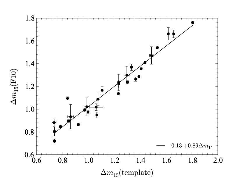
Figure 6: Comparison of the decline rate parameter as measured by F10, $\Delta m_{\mathrm{15}}(B)$ with the value determined through template fitting. The solid line shows the best linear fit to the data.

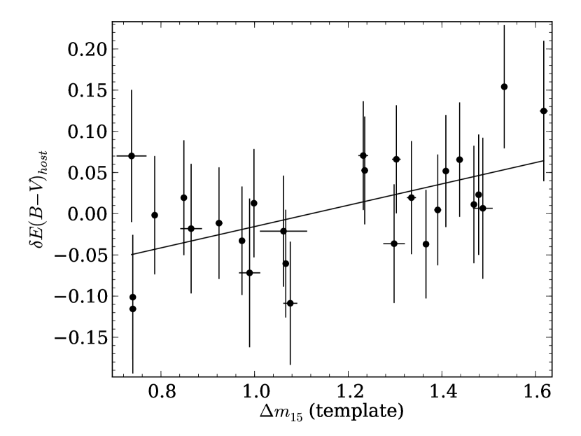
Figure 17: Difference between the $E(B-V)$ values derived by F10 and those determined through MCMC modeling excluding the red sample as a function of $\Delta m_{\mathrm{15}}$. The solid line is a fit to the trend: $E(B-V)_{MCMC}-E(B-V)_{F10}=-0.15+0.13\Delta m_{\mathrm{15}}$.

First, we can use the “unreddened” subsample from F10 and assign these SNe zero extinction, with some intrinsic scatter $\sigma_{c}$ and the rest are allowed to have non-zero extinction. We shall refer to this as the “blue prior”. Second, we can forget the “unreddened” sample and assume a prior for $E(B-V)$ peaked at zero, with an intrinsic scatter of $\sigma_{c}$ and with a tail to higher extinctions with characteristic length $\tau$ . This is motivated by the work of Hatano et al. (1998), who modeled the likely extinction disribution in host disk galaxies, and the later analysis of Jha et al. (2007) who found that the colors of SNe Ia follow such a distribution (see Figure 6 of Jha et al. (2007) and Figure 17 of Kessler et al. (2009)). We shall refer to this as the “Jha prior”. Assigning this prior to each SN Ia, the MCMC method should converge such that $E(B-V)$ = 0 for the bluest SNe.

Using these two MCMC models, we fit the calibration parameters once with all normal SNe Ia ($\Delta m_{\mathrm{15}}<1.7$) in the sample then again with the two very red SNe (SN 2005A and SN 2006X) removed. This gives us 4 sets of calibration parameters that allow us determine the systematic effects of the red SNe and of the assumed extinction prior.

LABEL:15 compares the values of $E(B-V)$ derived through the MCMC model using the blue prior to those of F10. There is a good deal of scatter somewhat above what would be expected from the errors alone. However, there is a clear trend that the most reddened objects in F10 are the most reddened objects in the MCMC analysis. The excess scatter is due to a systematic trend with $\Delta m_{\mathrm{15}}$ which we describe below.

The left panel of LABEL:16 shows the difference between the values of $E(B-V)$ derived using the two different extinction priors. As one can clearly see, there is no large systematic difference between the two sets. However, whether we include the two red SNe does have a systematic effect, as can be seen in the right panel of LABEL:16, where we use the same extinction prior. This is in agreement with the results of F10, who found that the two red SNe Ia seem to follow a different reddening law than the bluer SNe Ia. Due to their very red colors, SN 2005A and SN 2006X have a large pull on the values of $R^{BV}_{X}$ in equation (6), favoring smaller values. The MCMC simulation then responds by modifying the values of $E(B-V)$ in such a way that the average color correction is preserved: the redder objects have more color excess to compensate the smaller $R^{BV}_{X}$. This can also be seen in Table 5 where we list the wavelength-independent calibration parameters. The red SNe Ia drive $R_{V}$ to lower values, however the bluer SNe Ia prefer a larger $R_{V}$. As a consequence, including the red SNe also increases the derived intrinsic dispersion in the SNe Ia.

The extinction prior and inclusion of the red SNe Ia has a smaller effect on the filter-specific calibration parameters, which all agree to within the statistical errors. A marked difference between these results and those of F10 is the difference in the slopes, $b_{x}$. In F10, the slopes were systematically higher and became smaller with redder filter. The reason for the smaller slopes is due to two systematic effects. First, as shown earlier in LABEL:6, there is a systematic difference between $\Delta m_{\mathrm{15}}(B)$ and $\Delta m_{\mathrm{15}}$ such that $\Delta m_{\mathrm{15}}(B)\sim 0.9\Delta m_{\mathrm{15}}$, and so the $\Delta m_{\mathrm{15}}$ correction factor, $b_{x}$, will tend to be smaller. Second, there is also a systematic difference between our estimates of $E(B-V)$ and those from F10 as a function of $\Delta m_{\mathrm{15}}$. These are shown in LABEL:17 and clearly indicate a systematic difference correlated with $\Delta m_{\mathrm{15}}$ in the sense that larger $\Delta m_{\mathrm{15}}$ produces larger $E(B-V)$ than estimated in F10. In this way, the $\Delta m_{\mathrm{15}}$ dependence is partly absorbed into the $E(B-V)$ term of equation (6), resulting again in smaller $b_{x}$. The reason for this systematic difference in $E(B-V)$ is that we have excluded SN 2006gt from our sample of “unreddened” SNe Ia. This one object had a relatively large $\Delta m_{\mathrm{15}}\sim 1.7$ and very red colors ($B-V\sim 0.2$) and therefore tended to make the SNe Ia intrinsically redder for larger $\Delta m_{\mathrm{15}}$.

The calibration parameters for the Color Excess model are given in Table 6. For each parameter we show values derived with and without the red SNe, and also with the two different $E(B-V)$ priors. Due to the fact that there does seem to be something different about including these extremely red events, we recommend using the calibration which was derived without them. This subsample most closely resembles calibration 6 in Table 9 of F10. The fits to the absolute magnitude- $\Delta m_{\mathrm{15}}$ relation for this subsample are shown in LABEL:18.

4.4 Systematic Error Budget

While fitting light curves with any least-squares method supplies us with reliable statistical errors on the light-curve parameters, care must be taken when computing the error in the absolute distance to a single galaxy hosting an individual (or group of) SN Ia (Schweizer et al., 2008; Stritzinger et al., 2010). There are 4 kinds of systematics that need to be taken into account in order to report accurate error estimates on SN Ia-derived distances:

1. The Hubble law was used to determine the absolute magnitudes of the SN Ia sample, and so the assumed Hubble constant ($H_{0}=72~{}{\rm km}\cdot{\rm s}^{-1}\cdot{\rm Mpc}^{-1}$) sets the scale of all derived distances. Currently, there has been a marked improvement in the error budget for $H_{0}$, having been reduced from $\pm 10$% (Freedman et al., 2001) to $\pm 5$% (Riess et al., 2009; Freedman & Madore, 2010). Any further improvement of this error in $H_{0}$ will directly benefit SN Ia-derived distances.

2. The uncertainties the calibration parameters $M_{X}$, $b_{X}$, and $R_{V}$ introduce systematic errors in the distance. The magnitude of these errors will depend on which filters are used and their relative weights. There are also significant covariances between the calibration parameters, particularly between the $M_{X}$ and $R_{V}$. For this reason, computing the systematic error is best done using Monte-Carlo techniques, drawing from the posterior probability distribution output by the MCMC run. We have included routines to do this in SNooPy.

3. After the $\Delta m_{\mathrm{15}}$ and color-dependent corrections have been performed, there remains an intrinsic dispersion in the SN Ia distances that is not explained by measurement error. This extra dispersion $\sigma_{SN}$ should be added in quadrature to the other systematic errors for a single event. However, if multiple events are used to determine the distance to a galaxy (see e.g., Stritzinger et al. (2010)), then these errors should reduce by $\sqrt{N}$.

4. If the SN Ia was observed in a photometric system different than the CSP, or if the redshift of the object is sufficiently large to require cross-band K-corrections, then the errors in the zero-points of each filter must be included. For the CSP filters, this amounts to approximately 0.02 mag in the distance modulus (1% in distance). These must be added in quadrature with the errors of any other photometric system used to observe the SN Ia.

Which of these systematics should be included depends greatly on the application. For instance, when using SNe Ia for cosmology, the error in the Hubble constant drops out, since we are only interested in the relative distances between the SN Ia. However, if the absolute distance to a galaxy is the quantity of interest, then all these errors must be taken into account.

4.5 Hubble Diagram and Host Distances

Now that we have a calibration from the low-$z$ sample, we can fit the full $uBVgriYJH$ light curves of all 34 SNe in our sample (we do not use the two SN Ia that have $\Delta m_{\mathrm{15}}>1.7$). To illustrate this, we construct a Hubble diagram using the measured CMB velocities from NED, and the distance moduli yielded by the $E(B-V)$ model with the calibration parameters derived in §4.3.2. Table 2 lists the parameters derived from the SNooPy fits, the last column showing the distance modulii. We choose the calibration for which we excluded the two red SNe Ia and used the blue subsample to anchor the colors, as this contains the fewest nuisance parameters. The resulting Hubble diagram is shown in the top panel of LABEL:19. The points are the individual SNe Ia. The solid line shows the standard cosmology ($H_{o}=72{\rm km}\cdot{\rm s}^{-1}\cdot{\rm Mpc}^{-1}$, $\Omega_{m}=0.28$, $\Omega_{\Lambda}=0.72$) used in F10 while the dashed line shows the simple Hubble law $v=H_{o}D$ for comparison. The solid line is not a fit to the data, as this would be completely circular, since the cosmology was assumed to derive the calibration parameters in the first place. The residuals between the SNooPy-derived distances and standard cosmology are shown in the bottom panel of LABEL:19. As expected, the dispersion increases at lower redshifts, where peculiar velocities exceed the Hubble flow velocity. SN 2006X, in particular, stands out at the low-$z$ end of the Hubble diagram. Its residual is larger due to peculiar velocities, but also because we chose the calibration that excluded it and SN 2005A.

While the lowest-redshift SNe Ia ($z<0.01$) cannot be used to calibrate the Tripp or Color Excess relations, nor can they be used to constrain cosmological models, they are still of interest, as they serve as distance indicators to their host galaxies. As such, SNe Ia can serve as useful standard candles to those galaxies that lie in the “gap” between the furthest measured Cepheids and the distance at which the Hubble flow can be considered to be in excess of any expected peculiar velocities. The SNe Ia (and hosts) that have $z<0.01$ are: SN 2005W (NGC 691), SN 2005am (NGC 2811), SN 2005ke (NGC 1371), SN 2006D (MRK 1337), SN 2006mr (Fornax A), and SN 2007af (NGC 5584).

Of these low-$z$ objects, we can determine distances to those for which $\Delta m_{\mathrm{15}}<1.7$. According to NED, NGC 691 has a Tully-Fisher distance of $\mu=32.71\pm 0.40$ mag (Tully et al., 2008). This compares very well with the SNooPy distances of $\mu=32.73\pm 0.13$ mag using SN 2005W. We could not find a velocity-independent distance for NGC 2811 with which to compare our distance of $\mu=32.33\pm 0.18$ mag, however it is reasonably close to the Virgo-corrected $\mu=32.52\pm 0.15$ mag reported by NED. The distance to MRK 1337 has been measured by other authors (Mandel et al., 2009; Wood-Vasey et al., 2008) who derive a distance of $\mu=32.72\pm 0.06$ mag using NIR observations of SN 2006D. We therefore contribute an independent distance of $\mu=32.71\pm 0.14$ to SN 2006D, which agrees very well. The treatment of the distance of Fornax A using SNooPy is discussed in a separate, dedicated paper (Stritzinger et al., 2010). Finally, the distance to NGC 5584 has a Tully-Fisher distance of $\mu=31.48\pm 0.52$ mag (Tully et al., 2008). While quite different from the SNooPy distance of $\mu=31.90\pm 0.11$, it is well within the error and agrees well with the Virgo-corrected $\mu=32.10\pm 0.15$ mag distance.

5 Conclusions

In this paper, we have presented SNooPy, a SN Ia light-curve template generator and method appropriate for determining distances to nearby galaxies. These templates have also been used to interpolate the peak rest-frame $i$-band fluxes of a sample of high-$z$ SNe, allowing the first $i$-band Hubble diagram out to redshifts of 0.7. To our knowledge, SNooPy is the only fitter that can simultaneously fit SN Ia light curves from $u$ band all the way to the NIR $H$ band. It therefore has the advantage of a very large wavelength coverage.

This purpose of this paper was mainly to present the methodology used by the CSP to fit light-curves and provide a calibration that is more consistent with the way SNooPy determines distances. The details of the light-curve templates and the calibration parameters will no doubt change as more SNe Ia are added to the low-z sample. In particular, we caution the reader that the small number (2) of significantly reddened objects leads to significantly different results when they are included in the calibration. We therefore recommend that these calibrations not be used and present them only to illustrate the effects of including these highly reddened SNe Ia. Indeed, objects such as these would be selected against in high-redshift surveys. The mere fact that the CSP SNe were selected in a very different way (targeted search) than the blind high-z surveys will lead to some systematic biases. These systematics will be further investigated when larger numbers of CSP SNe Ia are available.

The construction of the light-curve templates, which represent some average behavior of a sample of SNe Ia, has also revealed that at longer wavelengths, there is a marked increase in the SN-to-SN variation in light-curve behavior, even at a given decline rate. Tentatively, it also seems that the peak of the light curves show the least dispersion as standardizable candles. This poses a challenge for the observer, as SN events are typically “triggered” in the optical bands and the light curves peak earlier in the NIR. It is therefore often necessary to use template light curves to extrapolate the peak magnitude. On one hand, the increased dispersion in light-curve behavior will make this extrapolation more uncertain in the NIR. At the same time, these variations hint that another light-curve parameter might be at work and that this parameter may be correlated with residuals in the Hubble diagram. If this turns out to be the case, the inclusion of NIR light curves will deliver a significant advantage to SN Ia cosmology.

We have also presented a least-squares method to determine distances to SN Ia by simultaneously fitting any combination of $uBVgriYJH$ photometry. This method gives distance moduli with an rms scatter of about 0.06 magnitudes (3% in distance). However, added to this small dispersion are the various systematic errors. These include the use of the Hubble constant to determine the distances to the calibrating sample, the formal uncertainties in the calibration parameters, the intrinsic dispersion in the luminosities of SNe Ia, and errors in the photometric zero-points.

Reduction of these systematic errors will improve the use of SNe Ia as standard candles. There is work being done to reduce the error in the Hubble constant to $\pm 2\%$ (Freedman & Madore, 2010), which will, by extension, greatly improve SN Ia distances. In this paper, we used approximately one third of the CSP low-$z$ sample. Including the entire sample will reduce the errors in the calibrating constants, thereby reducing the systematic errors. The intrinsic dispersion in the SN Ia luminosities, $\sigma_{SN}$, will not improve with a larger calibrating sample. Lastly, the CSP is currently working on directly scanning the filter, CCD and telescope throughputs in order to reduce the uncertainty in the photometric zero-points as well as improving S- and K-corrections.

Using SNooPy, we have fit the distances of several SNe Ia that are not in the Hubble flow. Comparison of these distances with other methods gives good agreement in general, particularly when comparing the same SN Ia distance to SN 2006D (MRK 1337).

Appendix A CSP Photometry

The CSP photometry has been published in natural magnitudes in order to simplify their incorporation in other photometric systems. Here, we briefly explain the natural system for the benefit of those who would wish to combine our data with theirs.

Because the filters used on a particular instrument and telescope are not perfect matches to the filters used to establish a photometric system of standards, such as those presented in Landolt (1992) and Smith et al. (2002), color terms are needed to convert observed instrumental magnitudes to standard magnitudes. This is typically done by observing a sequence of standard stars with a spread in colors and comparing the instrumental magnitudes to the published standard magnitudes, fitting a formula of the type $A^{\prime}=A+ct_{A}\left(B-C\right)$ where $A^{\prime}$ is the magnitude in filter $A$ of a standard star in the standard system, $A$, $B$, and $C$ are instrumental magnitudes through filters $A$, $B$, and $C$, and $ct_{A}$ is the color term for filter $A$. The CSP has determined their color terms and published them in Hamuy et al (2006), which we reproduce here for convenience:

$$B^{\prime} = B+0.060(0.013)\left(B-V\right)$$

$$V^{\prime} = V-0.057(0.013)\left(V-i\right)$$

$$u^{\prime} = u+0.051(0.017)\left(u-g\right)$$

$$g^{\prime} = g-0.017(0.009)\left(g-r\right)$$

$$r^{\prime} = r-0.019(0.017)\left(r-i\right)$$

$$i^{\prime} = i-0.007(0.017)\left(r-i\right)$$

The problem is that these color terms are determined using stellar SEDs. SN Ia, in contrast, have broad absorption features that vary with time, and so applying these equations to the instrumental SN Ia to obtain standard magnitudes is not valid. This is the reason that different telescopes observing the same SN Ia end up with significantly different magnitudes, even though both data sets have been converted to a “standard system”. The solution to this problem is to publish natural photometry along with the filter functions used to make the observations. This is done in the following manner.

First, the equations above are used in reverse to convert the standard magnitudes of Smith et al. (2002) and Landolt (1992) into the CSP natural system. Then these new magnitudes along with observations of the standard stars are used to determine the zero-points for the observations of the SN Ia. In this way, the natural system magnitude through filter A are equivalent to

$$m_{A}=-2.5\log_{10}\left(\frac{\int F_{A}\left(\lambda\right)\Phi_{SN}\left(\lambda\right)\lambda d\lambda}{\int F_{A}\left(\lambda\right)\Phi_{std}\left(\lambda\right)\lambda d\lambda}\right)$$ (A1)

where $F_{A}$ is the filter function (including filter transmission, CCD and telescope response functions, and atmospheric extinction) that corresponds to the telescope that actually made the observations, $\Phi_{SN}$ is the SED of the SN Ia that was observed, and $\Phi_{std}$ is an average SED of the spectral standards used to determine the zero-point. If another telescope observes the same event through a different filter B and the magnitudes are published in its standard system, then an S-correction is simple to determine:

$$S_{BA}\left(t\right)=-2.5\log_{10}\left(\frac{\int F_{A}\left(\lambda\right)\Phi_{SN}\left(\lambda\right)\lambda d\lambda\times\int F_{B}\left(\lambda\right)\Phi_{std}\left(\lambda\right)\lambda d\lambda}{\int F_{B}\left(\lambda\right)\Phi_{SN}\left(\lambda\right)\lambda d\lambda\times\int F_{A}\left(\lambda\right)\Phi_{std}\left(\lambda\right)\lambda d\lambda}\right)$$ (A2)

where $S_{BA}\left(t\right)$ is an S-correction that converts a magnitude from system B into system A: $m_{A}\left(t\right)=m_{B}\left(t\right)+S_{BA}\left(t\right)$.

SNooPy can perform this transformation automatically by using the Hsiao et al. (2007) SED templates if 1) the input photometry is in a natural system like that described above, and 2) the filter functions of the observed photometric system are supplied. In effect, when both systems are natural, then the S-correction can be considered to be a cross-band K-correction at low redshift.

Appendix B MCMC Modeling

The use of Markov-Chain Monte-Carlo (MCMC) simulations to model data is rapidly growing in popularity in the astronomical community. It has many advantages over the more commonly used $\chi^{2}$ analysis. Most importantly, it allows one to use more realistic statistical models for the data and priors, rather than assuming all errors are normally distributed. Second, the result of the MCMC simulation is a set of parameters drawn from the posterior probability distribution, from which one can easily determine expectation values, modes, variances and co-variances of the parameters of interest.

Readers who are unfamiliar with MCMC may wish to read the pymc documentation. While not mathematically rigorous, it provides an excellent overview of the more technical aspects of the method and its terminology. Pymc is a Python module that greatly simplifies the task of setting up and running MCMC simulations and was used to run the simulations in this paper. The code defining the statistical model is available at the CSP website.

MCMC is a method based on Bayesian statistics. Bayes’ theorem states that the probability distribution of the parameters $\theta$ of a model, given the observed data $D$, is given by

$$p\left(\theta|D\right)=\frac{p\left(D|\theta\right)p\left(\theta\right)}{p\left(D\right)}$$ (B1)

where $p\left(D|\theta\right)$ is the probability that we observe $D$, given $\theta$, $p\left(\theta\right)$ is the prior distribution of the parameters, and $p\left(D\right)=\int p\left(D|\theta\right)p\left(\theta\right)d\theta$. The functional form of $p\left(D|\theta\right)$ is straightforward, as is $p\left(\theta\right)$. However, the set of parameters $\theta$ will likely contain nuisance parameters over which we wish to marginalize. Performing integrals of the right-hand side of equation (B1) analytically can only be done for the simplest PDFs and priors. Assuming normal distributions, for instance, leads to the well-known $\chi^{2}$ statistic and the method of least squares. For anything more complex, one must numerically integrate equation (B1) to marginalize, compute expectation values, etc.

Markov chain Monte-Carlo is a method for dealing with the situation where equation (B1) cannot be integrated analytically. The method works by creating a Markov Chain of parameter states $\theta_{i}$. Markov Chains have the property that the state $\theta_{i+1}$ depends only on the previous state $\theta_{i}$. The transition from state $\theta_{i}\rightarrow\theta_{i+1}$ is done in a probabilistic way using equation (B1), hence the use of Monte-Carlo in the method’s name. The Markov chain can therefore be thought of as a quasi-random walk through parameter space. The exact details of how the transition is done depends on the MCMC method used. Two popular algorithms are Gibbs sampling and the Metropolis-Hastings algorithm. Regardless of the method, it can be shown that after a certain number of transitions, called burn-in, the Markov chain will become stationary. From that point on, the distribution of states in the Markov chain is equal to $p\left(\theta|D\right)$. In other words, the states in the Markov chain can be considered as random draws from $p\left(\theta|D\right)$. One can therefore use the Markov chain to infer the posterior probability distribution of all the parameters of interest. For this paper, we use the Metropolis-Hastings algorithm.

In order to use the MCMC method, one must construct a probabilistic process that relates the data to the model and specifies any priors $p\left(\theta\right)$. From this, pymc can compute the likelihood. We consider two models, one for the Tripp method and one for the Color Excess method. The Tripp method, being simply linear regression, is the simplest and we describe it first. We then describe the Color Excess model, which has more complicated priors.

B.1 Tripp Model

Given three filters $XYZ$, the data consist of the 3 magnitudes at maximum $m_{x}$, $m_{y}$ and $m_{z}$, the decline-rate $\Delta m_{\mathrm{15}}$, and the redshift $z$. We wish to fit the following model

$$m_{x}^{\prime}=M_{x}^{yz}+b_{x}^{yz}\left(\Delta^{\prime}m_{15}-1.1\right)+R_{x}^{yz}\left(m_{y}^{\prime}-m_{z}^{\prime}\right)+\mu\left(z^{\prime}\right)$$ (B2)

solving for the calibration parameters $M_{x}^{yz}$, $b_{x}^{yz}$, and $R_{x}^{yz}$. The primes in this equation denote “true” values, in order to distinguish them from observed values. The “true” values are nuisance parameters and will be marginalized. We assume that the observables are statistically related to their “true” values through a normal distribution:

$$\left[m_{x},m_{y,}m_{z},\Delta m_{\mathrm{15}},z\right]\sim N_{5}\left(\left[m_{x}^{\prime},m_{y,}^{\prime}m_{z}^{\prime},\Delta m_{\mathrm{15}}^{\prime},z^{\prime}\right],C\right)$$ (B3)

where $N_{5}$ is a 5-dimensional multivariate normal distribution and $C$ is the covariance matrix. The covariances between the light-curve parameters are provided by the least-squares fitting. The value of $m_{x}^{\prime}$ in equation (B3) is given by equation (B2). We also add an extra term $\sigma_{SN}^{2}$ to the $(m_{x},m_{x})$ term of the covariance matrix $C$ that represents any intrinsic scatter in the luminosity of SNe Ia. We leave this as a free parameter and so its value will be determined along with the calibration parameters. Finally, we assign the following priors to the calibration parameters:

$$M_{x}^{yz} \sim U(-\infty,\infty)$$ (B4)

$$b_{x}^{YX} \sim U(-\infty,\infty)$$

$$R_{x}^{yz} \sim U(-\infty,\infty)$$

$$\sigma_{SN} \sim U(0,\infty)$$

where $U(x,y)$ is a uniform prior between $x$ and $y$. This completes the statistical model. The parameters consist of the set $\theta=\left\{M_{x}^{yz},b_{x}^{yz},R_{x}^{yz},\sigma_{SN},m_{x,i}^{\prime},m_{y,i}^{\prime},m_{z,i}^{\prime},\Delta m_{\mathrm{15}}^{\prime},z^{\prime}\right\}$ and the probability of any state $\theta_{i}$ can be computed through equations (B2) to (B4). The Metropolis-Hastings algorithm can then construct a Markov Chain from which we can infer the PPD of all variables of interest.

B.2 Color Excess Model

This model is similar to the Tripp model. In this case, however, we fit all the filters simultaneously. Our data therefore consists of all 9 magnitudes at maximum, $m_{x_{j}}$, the decline-rates, $\Delta m_{\mathrm{15}}$, and the redshifts, $z$. We assume the errors in the observables are once again normally distributed:

$$\left[m_{x_{j}},\Delta m_{\mathrm{15}},z\right]\sim N_{11}\ \left(\left[m_{x_{j}}^{\prime},\Delta m_{\mathrm{15}}^{\prime},z^{\prime}\right],C\right),$$ (B5)

where now the $m_{x_{j}}^{\prime}$ are given by

$$m_{x_{j}}^{\prime}=M_{x_{j}}+b_{x_{j}}\left(\Delta^{\prime}m_{15}-1.1\right)+R_{x_{j}}^{BV}\left(R_{V}\right)E(B-V)+\mu\left(z^{\prime}\right).$$ (B6)

As discussed in §4.1, we treat the color excesses $E(B-V)$ as free parameters. We use two different priors on the values of $E(B-V)$. First, we use the “unreddened” subsample from F10 and assign these SNe a Gaussian prior with zero mean extinction and some unknown scatter $\sigma_{c}$. The other SNe are then assigned a composite prior:

$$E(B-V)\sim\left\{\begin{array}[]{c}N(0,\sigma_{c}),\;E(B-V)<0\\ U(0,\infty),\;E(B-V)>0\end{array}\right.$$ (B7)

where $N\left(0,\sigma_{c}\right)$ is a normal distribution with zero mean and standard deviation $\sigma_{c}$. In this way, the “unreddened” SNe anchor the values of $E(B-V)$ and any SN with colors redder than this sample will have $E(B-V)>0$. Any SNe with significantly bluer colors will have $E(B-V)<0$ and cause $\sigma_{c}$ to be larger.

Second, we can avoid using an unreddened sample and instead use a prior for all the SN Ia that penalizes high values of $E(B-V)$. In this case, we use the prior from Jha et al. (2007), which corresponds to the convolution of a normal distribution $N(0,\sigma_{c})$ with an exponential tail $\exp(-E(B-V)/\tau)$. We leave the variables $\sigma_{c}$ and $\tau$ as nuisance variables to be determined during the MCMC run. In this way, the model will search for a “blue edge” in the color distribution of the SNe Ia. The bluest SNe will determine the intrinsic colors and scatter. The redder SNe will set the scale length of the exponential tail, $\tau$.

Our parameter set now contains 19 calibration parameters: 9 absolute magnitudes, $M_{x_{j}}$, 9 slopes $b_{x_{j}}$, and the reddening law $R_{V}$. Added to this are the intrinsic scatter, $\sigma_{SN}$, the intrinsic color scatter $\sigma_{c}$, the exponential tail scale length $\tau$ (for the Jha prior), the $N$ values of $E(B-V)_{i}$, and all the “true” values of the observables.

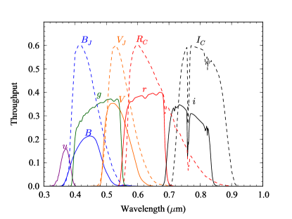
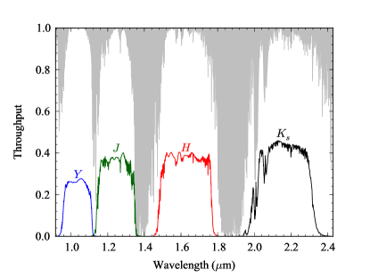
Figure 1: The CSP filter band-passes. Left: the optical filter set $uBVgri$ are plotted as solid lines while the Johnson $BV$ and Cousins $RI$ are plotted as dashed lines for comparison (Stritzinger et al., 2005). Right: the NIR filter set $YJHK_{s}$ are plotted as solid lines and the atmospheric absorption at LCO is plotted as the gray region.

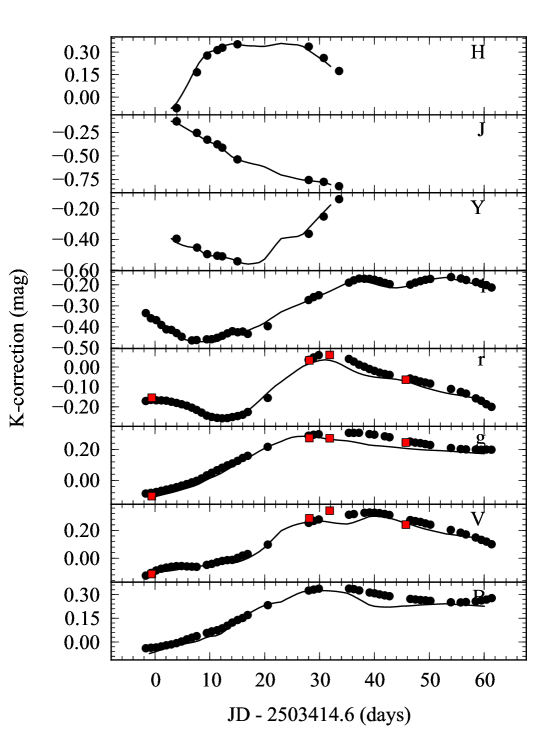
Figure 2: Example K-corrections for SN 2005ag, one of the highest redshift SN Ia in our sample. The K-corrections are computed in 3 ways: (1) using the unmodified Hsiao et al. (2007) SED (lines), (2) warping the Hsiao et al. (2007) SED to match the observed colors (round points), and (3) using the observed spectrum of SN 2005ag (red squares).

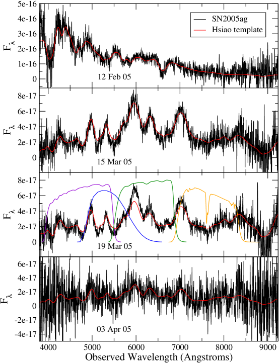
Figure 3: Four spectra of SN 2005ag taking by the CSP (black lines) with the corresponding SEDs from Hsiao et al. (2007) (red lines). The date of observation is labeled in the panels. The colored lines in the 3rd panel are the CSP filter functions: $g$ (blue), $r$ (yellow), $i$ (orange), and $V$ (green).

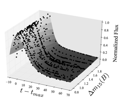
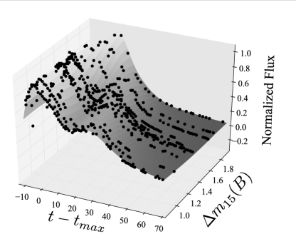
Figure 4: The sparsely sampled 2D surface defined by the training set of SN Ia. The three axes consist of (1) $t_{min}\left(B\right)$, (2) the decline rate, $\Delta m_{\mathrm{15}}$, and (3) the flux normalized to the peak flux. Two filters are shown: $B$ band (left) and $i$ band (right).

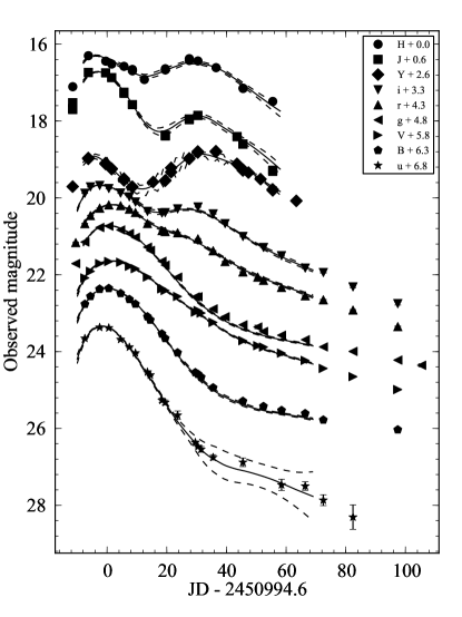
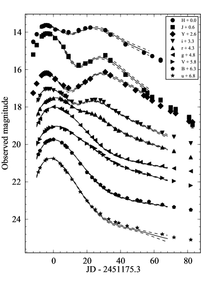
Figure 5: Sample light curve fits using SNooPy for two SN Ia: SN 2006et (left) and SN 2007af (right). The data points are offset by the amount indicated in the legends for clarity. The solid lines are fits to the photometry, the dashed lines are the 1-$\sigma$ template errors.

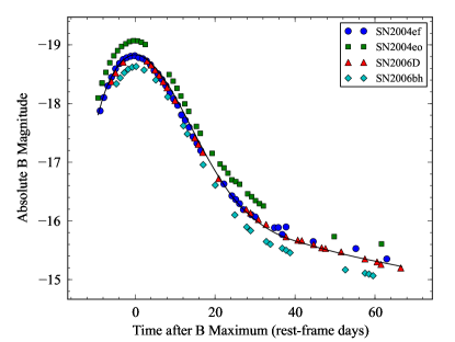
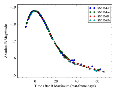
Figure 7: Absolute magnitude $B$-band light curves for four SNe Ia with similar $\Delta m_{\mathrm{15}}$: SN 2004ef ($\Delta m_{\mathrm{15}}=1.36$), SN 2004eo ($\Delta m_{\mathrm{15}}=1.38$), SN 2006D ($\Delta m_{\mathrm{15}}=1.38$), and SN 2006bh ($\Delta m_{\mathrm{15}}=1.43$). Left: the distances are computed using a Virgo-corrected velocity and Hubble constant of $72\ {\rm km}\cdot{\rm s}^{-1}\cdot{\rm Mpc}^{-1}$. Right: the light curves are shifted such that the $B$-maxima agree. The solid lines are SNooPy $B$-band templates for $\Delta m_{\mathrm{15}}=1.4$.

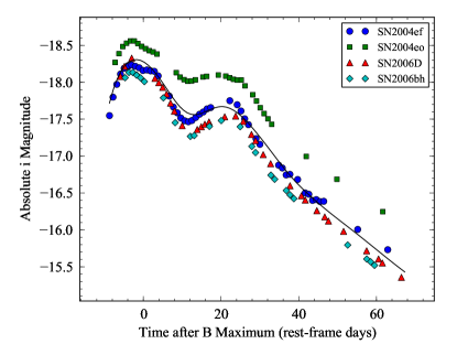
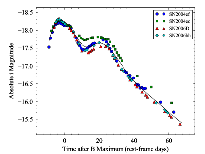
Figure 8: Absolute magnitude $i$-band light curves for the same SNe as in LABEL:7. The distances in the left panel and offsets in right panel are the same as those used in LABEL:7. The solid lines are SNooPy $i$-band templates for $\Delta m_{\mathrm{15}}=1.4$.

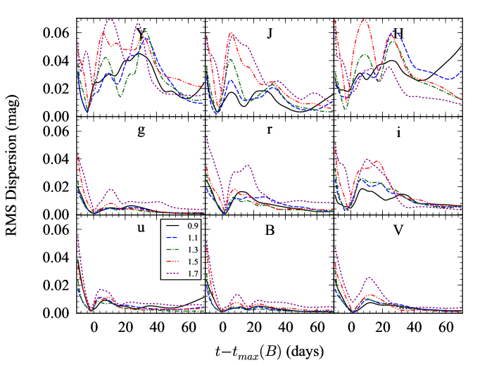
Figure 9: Results of a bootstrap simulation on the dispersion in the light-curve templates due to intrinsic variations from supernova to supernova. Each panel represents a separate CSP filter and the different lines represent different values of $\Delta m_{\mathrm{15}}$. Each line shows the rms dispersion of the templates as a function of time since $B$-maximum.

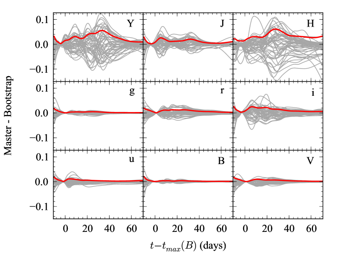
Figure 10: Same as LABEL:9, but for a specific value of $\Delta m_{\mathrm{15}}=1.1$. The grey lines represent the individual bootstrap realizations. The red line represents the rms of all the realizations.

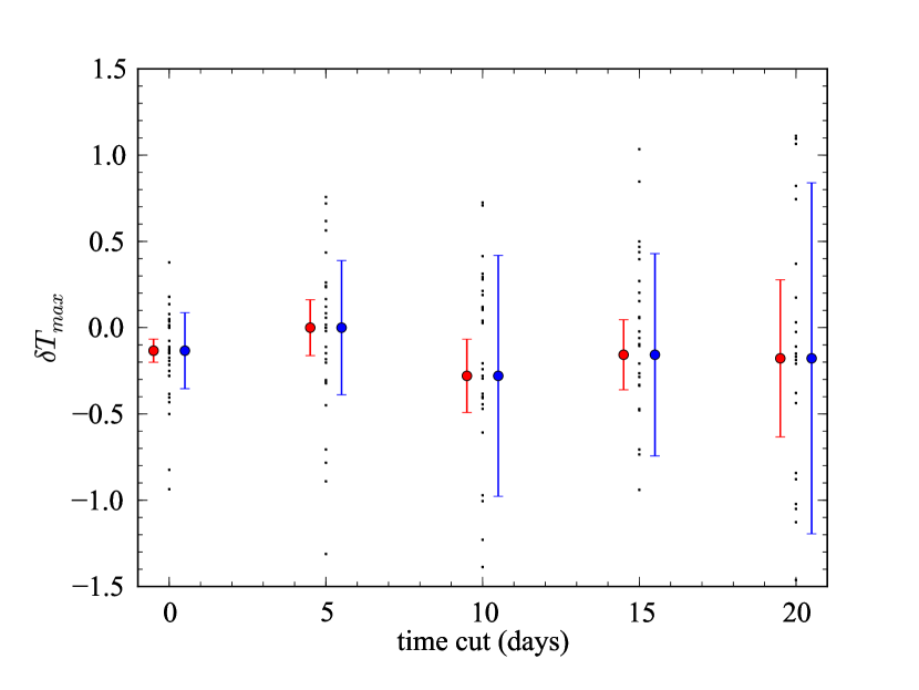
Figure 11: Errors in the value of $t_{max}$ as a function of the time of earliest observation ($t_{cut}$). Each SN Ia is plotted as a black dot. The blue circles and error bars to the right of each set of dots correspond to the median and median absolute deviation, respectively. The red circles and error bars to the left of each set shows the weighed mean deviation after the least-squares error in $t_{max}$ has been removed.

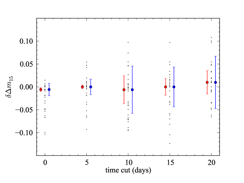
Figure 12: Same as LABEL:11, but for errors in $\Delta m_{\mathrm{15}}$.

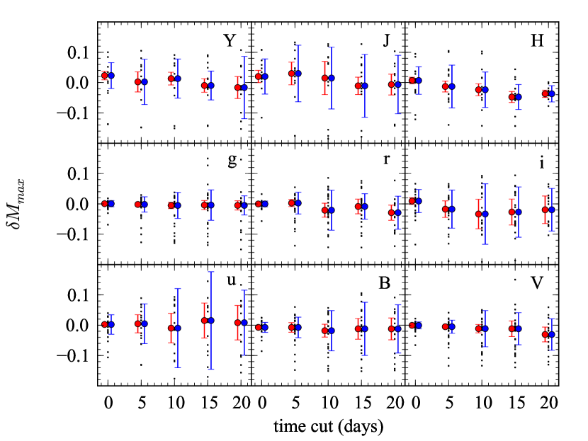
Figure 13: Same as LABEL:11, but for errors in apparent maximum magnitude. Each panel represents a different filter.

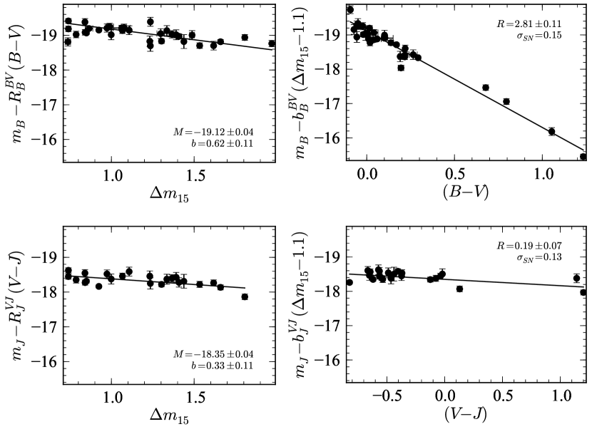
Figure 14: Tripp relation derived from MCMC simulation for two filter combinations. The first row shows filter $B$ corrected by pseudo-color $B_{max}-V_{max}$. The second row shows filter $J$ corrected by pseudo-color $V_{max}-J_{max}$. The left panels show the absolute magnitudes, corrected for color, while the right-hand panels show the absolute magnitudes corrected for $\Delta m_{\mathrm{15}}$. All SNe with redshifts greater than 0.01 are included in the fit. The fit results are labeled.

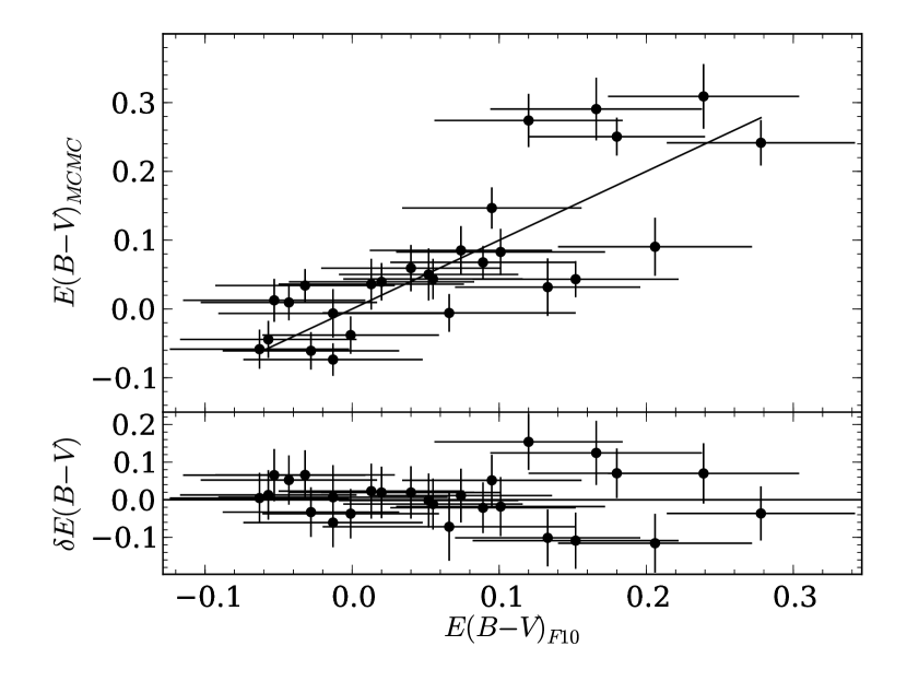
Figure 15: Comparison of values of $E(B-V)$ derived by F10 and determined by the MCMC blue prior model, excluding the two red SNe. The solid line indicates $E(B-V)_{F10}=E(B-V)_{MCMC}$ and is not a fit to the data. The bottom panel shows the residuals about the solid line.

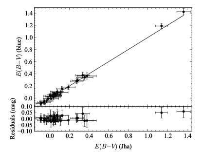
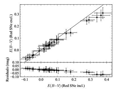
Figure 16: Comparison of values of $E(B-V)$ derived by MCMC. Left: two different priors (the blue prior and Jha prior) are used. Right: two different sub-samples of SN Ia (including and excluding the two red SNe Ia) are used with the blue prior. In both figures, the solid line shows one-to-one correspondence.

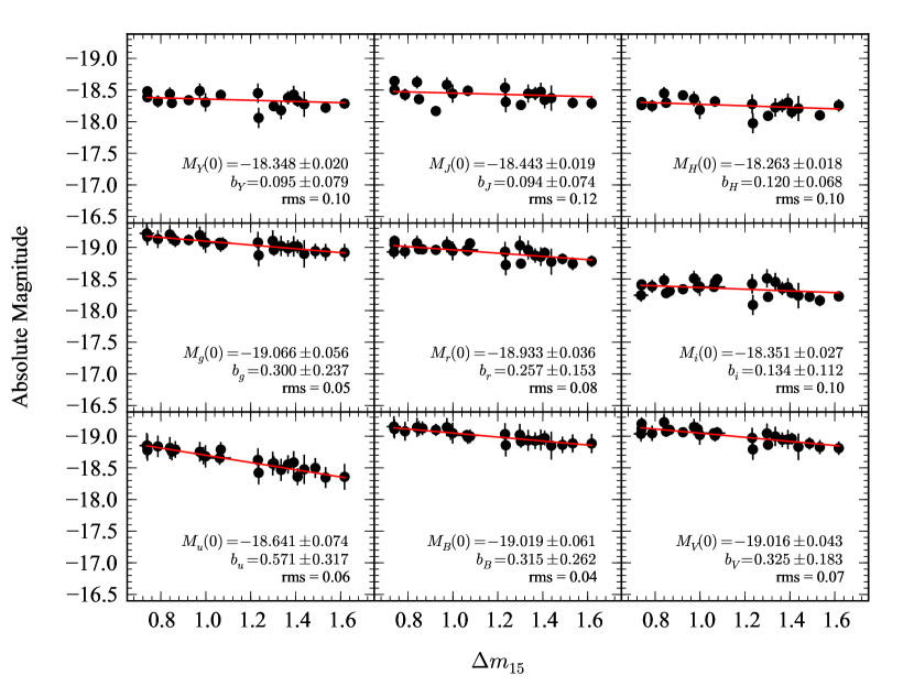
Figure 18: Luminosity-$\Delta m_{\mathrm{15}}$  relation for the Color Excess model derived from MCMC fitting, excluding the two red SNe and three fast-declining SNe. Each panel corresponds one of the CSP filters. The distance moduli from F10 are used to compute the absolute magnitudes of each SN. SNooPy fits are used to compute $\Delta m_{\mathrm{15}}$. The SNe are reddening-corrected using the values of $E(B-V)$ and $R_{V}$ from the MCMC run. The solid lines show the fit to $M_{x}$ and $b_{x}$, which are labeled with uncertainties in each panel.

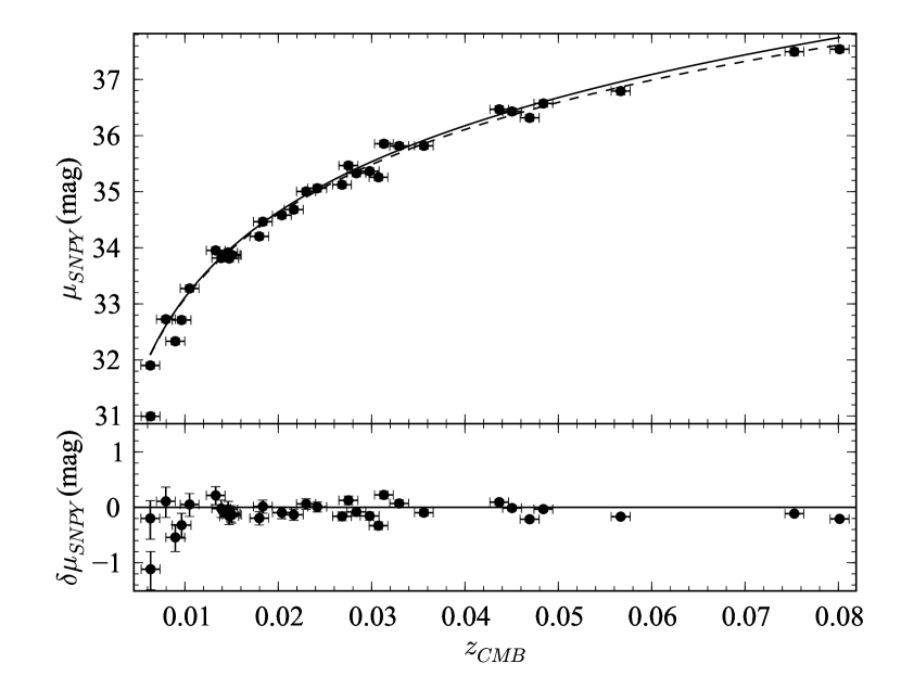
Figure 19: Hubble Diagram constructed from the observed CMB velocities and SNooPy-derived distance moduli, using the full $uBVgriYJH$ filter set. The points are individual SN Ia with error-bars from the fit. The solid line shows the standard cosmology redshift-distance relation, while the dashed line shows the simple Hubble Law for $H_{o}=72\ {\rm km}\cdot{\rm s}^{-1}\cdot{\rm Mpc}^{-1}$.

Table 1: SN Ia used for Calibration and Template Generation

Name	$v_{hel}$	$v_{cmb}$	Host	$t_{0}$	$E(B-V)_{MW}$	Template	Notes
SN	${\rm km\cdot s^{-1}}$	${\rm km\cdot s^{-1}}$		days	mag
(1)	(2)	(3)	(4)	(5)	(6)	(7)	(8)
2004ef	9289	8931	UGC 12158	-8.8	0.06	$uBVgri$
2004eo	4706	4421	NGC 6928	-12.2	0.11	$uBVgriYJH$
2004ey	4733	4388	UGC 11816	-9.0	0.14	$uBVgri$	Blue
2004gc	9203	9214	PGC 017176	5.8	0.21
2004gs	7988	8249	MCG +03-22-020	-3.2	0.03	$uBVgri$
2004gu	13748	14069	FGC 175A	-0.3	0.03
2005A	5738	5502	NGC 0958	-3.9	0.03	$uBVgr$	Red
2005M	6599	6891	NGC 2930	-8.0	0.03	$uBVgriYJH$	Blue
2005W	2665	2385	NGC 0691	-8.0	0.07	$uBVgri$
2005ag	23811	24024	MAPS-NGP O 502 0366176	-1.6	0.04		Blue
2005al	3718	3986	NGC 5304	-0.7	0.05	$uBVgr$	Blue
2005am	2368	2690	NGC 2811	-4.1	0.05	$uBVgri$	Blue
2005be	10500	10673	NPM1G +16.0412	7.5	0.03
2005bg	6921	7247	MCG +03-31-093	1.3	0.03
2005bl	7213	7534	NGC 4070	-5.6	0.03		Fast
2005bo	4166	4504	NGC 4708	-0.3	0.05
2005el	4470	4465	NGC 1819	-7.3	0.11	$uBVgriYJH$	Blue
2005eq	8687	8505	MCG -01-09-006	-3.4	0.07	$BVgrYJH$
2005hc	13772	13503	MCG +00-06-003	-4.7	0.03	$uBVgr$	Blue
2005iq	10206	9879	ESO 538- G 013	-5.4	0.02	$uBVgri$	Blue
2005ir	22892	22570	SDSS J011643.87+004736.9	-2.2	0.03
2005kc	4533	4167	NGC 7311	-10.7	0.13	$uBVgriYJH$
2005ke	1463	1345	NGC 1371	-9.0	0.03	$uBVgriYJH$	Blue,Fast
2005ki	5758	6111	NGC 3332	-9.7	0.03	$uBVgriYJH$	Blue
2005lu	9596	9388	ESO 545- G 038	9.6	0.03
2005na	7891	8044	UGC 03634	-1.9	0.08	$BVgr$
2006D	2556	2892	MRK 1337	-5.9	0.05	$BVgriYJH$	Blue
2006X	1571	1896	NGC 4321	-10.0	0.03	$YJH$	Red
2006ax	5018	5387	NGC 3663	-11.7	0.05	$uBVgriYJH$	Blue
2006bh	3252	3148	NGC 7329	-4.8	0.03	$uBVgriYJH$	Blue
2006eq	14840	14510	2MASX J21283758+0113490	5.3	0.05
2006et	6652	6494	NGC 232	-7.4	0.02	$uBVgriYJH$
2006gt	13422	13093	2MASX J00561810-0137327	-1.3	0.04		Fast
2006mr	1760	1653	NGC 1316	-4.2	0.02	$uBVgriYJH$	Fast
2006py	17357	16993	SDSS J224142.04-000812.9	-1.5	0.06
2007af	1639	1887	NGC 5584	-9.0	0.04	$uBVgriYJH$

Note. — Columns: (1) SN  name; (2) heliocentric radial velocity from the NASA/IPAC Extragalactic Database (NED); (3) radial velocity in the frame of the Cosmic Microwave Background (CMB) from NED; (4) host galaxy name from NED; (5) time of earliest photometric observation relative to $B$-band maximum; (6) Milky Way reddening (Schlegel et al., 1998); (7) list of filters for which this object was used to generate light-curve templates; (8) Notes: “Blue” denotes an unreddened SN  Ia from F10, “Red” denotes a highly-reddened SN Ia from F10, and “Fast” denotes a fast-declining (e.g., SN  1991bg-like) SN Ia.

Table 2: SN Ia Light Curve Parameters

Name	$\Delta m_{15}\left(B\right)$	$\Delta m_{15}$	$t_{max}\left(B\right)$	$t_{max}$	$E(B-V)$	$\mu$
SN	mag	mag	days	days	mag	mag
(1)	(2)	(3)	(4)	(5)	(6)	(7)
2004ef	1.36(0.01)	1.41(0.01)	264.41(0.04)	264.02(0.10)	0.226(0.005)	35.37(0.01)
2004eo	1.38(0.05)	1.33(0.01)	278.84(0.35)	278.25(0.12)	0.131(0.006)	33.81(0.01)
2004ey	0.93(0.01)	1.00(0.01)	304.40(0.10)	304.07(0.10)	-0.035(0.003)	33.92(0.01)
2004gc	…	1.08(0.02)	…	323.55(0.41)	0.188(0.010)	35.26(0.02)
2004gs	1.61(0.04)	1.53(0.01)	356.49(0.08)	355.58(0.12)	0.299(0.005)	35.47(0.01)
2004gu	…	0.74(0.01)	…	361.66(0.22)	0.125(0.008)	36.32(0.01)
2005A	1.12(0.04)	1.11(0.01)	380.33(0.16)	380.00(0.20)	1.083(0.011)	34.46(0.02)
2005M	0.83(0.02)	0.79(0.01)	405.86(0.26)	405.25(0.10)	0.044(0.004)	35.00(0.01)
2005W	1.22(0.06)	1.15(0.02)	412.34(0.04)	412.05(0.12)	0.221(0.004)	32.73(0.01)
2005ag	…	0.92(0.01)	…	413.89(0.17)	0.021(0.005)	37.54(0.01)
2005al	1.16(0.02)	1.24(0.01)	430.28(0.13)	429.95(0.14)	0.014(0.004)	33.95(0.01)
2005am	1.47(0.06)	1.48(0.01)	436.93(0.24)	436.16(0.13)	0.156(0.004)	32.33(0.01)
2005be	…	1.49(0.03)	…	459.91(0.49)	0.029(0.019)	35.82(0.02)
2005bg	…	0.99(0.02)	…	469.80(0.34)	-0.028(0.017)	35.06(0.03)
2005bo	…	1.30(0.02)	…	478.55(0.20)	0.347(0.005)	33.87(0.01)
2005el	1.34(0.01)	1.39(0.01)	647.56(0.03)	646.65(0.11)	-0.005(0.004)	33.88(0.01)
2005eq	0.72(0.04)	0.74(0.01)	654.24(0.36)	653.73(0.15)	0.033(0.004)	35.33(0.01)
2005hc	0.90(0.01)	0.85(0.01)	667.39(0.08)	666.91(0.12)	0.019(0.004)	36.43(0.01)
2005iq	1.25(0.02)	1.30(0.01)	688.14(0.08)	687.48(0.11)	0.022(0.004)	35.81(0.01)
2005ir	…	0.86(0.02)	…	684.35(0.27)	0.050(0.014)	37.50(0.03)
2005kc	1.19(0.02)	1.23(0.01)	698.06(0.19)	697.68(0.11)	0.316(0.005)	33.82(0.01)
2005ke	1.73(0.01)	1.81(0.01)	698.78(0.05)	698.19(0.10)	…	…
2005ki	1.37(0.01)	1.37(0.01)	706.07(0.06)	705.08(0.11)	0.020(0.003)	34.58(0.01)
2005lu	…	0.74(0.04)	…	710.53(0.57)	0.215(0.011)	35.85(0.02)
2005na	0.95(0.04)	1.07(0.01)	740.20(0.34)	740.16(0.15)	-0.018(0.007)	35.12(0.02)
2006D	1.38(0.01)	1.47(0.01)	757.75(0.03)	757.26(0.10)	0.204(0.004)	32.71(0.01)
2006X	1.09(0.02)	0.84(0.01)	786.08(0.27)	785.23(0.15)	1.345(0.012)	30.99(0.02)
2006ax	1.00(0.01)	0.97(0.01)	827.53(0.12)	826.85(0.11)	-0.036(0.004)	34.20(0.01)
2006bh	1.37(0.02)	1.44(0.01)	833.55(0.11)	833.17(0.10)	0.065(0.003)	33.27(0.01)
2006eq	…	1.62(0.01)	…	975.82(0.47)	0.311(0.011)	36.57(0.02)
2006et	0.85(0.03)	0.84(0.01)	993.55(0.36)	-52005.86(0.13)	0.183(0.006)	34.68(0.01)
2006gt	…	1.66(0.01)	…	1002.45(0.17)	0.288(0.011)	36.47(0.02)
2006mr	1.94(0.03)	2.05(0.01)	1050.62(0.10)	1050.35(0.11)	…	…
2006py	…	1.06(0.05)	…	1070.51(0.36)	0.094(0.011)	36.79(0.03)
2007af	1.20(0.03)	1.11(0.01)	1174.78(0.14)	-51825.20(0.10)	0.183(0.003)	31.90(0.00)

Note. — Columns: (1) SN name; (2) decline-rate parameter measured directly from $B$-band light curve (see §3.3); (3) decline-rate parameter derived from SNooPy fits; (4) date of $B$-band maximum measured from $B$-band light curve (${\rm JD}-2453000$); (5) date of $B$-band maximum derived from SNooPy fits; (6) color excess derived from SNooPy fits; (7) distance modulus derived from SNooPy fits for SNe Ia with $\Delta m_{15}<1.7$ and two red SNe Ia excluded.

Table 3: Extrapolation Errors in Light-Curve Parameters

	Time of Earliest Observation
Parameter	0 days	5 days	10 days	15 days	20 days
$t_{max}$	0.07	0.16	0.21	0.21	0.46
$\Delta m_{\mathrm{15}}$	0.00	0.00	0.03	0.03	0.03
$u_{max}$	0.00	0.03	0.05	0.06	0.06
$B_{max}$	0.00	0.02	0.02	0.03	0.04
$V_{max}$	0.00	0.00	0.01	0.03	0.03
$g_{max}$	0.00	0.01	0.01	0.01	0.02
$r_{max}$	0.00	0.01	0.02	0.02	0.02
$i_{max}$	0.01	0.03	0.05	0.05	0.05
$Y_{max}$	0.01	0.03	0.03	0.03	0.04
$J_{max}$	0.02	0.04	0.05	0.05	0.05
$H_{max}$	0.01	0.02	0.02	0.02	0.02

Table 4: Tripp Calibration Parameters

		Red SNe incl.				Red SNe excl.
Filter	Color	$M_{X}^{YZ}$	$b_{X}^{YZ}$	$R_{X}^{YZ}$	$\sigma_{SN}$	$M_{X}^{YZ}$	$b_{X}^{YZ}$	$R_{X}^{YZ}$	$\sigma_{SN}$
$u$	$g-r$	-18.19 (0.05)	0.63 (0.15)	4.1 (0.2)	0.24	-18.22 (0.06)	0.52 (0.18)	3.8 (0.5)	0.23
$u$	$B-V$	-18.72 (0.05)	0.48 (0.12)	4.1 (0.1)	0.19	-18.72 (0.05)	0.62 (0.16)	4.0 (0.4)	0.19
$B$	$B-V$	-19.12 (0.04)	0.62 (0.11)	2.8 (0.1)	0.15	-19.08 (0.04)	0.42 (0.12)	3.0 (0.3)	0.15
$V$	$B-V$	-19.07 (0.04)	0.38 (0.09)	1.8 (0.1)	0.14	-19.08 (0.04)	0.41 (0.12)	2.0 (0.3)	0.15
$g$	$g-r$	-18.80 (0.04)	0.43 (0.11)	2.4 (0.1)	0.18	-18.81 (0.04)	0.35 (0.14)	2.4 (0.4)	0.18
$r$	$g-r$	-18.80 (0.04)	0.43 (0.11)	1.4 (0.1)	0.17	-18.81 (0.04)	0.36 (0.14)	1.4 (0.4)	0.18
$i$	$g-r$	-18.29 (0.04)	0.27 (0.11)	1.1 (0.1)	0.18	-18.28 (0.05)	0.20 (0.15)	1.1 (0.4)	0.19
$Y$	$V-J$	-18.22 (0.03)	0.23 (0.08)	0.3 (0.1)	0.08	-18.26 (0.06)	0.21 (0.09)	0.2 (0.1)	0.04
$J$	$V-J$	-18.35 (0.04)	0.33 (0.11)	0.2 (0.1)	0.13	-18.48 (0.09)	0.38 (0.13)	-0.1 (0.2)	0.09
$H$	$V-J$	-18.19 (0.03)	0.24 (0.08)	0.2 (0.1)	0.07	-18.18 (0.08)	0.20 (0.11)	0.3 (0.2)	0.06

Table 5: Calibration Parameters for the Reddening Model

Case	$R_{V}$	$\sigma_{SN}$	$\sigma_{c}$	$\tau$
Red SNe incl.	1.40 (0.06)	0.08	0.08	…
Red SNe excl.	1.95 (0.16)	0.05	0.07	…
Jha Prior + Red SNe incl.	1.51 (0.07)	0.09	0.10	0.26
Jha Prior + Red SNe excl.	2.64 (0.25)	0.07	0.10	0.08

Table 6: Filter-Specific Calibration Parameters for the Reddening Model

	Red SNe incl.		Red SNe excl.		Jha Prior		Jha Prior + Red SNe excl.
Filter	$M_{0}$	$b$	$M_{0}$	$b$	$M_{0}$	$b$	$M_{0}$	$b$
u	-18.62 (0.08)	0.46 (0.31)	-18.64 (0.08)	0.58 (0.32)	-18.62 (0.16)	0.25 (0.49)	-18.52 (0.11)	0.55 (0.34)
B	-19.02 (0.06)	0.32 (0.24)	-19.02 (0.06)	0.32 (0.26)	-19.03 (0.12)	0.15 (0.39)	-18.92 (0.10)	0.29 (0.29)
V	-19.00 (0.04)	0.32 (0.15)	-19.01 (0.04)	0.33 (0.18)	-19.01 (0.08)	0.21 (0.25)	-18.96 (0.07)	0.30 (0.22)
g	-19.07 (0.05)	0.33 (0.22)	-19.07 (0.06)	0.31 (0.24)	-19.08 (0.11)	0.18 (0.35)	-18.98 (0.09)	0.28 (0.27)
r	-18.92 (0.03)	0.26 (0.12)	-18.93 (0.04)	0.26 (0.15)	-18.94 (0.06)	0.17 (0.20)	-18.89 (0.06)	0.22 (0.19)
i	-18.32 (0.02)	0.11 (0.09)	-18.35 (0.03)	0.14 (0.11)	-18.34 (0.04)	0.03 (0.13)	-18.34 (0.05)	0.09 (0.14)
Y	-18.33 (0.02)	0.10 (0.07)	-18.35 (0.02)	0.10 (0.07)	-18.35 (0.03)	0.07 (0.09)	-18.34 (0.03)	0.06 (0.09)
J	-18.43 (0.02)	0.11 (0.07)	-18.44 (0.02)	0.10 (0.07)	-18.44 (0.03)	0.09 (0.09)	-18.44 (0.03)	0.07 (0.08)
H	-18.25 (0.02)	0.11 (0.07)	-18.26 (0.02)	0.12 (0.06)	-18.26 (0.02)	0.08 (0.08)	-18.26 (0.02)	0.10 (0.07)

References

- Astier et al. (2006) Astier, P., et al. 2006, A&A, 447, 31
- Bohlin (2007) Bohlin, R. C. 2007, The Future of Photometric, Spectrophotometric and PolarimetricStandardization (ASP Conf. Ser. 364), ed. C. Sterken (San Francisco, CA: ASP), 315
- Cardelli et al. (1989) Cardelli, J. A., Clayton, G. C., & Mathis, J. S. 1989, ApJ, 345, 245
- Cleveland et al. (1991) Cleveland, W. S., Grosse, E., & Shyu, W. M. 1991, in Statistical Modelsin S, ed. J. M. Chambers & T. J. Hastie (Pacific Grove: Wadsworth &Brooks)
- Conley et al. (2008) Conley, A., et al. 2008, ApJ, 681, 482
- Contreras et al. (2010) Contreras, C., et al. 2010, AJ, 139, 519
- Dierckx (1993) Dierckx, P. 1993, Curve and surface fitting with splines (New York, NY, USA:Oxford University Press, Inc.)
- Drake et al. (2009) Drake, A. J., et al. 2009, ApJ, 696,870
- Durbin & Watson (1951) Durbin, J. & Watson, G. S. 1951, Biometrika, 37, 409
- Filippenko et al. (2001) Filippenko, A. V., Li, W. D., Treffers, R. R., & Modjaz, M. 2001, Small Telescope Astronomy on Global Scales, Vol. 246, ed. W. P. Chen, C. Lemme, & B. Paczynski (San Francisco, CA: ASP), 121
- Folatelli et al. (2010) Folatelli, G., et al. 2010, AJ, 139,120
- Freedman & Madore (2010) Freedman, W. L. & Madore, B. F. 2010, ARA&A, 48, in press
- Freedman et al. (2009) Freedman, W. L., et al. 2009, ApJ, 704, 1036
- Freedman et al. (2001) Freedman, W. L., et al. 2001, ApJ, 553, 47
- Frieman et al. (2008) Frieman, J. A., Turner, M. S., & Huterer, D. 2008, ARA&A, 46, 385
- Gallagher et al. (2008) Gallagher, J. S., et al. 2008,ApJ, 685, 752
- Guy et al. (2007) Guy, J., et al. 2007, A&A, 466, 11
- Guy et al. (2005) Guy, J., et al. 2005,A&A, 443, 781
- Hamuy et al. (2006) Hamuy, M., et al. 2006, PASP, 118, 2
- Hamuy et al. (1996a) Hamuy, M., et al. 1996a, AJ, 112, 2391
- Hamuy et al. (1996b) Hamuy, M., et al. 1996b, AJ, 112,2438
- Hatano et al. (1998) Hatano, K., Branch, D., & Deaton, J. 1998, ApJ, 502, 177
- Hicken et al. (2009) Hicken, M., et al. 2009, ApJ, 700, 1097
- Hsiao et al. (2007) Hsiao, E. Y., et al. 2007, ApJ,663, 1187
- Jha et al. (2007) Jha, S., Riess, A. G., & Kirshner, R. P. 2007, ApJ, 659, 122
- Johnson (1963) Johnson, H. L. 1963, Photometric Systems (the University of Chicago Press),204
- Kelly (2007) Kelly, B. C. 2007, ApJ, 665, 1489
- Kessler et al. (2009) Kessler, R., et al. 2009, ApJS, 185,32
- Krisciunas et al. (2004) Krisciunas, K., Phillips, M. M., & Suntzeff, N. B. 2004, ApJ, 602, L81
- Lampeitl et al. (2010) Lampeitl, H., et al. 2010, arXiv:1005.4687
- Landolt (1992) Landolt, A. U. 1992, AJ, 104, 340
- Lira (1996) Lira, P. 1996, Master’s thesis, MS thesis. Univ. Chile (1996)
- Mandel et al. (2009) Mandel, K. S., Wood-Vasey, W. M., Friedman, A. S., & Kirshner, R. P. 2009, ApJ, 704, 629
- Nugent et al. (2002) Nugent, P., Kim, A., & Perlmutter, S. 2002, PASP, 114, 803
- O’Donnell (1994) O’Donnell, J. E. 1994, ApJ, 422, 158
- Perlmutter et al. (1999) Perlmutter, S., et al. 1999, ApJ, 517, 565
- Persson et al. (2004) Persson, S. E., et al. 2004, AJ, 128, 2239
- Phillips (1993) Phillips, M. M. 1993, ApJ, 413, L105
- Phillips et al. (1999) Phillips, M. M., et al. 1999, AJ, 118, 1766
- Pignata et al. (2009) Pignata, G., Maza, J., Hamuy, M., Antezana, R., & Gonzales, L. 2009, Revista Mexicana de Astronomia y Astrofisica Conference Series, 35, 317
- Prieto et al. (2006) Prieto, J. L., Rest, A., & Suntzeff, N. B. 2006, ApJ, 647, 501
- Renka (1987) Renka, R. J. 1987, SIAM J. Sci. Stat. Comput., 8, 393
- Riess et al. (1998) Riess, A. G., et al. 1998, AJ, 116, 1009
- Riess et al. (2009) Riess, A. G., et al. 2009, ApJ, 699, 539
- Riess et al. (1996) Riess, A. G., Press, W. H., & Kirshner, R. P. 1996, ApJ, 473, 88
- Schlegel et al. (1998) Schlegel, D. J., Finkbeiner, D. P., & Davis, M. 1998, ApJ, 500, 525
- Schweizer et al. (2008) Schweizer, F., et al. 2008, AJ, 136, 1482
- Smith et al. (2002) Smith, J. A., et al. 2002, AJ, 123, 2121
- Spergel et al. (2007) Spergel, D. N., et al. 2007, ApJS, 170, 377
- Stritzinger et al. (2010) Stritzinger, M., et al. 2010, AJ, in press
- Stritzinger et al. (2002) Stritzinger, M., et al. 2002, AJ,124, 2100
- Stritzinger et al. (2005) Stritzinger, M., et al. 2005, PASP, 117, 810
- Sullivan et al. (2010) Sullivan, M., et al. 2010, MNRAS, 755
- Thijsse et al. (1998) Thijsse, B. J., Hollanders, M. A., & Hendrikse, J. 1998, Comput. Phys., 12,393
- Tripp (1998) Tripp, R. 1998, A&A, 331, 815
- Tripp & Branch (1999) Tripp, R., & Branch, D. 1999, ApJ, 525, 209
- Tully et al. (2008) Tully, R. B., et al. 2008, ApJ, 686, 1523
- Wood-Vasey et al. (2008) Wood-Vasey, W. M., et al. 2008, ApJ, 689, 377
- Wood-Vasey et al. (2007) Wood-Vasey, W. M., et al. 2007, ApJ, 666, 694