ANSIG — An Analytic Signature for Arbitrary 2D Shapes (or Bags of Unlabeled Points)

Abstract

In image analysis, many tasks require representing two-dimensional (2D) shape, often specified by a set of 2D points, for comparison purposes. The challenge of the representation is that it must not only capture the characteristics of the shape but also be invariant to relevant transformations. Invariance to geometric transformations, such as translation, rotation, and scale, has received attention in the past, usually under the assumption that the points are previously labeled, i.e., that the shape is characterized by an ordered set of landmarks. However, in many practical scenarios, the points describing the shape are obtained from automatic processes, e.g., edge or corner detection, thus without labels or natural ordering. Obviously, the combinatorial problem of computing the correspondences between the points of two shapes in the presence of the aforementioned geometrical distortions becomes a quagmire when the number of points is large. We circumvent this problem by representing shapes in a way that is invariant to the permutation of the landmarks, i.e., we represent bags of unlabeled 2D points. Within our framework, a shape is mapped to an analytic function on the complex plane, leading to what we call its analytic signature (ANSIG). To store an ANSIG, it suffices to sample it along a closed contour in the complex plane. We show that the ANSIG is a maximal invariant with respect to the permutation group, i.e., that different shapes have different ANSIGs and shapes that differ by a permutation (or re-labeling) of the landmarks have the same ANSIG. We further show how easy it is to factor out geometric transformations when comparing shapes using the ANSIG representation. Finally, we illustrate these capabilities with shape-based image classification experiments.

I Introduction

This paper deals with the representation of two-dimensional (2D) shape. In our context, a 2D shape is described by the 2D coordinates of a set of unlabeled points, or landmarks. We seek efficient ways to represent such sets, in particular we seek representations that are suitable to be used in shape-based recognition tasks. Besides being discriminative, those representations should be invariant to (or, at least, deal well with) shape-preserving geometric transformations. Above all, such representations must deal with the fact that the landmarks do not have labels. This means that the representation should be invariant to the order by which the landmarks are stored, since different orderings of the same set of landmarks represent the same shape. We thus focus on developing permutation invariant, or label invariant, representations for 2D shape.

I-A Shape representation

Many objects are primarily recognized by their shape, rather than their color or texture [1, 2]. Although this fact has been confirmed by surveys showing that users would prefer to retrieve images from shape queries [3], the majority of content-based image retrieval systems still use color and texture features to compare images. In fact, shape-based classification proved to be a very hard task, remaining an open problem, underlying which is the fundamental question of how to represent shape.

When the shape is described by a set of labeled landmarks, an established theory provides tools to cope with geometric transformations and shape variations: the statistical theory of shape [4, 5]. Although this theory has lead to significant results when the shapes to compare are characterized by feature points whose correspondences from image to image can be obtained, in many practical scenarios, such correspondences are not available. We thus focus on unlabeled data.

The majority of the methods to cope with shapes described by unlabeled sets of points focus on representing a “blob”, i.e., a shape that is a simply-connected set of points. A number of techniques, usually called region-based, describe these shapes by using moment descriptors, e.g., geometrical [6], Legendre [7], Zernike [7, 8], and Tchebichef [9] moments. Other approaches, contour-based, represent the boundary of the shape using, e.g., curvature scale space [10], wavelets [11], contour displacements [12], splines [13], or Fourier descriptors [14, 15, 16]. Some of these representations exhibit desired invariance to geometric transformations but they are restricted to shapes well described by closed contours.

In image analysis, shape cues come primarily from the image edges. In general, it is hard to extract complete contours when dealing with real images [17], thus researchers also developed local shape descriptors that, at each point of the shape, capture the relative distribution of the remaining points, e.g., shape contexts [18] and distance multisets [19]. These local representations proved to cope with the contour discontinuities typical of the output of automatic edge detection processes but do not deal with general shapes and geometric transformations. In this paper we seek ways to describe shapes characterized by arbitrary sets of points.

A number of approaches to deal with shapes described by general sets of unlabeled points are motivated by the need to register the corresponding images, i.e., to compute the rigid transformation that best “aligns” them. The majority of these registration methods are inspired by the fact that the solution for the rigid transformation is easily computed when the labels, i.e., the point correspondences, are known — the Procrustes matching problem. To cope with unlabeled points, they develop iterative algorithms that compute, in alternate steps, the rigid registration parameters and the point correspondences. One of the better known examples is the Iterative Closest Point (ICP) algorithm [20]. More recently, others have proposed statistical methods that use “soft” correspondences [21, 22, 23, 24, 25, 26], leading to two-step iterative algorithms based on Expectation-Maximization (EM) [27]. Although these methods have dealt with challenging scenarios, including shape part decomposition [24] and nonrigid registration [21], they have the limitations of iterative algorithms, including the uncertain convergence and the sensitivity to initialization.

Rather than attempting to infer the labels of the points describing the shapes to compare, i.e., rather than computing the permutation between the two sets of points, we seek permutation invariant representations. The relevance of permutation invariance in learning tasks has been recently pointed out [28, 29, 30, 31, 32]. In these works, the permutation is factored out after being computed as the solution of a convex optimization problem over the permutation matrices. However, this formulation does not deal with geometric transformations such as the rigid rotation of the point set. A permutation invariant representation recently proposed describes a shape by the set of all pairwise distances between the shape points [33, 34, 35]. Naturally, the dimensionality of the this representation limits its applicability to shapes described by small sets of landmarks, like fingerprint minutiae. We focus on large point sets, as those typically obtained from the edges of real images.

I-B Our approach: the analytic signature of a shape

Our approach is rooted on a new permutation invariant, or label invariant, representation for sets of 2D points. We represent a 2D shape by what we call its analytic signature (ANSIG), an analytic function defined over the complex plane. We show that shapes that differ by a re-labeling of the landmarks (i.e., by a re-ordering of the vector containing the point set) have the same ANSIG. Thus, the ANSIG representation is permutation invariant, or label invariant. Furthermore, we show that this representation enables discriminating different shapes, i.e., geometrically different shapes are in fact represented by different ANSIGs.

The impact of the ANSIG representation in shape-based classification tasks is obvious: while methods that use less powerful (i.e., “less invariant”) representations usually require several prototypes of each class (i.e., several training examples to perform statistical learning) and sophisticated classification schemes, in our case, shape-based classification boils down to comparing the ANSIG of a candidate shape with the one of a single prototype shape per class. As any analytic function, the ANSIG of a shape is completely described by the values it takes in a closed contour on the complex plane. Thus, we store ANSIGs by simply sampling them on the unit-circle. To compare ANSIGs, i.e., to evaluate shape similarity, it suffices to compute the angle between the vectors collecting those samples.

Although the ANSIG representation is not invariant with respect to geometric transformations, such as translation, rotation, and scale, they are easily taken care of. While an adequate pre-processing step factors out translation and scale, the rotation that best aligns two shapes is easily obtained from their ANSIGs. In fact, the rotation that maximizes the above mentioned similarity is efficiently computed by using the Fast Fourier Transform (FFT) algorithm.

In many practical scenarios the set of points describing a shape is obtained from an image, as the output of an automatic process, e.g., edge detection or simple thresholding. Thus, it is natural to expect that, besides being noisy, the sets of 2D points to compare have distinct cardinality (particularly when comparing shapes obtained from images of different sizes). We show how the ANSIG representation also deals well with this kind of perturbations.

To illustrate the invariance properties of the ANSIG representation, we present experiments with synthetic data. To demonstrate its usefulness in shape-based classification, we report results obtained with real images. Other experiments are in preliminary versions of this work [36, 37].

I-C Paper organization

In Section II, we address the construction of permutation invariant representations for a set of 2D points. We show that what we call the analytic signature (ANSIG) of a 2D shape is such a representation and discuss how to store it. Section III describes how shape-preserving transformations are easily taken care of by the ANSIG representation. In Section IV, we discuss implementation issues that arise from the need to efficiently compare ANSIGs, for the purpose of shape-based classification. Section V, contains experiments and Section VI concludes the paper.

II Permutation invariance: the analytic signature of a shape

We consider that a 2D shape is described by a set of $n$ unlabeled points, or landmarks, in the plane. Thus, under the usual identification of ${\mathbb{R}}^{2}$ with the complex plane ${\mathbb{C}}$, a 2D shape can be represented by a vector

$${\boldsymbol{z}}=\begin{bmatrix}z_{1}\\ z_{2}\\ \vdots\\ z_{n}\end{bmatrix}=\begin{bmatrix}x_{1}+iy_{1}\\ x_{2}+iy_{2}\\ \vdots\\ x_{n}+iy_{n}\end{bmatrix}\in{\mathbb{C}}^{n}.$$ (1)

However, since there are not labels for the landmarks, the order by which they are stored is irrelevant and the choice in (1) is not unique, i.e., the same shape is equivalently represented by any vector in the set

$$\{{\boldsymbol{\Pi}}{\boldsymbol{z}}:\,{\boldsymbol{\Pi}}\in\Pi(n)\},$$ (2)

where $\Pi(n)$ denotes the set of $n\times n$ permutation matrices.

Our goal is to develop efficient ways to represent the vector set in (2).

II-A Shapes as points in a quotient space

In group theory parlance, we say that a shape defined as a set like in (2) is a point in the quotient space ${\mathbb{C}}^{n}/\Pi(n)$. Here, we view ${\Pi}(n)$ as a group, whose action on ${\mathbb{C}}^{n}$ is the left matrix multiplication, i.e., the group operation ${\Pi}(n)\times{\mathbb{C}}^{n}\rightarrow{\mathbb{C}}^{n}$ is simply ${\boldsymbol{\Pi}}\cdot{\boldsymbol{z}}={\boldsymbol{\Pi}}{\boldsymbol{z}}$. This group action induces a partition of ${\mathbb{C}}^{n}$ into disjoint orbits: the orbit passing through ${\boldsymbol{z}}$ collects all possible ways of representing the shape in vector ${\boldsymbol{z}}$, i.e., it is the set in (2). Each shape corresponds then to an orbit and we denote the one corresponding to the shape in vector ${\boldsymbol{z}}$, i.e., the orbit passing through ${\boldsymbol{z}}$, by $[{\boldsymbol{z}}]$. The quotient space is then the set of shapes, i.e., the set of all orbits:

$${\mathbb{C}}^{n}/\Pi(n)=\{[{\boldsymbol{z}}]:\,{\boldsymbol{z}}\in{\mathbb{C}}^{n}\}.$$ (3)

Figure 1: Shapes as points in a quotient space. In the shape drawings, the line connecting the landmarks indicates their labeling, i.e., the order by which the points are stored. While shape instances that only differ by a re-labeling of the landmarks are mapped to the same point in the quotient space, geometrically different shapes are mapped to distinct points.

Fig. 1 illustrates the scenario, where the canonical (or quotient) map $\pi\,:\,{\mathbb{C}}^{n}\rightarrow{\mathbb{C}}^{n}/\Pi(n)$ maps each shape vector instance to its orbit, i.e.,

$$\pi({\boldsymbol{z}})=[{\boldsymbol{z}}]=\{{\boldsymbol{\Pi}}{\boldsymbol{z}}:\,{\boldsymbol{\Pi}}\in\Pi(n)\}.$$ (4)

From the definitions above, it is clear that two vectors ${\boldsymbol{z}}$ and ${\boldsymbol{w}}$ that represent the same shape, i.e., that correspond to distinct labelings of the same landmarks, are mapped by $\pi$ to the same point in the quotient space: $\pi({\boldsymbol{z}})=\pi({\boldsymbol{w}})$. Also, two vectors ${\boldsymbol{z}}$ and ${\boldsymbol{w}}$ that do not represent the same shape, i.e., whose entries are not simply related by a permutation, will be mapped by $\pi$ to distinct points in the quotient space: $\pi({\boldsymbol{z}})\neq\pi({\boldsymbol{w}})$, see Fig. 1. This characteristic is usually referred to as a maximal invariance property, meaning that

$$\pi({\boldsymbol{z}})=\pi({\boldsymbol{w}})\;\Leftrightarrow\;\mbox{${\boldsymbol{z}}$ and ${\boldsymbol{w}}$ represent the same shape}\,.$$ (5)

Although the maximal invariance property in (5) is precisely what we look for (the map $\pi$ detects whether or not ${\boldsymbol{z}}$ and ${\boldsymbol{w}}$ represent the same shape), this mechanism is hardly implementable, due to the rather abstract nature of the quotient space and map.

II-B Polynomial signature of a shape

We now develop a version of the objects introduced above that is suitable for use in practice. In particular, we propose to replace the abstract map $\pi\,:\,{\mathbb{C}}^{n}\rightarrow{\mathbb{C}}^{n}/\Pi(n)$ by a map from ${\mathbb{C}}^{n}$ to the set ${\mathcal{A}}$ of analytic functions on the complex plane:

$${\mathcal{A}}=\{f:\,{\mathbb{C}}\rightarrow{\mathbb{C}}:\,f\mbox{ is analytic}\}.$$ (6)

Our surrogate map must exhibit maximal invariance with respect to the group $\Pi(n)$, just like the quotient map $\pi$ in (5). This means that it must map ${\boldsymbol{z}}$ and ${\boldsymbol{w}}$ to the same analytic function if and only if ${\boldsymbol{z}}$ and ${\boldsymbol{w}}$ represent the same shape, i.e., iff $[{\boldsymbol{z}}]=[{\boldsymbol{w}}]$, i.e., iff ${\boldsymbol{z}}={\boldsymbol{\Pi}}{\boldsymbol{w}}$, for some permutation matrix ${\boldsymbol{\Pi}}$.

A possible choice for the map from ${\mathbb{C}}^{n}$ to ${\mathcal{A}}$ is such that a shape vector ${\boldsymbol{z}}$ is mapped to a complex polynomial $p({\boldsymbol{z}},\cdot)$, leading to what we call the polynomial signature of a shape. This map ${\boldsymbol{z}}\mapsto p({\boldsymbol{z}},\cdot)$ is defined by the following expressions, where $\xi$ is a dummy complex variable:

$$p({\boldsymbol{z}},\xi)=\prod_{m=1}^{n}{(\xi-z_{m})}\,.$$ (7)

Maximal invariance of the polynomial signature. It is clear that the invariance with respect to the permutation group holds. In fact, $p({\boldsymbol{z}},\cdot)=p({\boldsymbol{w}},\cdot)$ whenever ${\boldsymbol{z}},{\boldsymbol{w}}$ differ only by a permutation of their entries, i.e., whenever ${\boldsymbol{z}}={\boldsymbol{\Pi}}{\boldsymbol{w}}$, because, from definition (7), it follows immediately that $p({\boldsymbol{\Pi}}{\boldsymbol{w}},\cdot)=p({\boldsymbol{w}},\cdot)$, due to the commutativity and associativity of the complex product.

To establish the maximal invariance of the polynomial signature, consider two vectors ${\boldsymbol{z}}$ and ${\boldsymbol{w}}$ that have equal signatures, i.e., such that the polynomials $p({\boldsymbol{z}},\cdot)$ and $p({\boldsymbol{w}},\cdot)$ are equal. This equality means that those polynomials share the same system of roots, including their multiplicities. Since, from (7), the roots of a polynomial signature are the complex points in the shape vector, the equality of $p({\boldsymbol{z}},\cdot)$ and $p({\boldsymbol{w}},\cdot)$ implies that the (multi-)sets $\{z_{1},z_{2},\ldots,z_{n}\}$ and $\{w_{1},w_{2},\ldots,w_{n}\}$ are equal. This way we conclude that the vectors ${\boldsymbol{z}}=[\,z_{1}\,z_{2}\,\cdots\,z_{n}\,]^{T}$ and ${\boldsymbol{w}}=[\,w_{1}\,w_{2}\,\cdots\,w_{n}\,]^{T}$ are equal up to a permutation, thus proving the maximal invariance of the polynomial signature in (7).

The practical use of the polynomial signature is limited by its numerical stability. In fact, since a shape with $n$ points is represented by a $n^{\mbox{\small th}}$ degree polynomial, when $n$ is large, the signature exhibits extremely large variations, resulting numerically unstable (e.g., sensitive to the noise).

II-C The analytic signature (ANSIG) of a shape

Inspired by the polynomial signature, we now develop another analytic map $a\,:\,{\mathbb{C}}^{n}\rightarrow{\mathcal{A}}$ that, besides maintaining the maximal invariance property, results numerically stable and robust, leading to what we call the analytic signature (ANSIG) of a shape. This map ${\boldsymbol{z}}\mapsto a({\boldsymbol{z}},\cdot)$, i.e., the ANSIG of the shape described by vector ${\boldsymbol{z}}$, is defined by

$$a({\boldsymbol{z}},\xi)=\frac{1}{n}\sum_{m=1}^{n}e^{z_{m}\xi}\,.$$ (8)

Maximal invariance of the ANSIG. Just like for the polynomial signature, the invariance of the ANSIG with respect to the permutation group is obvious. In fact, from (8), $a({\boldsymbol{z}},\cdot)=a({\boldsymbol{w}},\cdot)$, whenever ${\boldsymbol{z}}={\boldsymbol{\Pi}}{\boldsymbol{w}}$, due to the commutativity and associativity of the complex sum.

To establish the maximal invariance, consider two shape vectors ${\boldsymbol{z}}$ and ${\boldsymbol{w}}$ that have equal ANSIGs, $a({\boldsymbol{z}},\cdot)=a({\boldsymbol{w}},\cdot)$. We will show that ${\boldsymbol{z}}$ and ${\boldsymbol{w}}$ have also the same polynomial signature, $p({\boldsymbol{z}},\cdot)=p({\boldsymbol{w}},\cdot)$, i.e., that they represent the same shape, differing only by a permutation of their entries. Consider then the equal ANSIGs $a({\boldsymbol{z}},\cdot)$ and $a({\boldsymbol{w}},\cdot)$, given by (8), as analytic functions on the complex plane. Obviously, their derivatives at the origin also coincide:

$$\left.\frac{d^{k}}{d\xi^{k}}a({\boldsymbol{z}},\xi)\right|_{\xi=0}=\left.\frac{d^{k}}{d\xi^{k}}a({\boldsymbol{w}},\xi)\right|_{\xi=0}\,,\quad k=1,2,\ldots,n.$$ (9)

Using the definition of the ANSIG map $a$ in (8), we write the system of equations (9) in terms of the entries of the vectors ${\boldsymbol{z}}$ and ${\boldsymbol{w}}$:

$$z_{1}^{k}+z_{2}^{k}+\cdots+z_{n}^{k}=w_{1}^{k}+w_{2}^{k}+\cdots+w_{n}^{k}\,,\quad k=1,2,\ldots,n.$$ (10)

We now show that the set of equalities (10) implies that the vectors ${\boldsymbol{z}}$ and ${\boldsymbol{w}}$ have the same polynomial signature, thus represent the same shape. Start by noting that, since the $k^{\mbox{\small th}}$ moment of an $n^{\mbox{\small th}}$ order polynomial with roots $\{r_{1},r_{2},\ldots,r_{n}\}$ is given by

$$\mu_{k}=r_{1}^{k}+r_{2}^{k}+\cdots+r_{n}^{k}\,,$$ (11)

the system of equations in (10) expresses the equality of the first $n$ moments of the polynomial signatures $p({\boldsymbol{z}},\cdot)$ and $p({\boldsymbol{w}},\cdot)$, see their definition in (7). We now use the so-called Newton’s identities, which relate the first $n$ moments $\left\{\mu_{1},\mu_{2},\ldots,\mu_{n}\right\}$ of a polynomial $a_{0}+a_{1}\xi+a_{2}\xi^{2}+\cdots+a_{n}\xi^{n}$, with its coefficients $\left\{a_{0},a_{1},\ldots,a_{n}\right\}$, see, e.g., [38]:

$$a_{n}\mu_{k}+a_{n-1}\mu_{k-1}+\cdots+a_{n-k+1}\mu_{1}=-ka_{n-k}\;,\qquad k=1,2,\ldots,n\,.$$ (12)

For monic polynomials, i.e., when $a_{n}=1$, such is the case of the polynomial signatures by construction, see (7), the Newton’s identities (12) are written in matrix format as:

$$\begin{bmatrix}1&0&\cdots&0&0\\ a_{n-1}&1&\ddots&0&0\\ \vdots&\vdots&\ddots&\ddots&\vdots\\ a_{2}&a_{3}&\cdots&1&0\\ a_{1}&a_{2}&\cdots&a_{n-1}&1\end{bmatrix}\begin{bmatrix}\mu_{1}\\ \mu_{2}\\ \vdots\\ \mu_{n-1}\\ \mu_{n}\end{bmatrix}=-\begin{bmatrix}a_{n-1}\\ 2a_{n-2}\\ \vdots\\ (n-1)a_{1}\\ na_{0}\end{bmatrix}\,.$$ (13)

From the structure of the matrix equality above, it is clear that the moments of a polynomial uniquely determine its coefficients, i.e., they fully specify the polynomial. In fact, it is immediate that $\mu_{1}$ determines $a_{n-1}$, $\mu_{1}$ and $\mu_{2}$ determine $a_{n-1}$ and $a_{n-2}$, etc.

The moment equalities in (10) imply then that the polynomial signatures $p({\boldsymbol{z}},\cdot)$ and $p({\boldsymbol{w}},\cdot)$ defined in (7) are identical. Thus, using the already established maximal invariance of the polynomial signature, we conclude that ${\boldsymbol{z}}=[\,z_{1}\,z_{2}\,\cdots\,z_{n}\,]^{T}$ and ${\boldsymbol{w}}=[\,w_{1}\,w_{2}\,\cdots\,w_{n}\,]^{T}$ are equal up to a permutation, proving the maximal invariance of our ANSIG map $a$ in (8).

II-D Storing the ANSIG

The ANSIG $a:\,{\mathbb{C}}^{n}\rightarrow{\mathcal{A}}$ maps a shape, i.e., a vector ${\boldsymbol{z}}$, to an analytic function $a({\boldsymbol{z}},\cdot)$ on the complex plane. Since the space of analytic functions is infinite-dimensional, our map seems inadequate to a computer implementation. However, we can store any $f\in{\mathcal{A}}$ by exploiting the well-known Cauchy’s integral formula, whose major consequence is that any analytic function is unambiguously determined by the values it takes on a simple closed contour, see, e.g., [39]. In particular, if we choose the contour to be the unit-circle, i.e., the unit-radius circle centered at the origin, ${\mathbb{S}}^{1}=\{z\in{\mathbb{C}}:\,|z|=1\}$, the analytic function $f$ is uniquely determined by $\{f(e^{j\varphi}):\,\varphi\in[0,2\pi]\}$. In practice, this is approximated by sampling $f$ on a finite set of $K$ points uniformly distributed in the unit-circle, i.e., on $\left\{1,W_{K},W_{K}^{2},\ldots,W_{K}^{K-1}\right\}$, where

$$W_{K}=e^{j\frac{2\pi}{K}}\,.$$ (14)

In summary, we approximate the ANSIG map $a\,:\,{\mathbb{C}}^{n}\rightarrow{\mathcal{A}}$ by its discrete counterpart $a_{K}\,:\,{\mathbb{C}}^{n}\rightarrow{\mathbb{C}}^{K}$, where the discrete version of the ANSIG of ${\boldsymbol{z}}$ is then given by

$$a_{K}({\boldsymbol{z}})=\begin{bmatrix}a({\boldsymbol{z}},1)&a({\boldsymbol{z}},W_{K})&a({\boldsymbol{z}},W_{K}^{2})&\cdots&a\left({\boldsymbol{z}},W_{K}^{K-1}\right)\end{bmatrix}^{T}\,.$$ (15)

II-E Illustration

To illustrate the invariance of the ANSIG to the landmark labels, we use two shapes whose only difference is the order by which the landmarks are stored. In Fig. 2, we represent such a pair of shapes. Note that the set of landmarks (black dots) of the left image is the same than that of the right one. To indicate the order by which the landmarks are stored, we use a line connecting them, thus the images look different, illustrating the quagmire of having to compare shapes when the correspondence between the sets of landmarks is unknown.

         

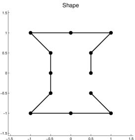
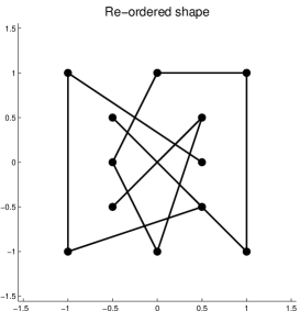
Figure 2: Two observations of the same shape, described by the positions of a set of landmarks, here represented by the black dots. The line connecting the dots, represented only for illustrative purposes, indicates the order by which the points are stored. Thus, although the left and right images represent the same shape, this is not trivially inferred from the stored data.

We compute the ANSIG of each of the shapes in Fig. 2. As expected, although the vectors containing the landmarks for these two shapes are completely different (due to re-ordering), we obtain the same ANSIG, which is represented in Fig. 3. This illustrates that the ANSIG is a permutation invariant representation. Obviously, the discrete counterparts of the ANSIGs, i.e., their samples on the unit-circle, also represented in Fig. 3, are also equal. Since the ANSIGs of geometrically different shapes result distinct, this signature is a substitute of the abstract quotient map $\pi$ in Fig. 1. The reader may also wonder why the middle and right plots in Fig. 3 are periodic (period $\pi$). This fact is due to the rotational symmetry (of $\pi$) of the shapes represented in Fig. 2. We postpone to the following section a more detailed comment on this aspect.

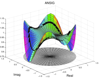
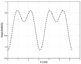
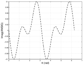
Figure 3: The ANSIG of the shapes in Fig. 2. In the left, the real part is represented by the surface high and the imaginary part by its color. In the middle and right plots, the discrete version of the ANSIG, i.e., its unit-circle samples. Although the vectors containing the shapes in Fig. 2 are distinct, due to re-ordering, their ANSIGs results equal, as desired.

III Quotienting out shape-preserving geometric transformations

We now address how the ANSIG representation handles shape-preserving geometric transformations, such as translation, rotation and scale. For reasons that will become clear below, we require that the shape vector ${\boldsymbol{z}}=[\,z_{1}\,z_{2}\,\cdots\,z_{n}\,]^{T}$ does not have all its entries with the same value, i.e., we require that ${\boldsymbol{z}}\in{\mathbb{C}}_{\ast}^{n}$, where ${\mathbb{C}}_{\ast}^{n}={\mathbb{C}}^{n}-\{[\,z\,z\,\cdots\,z\,]^{T}:\,z\in{\mathbb{C}}\}$ (note that only the pathological cases when all the landmarks collapse into a single point are excluded).

As introduced in the previous section, a shape is an orbit generated by a group $G$ of plausible transformations. Our main goal is to conceive a computationally efficient mechanism to detect if two given vectors ${\boldsymbol{z}},{\boldsymbol{w}}\in{\mathbb{C}}_{\ast}^{n}$ are in the same orbit, i.e., if they represent the same shape. In the previous section, we considered the permutation group $G=\Pi(n)$, i.e., we considered that ${\boldsymbol{z}}$ and ${\boldsymbol{w}}$ represent the same shape if they are equal up to a permutation. We introduced a maximal invariant with respect to this group: the ANSIG $a:\,{\mathbb{C}}_{\ast}^{n}\rightarrow{\mathcal{A}}$ is such that $a({\boldsymbol{z}},\cdot)=a({\boldsymbol{w}},\cdot)$ if and only if ${\boldsymbol{z}}$ and ${\boldsymbol{w}}$ are in the same orbit. Building on this result, we now extend the group $G$ to also accommodate shape-preserving geometric transformations.

III-A Group of geometric transformations

Naturally, two vectors ${\boldsymbol{z}},{\boldsymbol{w}}\in{\mathbb{C}}_{\ast}^{n}$ represent the same shape if they are equal, up to, not only a permutation of their entries, but also a translation, rotation, and scale factor, affecting the set of points they represent in the plane. To take this into account, we consider the group of transformations $G=\Pi(n)\times{\mathbb{C}}\times{\mathbb{S}}^{1}\times{\mathbb{R}}^{+}$, where $\Pi(n)$ is the set of permutation matrices, ${\mathbb{S}}^{1}$ is the unit-circle in the complex plane, and ${\mathbb{R}}^{+}$ is the set of positive real numbers. We then consider the action of $G$ on ${\mathbb{C}}_{\ast}^{n}$ as the map $G\times{\mathbb{C}}_{\ast}^{n}\rightarrow{\mathbb{C}}_{\ast}^{n}$, defined by

$$\left({\boldsymbol{\Pi}},t,e^{j\theta},\lambda\right)\cdot{\boldsymbol{z}}=\lambda e^{j\theta}{\boldsymbol{\Pi}}{\boldsymbol{z}}+t{\boldsymbol{1}}_{n}\,,$$ (16)

where ${\boldsymbol{1}}_{n}=[\,1\,1\,\cdots\,1\,]^{T}$ is the $n$-dimensional vector with all entries equal to $1$. It is clear from (16) that the action of an element of the group $G$ on a given vector ${\boldsymbol{z}}$ corresponds to a permutation (${\boldsymbol{\Pi}}$), translation ($t$), rotation ($\theta$), and scaling ($\lambda$), applied to the shape in ${\boldsymbol{z}}$. Naturally, the group operation takes into account the composition of rigid geometric transformations:

$$\left({\boldsymbol{\Pi}}_{1},t_{1},e^{j\theta_{1}},\lambda_{1}\right)\cdot\left({\boldsymbol{\Pi}}_{2},t_{2},e^{j\theta_{2}},\lambda_{2}\right)\cdot{\boldsymbol{z}} = \left({\boldsymbol{\Pi}}_{1},t_{1},e^{j\theta_{1}},\lambda_{1}\right)\cdot\left(\lambda_{2}e^{j\theta_{2}}{\boldsymbol{\Pi}}_{2}{\boldsymbol{z}}+t_{2}{\boldsymbol{1}}_{n}\right)$$ (17)

$$= \lambda_{1}e^{j\theta_{1}}{\boldsymbol{\Pi}}_{1}\left(\lambda_{2}e^{j\theta_{2}}{\boldsymbol{\Pi}}_{2}{\boldsymbol{z}}+t_{2}{\boldsymbol{1}}_{n}\right)+t_{1}{\boldsymbol{1}}_{n}$$

$$= \lambda_{1}\lambda_{2}e^{j(\theta_{1}+\theta_{2})}{\boldsymbol{\Pi}}_{1}{\boldsymbol{\Pi}}_{2}{\boldsymbol{z}}+\lambda_{1}e^{j\theta_{1}}t_{2}{\boldsymbol{1}}_{n}+t_{1}{\boldsymbol{1}}_{n}$$

$$= \left({\boldsymbol{\Pi}}_{1}{\boldsymbol{\Pi}}_{2},\lambda_{1}e^{j\theta_{1}}t_{2}+t_{1},e^{j(\theta_{1}+\theta_{2})},\lambda_{1}\lambda_{2}\right)\cdot{\boldsymbol{z}}\,.$$

The shapes that are equal to the instance ${\boldsymbol{z}}$, up to a permutation, translation, rotation, and scale, form the orbit $[{\boldsymbol{z}}]$, the set obtained by considering the action of all elements of $G$ on ${\boldsymbol{z}}$,

$$[{\boldsymbol{z}}]=\left\{\left({\boldsymbol{\Pi}},t,e^{j\theta},\lambda\right)\cdot{\boldsymbol{z}}:\,\left({\boldsymbol{\Pi}},t,e^{j\theta},\lambda\right)\in G\right\}.$$ (18)

The problem of deciding if two given vectors ${\boldsymbol{z}}$, ${\boldsymbol{w}}$ represent the same shape, i.e., if they are in the same orbit, corresponds to checking if the value of the optimization problem

$$\min_{\left({\boldsymbol{\Pi}},t,e^{j\theta},\lambda\right)\in G}\;\left\|{\boldsymbol{z}}-\left({\boldsymbol{\Pi}},t,e^{j\theta},\lambda\right)\cdot{\boldsymbol{w}}\right\|$$ (19)

is zero (or, in practice, below a small threshold, due to the noise). To the best of our knowledge, solving (19) without making use of permutation invariant representations requires an exhaustive search over the set $\Pi(n)$, which has cardinality $n!$. Clearly, this is not feasible, even for moderate values of the number of landmarks, say $n=100$ ($100!\simeq 10^{158}$). In opposition, in our experiments, we use shapes described by very large sets of points, e.g., with $n$ up to $40000$.

III-B Translation and scale

We use the ANSIG map to devise a scheme that circumvents the combinatorial search in (19). We start by quotienting out all the transformations, except the rotation, through a map $\phi:\,{\mathbb{C}}_{\ast}^{n}\rightarrow{\mathcal{A}}$. Then, we show that $\phi$ is equivariant with respect to the rotations, i.e., that its action commutes with the one of the group of rotations. This will enable a computationally simple scheme to decide from $\phi({\boldsymbol{z}})$ and $\phi({\boldsymbol{w}})$ if the vectors ${\boldsymbol{z}}$ and ${\boldsymbol{w}}$ correspond to the same shape.

To factor out translation and scale, we pre-process the shape vector, through centering and normalization, before computing its signature. This corresponds to considering the composite map $\phi:\,{\mathbb{C}}_{\ast}^{n}\rightarrow{\mathcal{A}}$, defined by

$$\phi({\boldsymbol{z}},\cdot)=a\left(\sqrt{n}\frac{\mbox{${\boldsymbol{z}}-\overline{\boldsymbol{z}}$}}{\mbox{$\left\|{\boldsymbol{z}}-\overline{\boldsymbol{z}}\right\|$}},\cdot\right)\,,$$ (20)

where $a$ is given by (8), $\overline{\boldsymbol{z}}$ is a vector with all entries equal to the mean value of $\boldsymbol{z}$, i.e., $\overline{\boldsymbol{z}}=\frac{1}{n}{\boldsymbol{1}}_{n}^{T}{\boldsymbol{z}}{\boldsymbol{1}}_{n}$ , and $\left\|\cdot\right\|$ denotes the 2-norm, i.e., $\left\|{\boldsymbol{z}}\right\|=\sqrt{{\boldsymbol{z}}^{T}{\boldsymbol{z}}}$. It becomes clear now why we excluded the shape vectors with all equal entries, i.e., why we imposed ${\boldsymbol{z}}\in{\mathbb{C}}_{\ast}^{n}$: this guarantees ${\boldsymbol{z}}\neq\overline{\boldsymbol{z}}$, thus $\left\|{\boldsymbol{z}}-\overline{\boldsymbol{z}}\right\|\neq 0$ in (20). Since in the remaining of the paper we focus in comparing shapes affected by the above mentioned geometric transformations, we make $\phi$ supersede $a$, i.e., we refer to the analytic function $\phi({\boldsymbol{z}},\cdot)$ as the analytic signature (ANSIG) of the shape ${\boldsymbol{z}}$, and to the composite map $\phi$ in (20) as the ANSIG map.

The reader may wonder why the factor $\sqrt{n}$ in (20). In fact, this factor has nothing to do with factoring out translation or scale — it is constant for shapes described by the same number $n$ of landmarks. The motivation for this factor is precisely to enable dealing with shapes described by different numbers of landmarks, providing robustness to over/under sampling the shapes. To demonstrate this capability, consider an extreme example, where each landmark in the $n$-dimensional vector ${\boldsymbol{z}}\in{\mathbb{C}}_{\ast}^{n}$ is repeated $p$ times, leading to the $pn$-dimensional vector ${\boldsymbol{z}}_{p}$, i.e.,

$${\boldsymbol{z}}_{p}={\boldsymbol{1}}_{p}\otimes{\boldsymbol{z}}\,,$$ (21)

where $\otimes$ is the Kronecker product. Naturally, ${\boldsymbol{z}}$ and ${\boldsymbol{z}}_{p}$ represent the same shape. We now show that the factor $\sqrt{n}$ in (20) guarantees that they have the same ANSIG.

To simplify the notation, name ${\boldsymbol{w}}$ the post-processed version of the shape vector ${\boldsymbol{z}}$, i.e.,

$${\boldsymbol{w}}=\sqrt{n}\frac{\mbox{${\boldsymbol{z}}-\overline{\boldsymbol{z}}$}}{\mbox{$\left\|{\boldsymbol{z}}-\overline{\boldsymbol{z}}\right\|$}}\,.$$ (22)

From the relation between ${\boldsymbol{z}}_{p}$ and ${\boldsymbol{z}}$ in (21), it immediately follows that

$${\boldsymbol{z}}_{p}-\overline{\boldsymbol{z}}_{p}={\boldsymbol{1}}_{p}\otimes\left({\boldsymbol{z}}-\overline{\boldsymbol{z}}\right)\qquad\mbox{and}\qquad\left\|{\boldsymbol{z}}_{p}-\overline{\boldsymbol{z}}_{p}\right\|=\sqrt{p}\left\|{\boldsymbol{z}}-\overline{\boldsymbol{z}}\right\|\,,$$ (23)

thus the post-processed version of ${\boldsymbol{z}}_{p}$ is just the $p$-times replication of the one of ${\boldsymbol{z}}$ in (22),

$$\sqrt{pn}\frac{\mbox{${\boldsymbol{z}}_{p}-\overline{\boldsymbol{z}}_{p}$}}{\mbox{$\left\|{\boldsymbol{z}}_{p}-\overline{\boldsymbol{z}}_{p}\right\|$}}=\sqrt{n}\frac{\mbox{${\boldsymbol{1}}_{p}\otimes({\boldsymbol{z}}-\overline{\boldsymbol{z}})$}}{\mbox{$\left\|{\boldsymbol{z}}-\overline{\boldsymbol{z}}\right\|$}}={\boldsymbol{1}}_{p}\otimes{\boldsymbol{w}}\,.$$ (24)

The ANSIG of ${\boldsymbol{z}}_{p}$ is now successively written as

$$\phi({\boldsymbol{z}}_{p},\xi) = a\left({\boldsymbol{1}}_{p}\otimes{\boldsymbol{w}},\xi\right)$$ (25)

$$= \frac{1}{pn}\left(\rule{0.0pt}{12.91663pt}\right.\underbrace{\sum_{m=1}^{n}e^{w_{m}\xi}+\sum_{m=1}^{n}e^{w_{m}\xi}+\cdots+\sum_{m=1}^{n}e^{w_{m}\xi}}_{\mbox{$p$ times}}\left.\rule{0.0pt}{12.91663pt}\right)$$ (26)

$$= \frac{1}{n}\sum_{m=1}^{n}e^{w_{m}\xi}$$ (27)

$$= a({\boldsymbol{w}},\xi)$$ (28)

$$= \phi({\boldsymbol{z}},\xi)\,,$$ (29)

establishing the desired equality between the signatures of ${\boldsymbol{z}}_{p}$ and ${\boldsymbol{z}}$. Equalities (25) and (29) come from the definition of $\phi$ in (20); in (26) and (28) we used the definition of $a$ in (8).

Maximal invariance with respect to permutation, translation, and scale. We now show that $\phi$ is a maximal invariant with respect to all transformations, except rotation, i.e., that two shapes have the same ANSIG if and only if they are equal up to permutation, translation, and scale.

The maximal invariance of $\phi$ can be formalized as

$$\phi({\boldsymbol{z}},\cdot)=\phi({\boldsymbol{w}},\cdot)\;\Leftrightarrow\;{\boldsymbol{z}}=\left({\boldsymbol{\Pi}},t,1,\lambda\right)\cdot{\boldsymbol{w}}\,,$$ (30)

for some $({\boldsymbol{\Pi}},t,1,\lambda)\in G$. The invariance, i.e., the sufficiency part ($\Leftarrow$) of (30), is straightforward:

$$\phi({\boldsymbol{z}},\cdot) = \phi\left(\left({\boldsymbol{\Pi}},t,1,\lambda\right)\cdot{\boldsymbol{w}},\cdot\right)$$ (31)

$$= \phi\left(\lambda{\boldsymbol{\Pi}}{\boldsymbol{w}}+t{\boldsymbol{1}}_{n},\cdot\right)$$ (32)

$$= a\left(\sqrt{n}\frac{\lambda{\boldsymbol{\Pi}}{\boldsymbol{w}}+t{\boldsymbol{1}}_{n}-\overline{\lambda{\boldsymbol{\Pi}}{\boldsymbol{w}}+t{\boldsymbol{1}}_{n}}}{\left\|\lambda{\boldsymbol{\Pi}}{\boldsymbol{w}}+t{\boldsymbol{1}}_{n}-\overline{\lambda{\boldsymbol{\Pi}}{\boldsymbol{w}}+t{\boldsymbol{1}}_{n}}\right\|},\cdot\right)$$ (33)

$$= a\left(\sqrt{n}\frac{{\boldsymbol{\Pi}}\left({\boldsymbol{w}}-\overline{{\boldsymbol{w}}}\right)}{\left\|{\boldsymbol{w}}-\overline{{\boldsymbol{w}}}\right\|},\cdot\right)$$ (34)

$$= a\left(\sqrt{n}\frac{{\boldsymbol{w}}-\overline{{\boldsymbol{w}}}}{\left\|{\boldsymbol{w}}-\overline{{\boldsymbol{w}}}\right\|},\cdot\right)$$ (35)

$$= \phi({\boldsymbol{w}},\cdot)\,,$$ (36)

where we just used the definition of $\phi$, standard manipulation of matrices and vectors in (34), and the invariance of $a$ with respect to permutations in (35).

We now prove the maximal invariance, i.e., the necessity part ($\Rightarrow$) of the equivalence (30). Naturally, the maximal invariance of $\phi$ also hinges on the maximal invariance of $a$ established in the previous section. Suppose that $\phi({\boldsymbol{z}},\cdot)=\phi({\boldsymbol{w}},\cdot)$. Then, from the definition of $\phi$ in (20),

$$a\left(\sqrt{n}\frac{\mbox{${\boldsymbol{z}}-\overline{\boldsymbol{z}}$}}{\mbox{$\left\|{\boldsymbol{z}}-\overline{\boldsymbol{z}}\right\|$}},\cdot\right)=a\left(\sqrt{n}\frac{\mbox{${\boldsymbol{w}}-\overline{\boldsymbol{w}}$}}{\mbox{$\left\|{\boldsymbol{w}}-\overline{\boldsymbol{w}}\right\|$}},\cdot\right)\,,$$ (37)

and, by the maximal invariance of $a$ with respect to permutations, equality (37) implies that

$$\sqrt{n}\frac{\mbox{${\boldsymbol{z}}-\overline{\boldsymbol{z}}$}}{\mbox{$\left\|{\boldsymbol{z}}-\overline{\boldsymbol{z}}\right\|$}}={\boldsymbol{\Pi}}\sqrt{n}\frac{\mbox{${\boldsymbol{w}}-\overline{\boldsymbol{w}}$}}{\mbox{$\left\|{\boldsymbol{w}}-\overline{\boldsymbol{w}}\right\|$}}\,,$$ (38)

for some ${\boldsymbol{\Pi}}\in\Pi(n)$. The relation between ${\boldsymbol{z}}$ and ${\boldsymbol{w}}$ in (38) can be rewritten as

$${\boldsymbol{z}}=\frac{\left\|{\boldsymbol{z}}-\overline{\boldsymbol{z}}\right\|}{\left\|{\boldsymbol{w}}-\overline{\boldsymbol{w}}\right\|}{\boldsymbol{\Pi}}{\boldsymbol{w}}-\frac{\left\|{\boldsymbol{z}}-\overline{\boldsymbol{z}}\right\|}{\left\|{\boldsymbol{w}}-\overline{\boldsymbol{w}}\right\|}\overline{\boldsymbol{w}}+\overline{\boldsymbol{z}}\,.$$ (39)

It is now clear that this relation is of the form ${\boldsymbol{z}}=\lambda{\boldsymbol{\Pi}}{\boldsymbol{w}}+t{\boldsymbol{1}}_{n}$, establishing that ${\boldsymbol{z}}=({\boldsymbol{\Pi}},t,1,\lambda)\cdot{\boldsymbol{w}}$ for a particular choice of $({\boldsymbol{\Pi}},t,1,\lambda)\in G$, thus completing the proof of (30); just define

$$\lambda=\frac{\mbox{$\left\|{\boldsymbol{z}}-\overline{\boldsymbol{z}}\right\|$}}{\mbox{$\left\|{\boldsymbol{w}}-\overline{\boldsymbol{w}}\right\|$}}>0\qquad\mbox{ and }\quad t=\frac{1}{n}{\boldsymbol{1}}_{n}^{T}\left({\boldsymbol{z}}-\lambda{\boldsymbol{w}}\right)\,\in{\mathbb{C}}\,.$$ (40)

III-C Rotation

We have seen that the ANSIG map $\phi$ quotients out all transformations in $G$, except the rotation. We now show that although $\phi$ is not invariant to rotations, it is equivariant, i.e., that its action commutes with the one of the group of rotations. Naturally, this equivariance is inherited from the map $a$ in (8). Let us then start by looking at how the rotation of a shape ${\boldsymbol{z}}$ affects the analytic function produced by the map $a$. The rotated version of the shape is simply $e^{j\theta}{\boldsymbol{z}}$. From the definition of $a$ in (8), it follows that

$$a(e^{j\theta}{\boldsymbol{z}},\xi)=\frac{1}{n}\sum_{k=1}^{n}e^{e^{j\theta}z_{k}\xi}=\frac{1}{n}\sum_{k=1}^{n}e^{z_{k}\left(e^{j\theta}\xi\right)}=a({\boldsymbol{z}},e^{j\theta}\xi)\,.$$ (41)

Equivariance with respect to rotation. The property just derived (41) leads immediately to the equivariance of the ANSIG map $\phi$, through the following sequence of equalities:

$$\phi\left(({\boldsymbol{\Pi}},t,e^{j\theta},\lambda)\cdot{\boldsymbol{z}},\xi\right) = \phi\left(\lambda e^{j\theta}{\boldsymbol{\Pi}}{\boldsymbol{z}}+t{\boldsymbol{1}}_{n},\xi\right)$$ (42)

$$= a\left(\sqrt{n}\frac{e^{j\theta}{\boldsymbol{\Pi}}\left({\boldsymbol{z}}-\overline{\boldsymbol{z}}\right)}{\left\|{\boldsymbol{z}}-\overline{\boldsymbol{z}}\right\|},\xi\right)$$ (43)

$$= a\left(\sqrt{n}\frac{\mbox{$e^{j\theta}({\boldsymbol{z}}-\overline{\boldsymbol{z}})$}}{\mbox{$\left\|{\boldsymbol{z}}-\overline{\boldsymbol{z}}\right\|$}},\xi\right)$$ (44)

$$= a\left(\sqrt{n}\frac{\mbox{${\boldsymbol{z}}-\overline{\boldsymbol{z}}$}}{\mbox{$\left\|{\boldsymbol{z}}-\overline{\boldsymbol{z}}\right\|$}},e^{j\theta}\xi\right)$$ (45)

$$= \phi({\boldsymbol{z}},e^{j\theta}\xi)\,,$$ (46)

where (43) and (46) use the definition of $\phi$ in (20) and simple manipulations, (44) uses the invariance of $a$ with respect to permutations, and (45) comes from (41).

We thus conclude that the rotation of a shape propagates to its signature, i.e., the ANSIG of the rotated shape is simply a rotated version (in the complex plane) of the ANSIG of the original shape. Obviously, the equivariance is inherited by the restriction of the ANSIG to the unit-circle, $\phi_{{\mathbb{S}}^{1}}:\,{\mathbb{C}}_{\ast}^{n}\times{\mathbb{S}}^{1}\rightarrow{\mathbb{C}}$, $\phi_{{\mathbb{S}}^{1}}({\boldsymbol{z}},\xi)=\phi({\boldsymbol{z}},\xi)$:

$$\phi_{{\mathbb{S}}^{1}}\left(\left({\boldsymbol{\Pi}},t,e^{j\theta},\lambda\right)\cdot{\boldsymbol{z}},\xi\right)=\phi_{{\mathbb{S}}^{1}}\left({\boldsymbol{z}},e^{j\theta}\xi\right)\,.$$ (47)

Equality of orbits. In summary, two vectors are in the same orbit of the group G of relevant transformations, i.e., they represent the same shape, up to permutation, translation, rotation, and scale, iif (the restriction to the unit-circle of) their ANSIGs are equal, up to a rotation:

$$\mbox{${\boldsymbol{z}}$ and ${\boldsymbol{w}}$ represent the same shape}\;\Leftrightarrow\;\phi_{{\mathbb{S}}^{1}}({\boldsymbol{z}},\cdot)=\phi_{{\mathbb{S}}^{1}}\left({\boldsymbol{w}},e^{j\theta}\,\cdot\right),\,\mbox{for some }\theta\in[0,2\pi].$$ (48)

The necessity part of this claim ($\Rightarrow$) comes immediately from (47). To prove the sufficiency ($\Leftarrow$), suppose that $\phi_{{\mathbb{S}}^{1}}({\boldsymbol{z}},\cdot)=\phi_{{\mathbb{S}}^{1}}\left({\boldsymbol{w}},e^{j\theta}\,\cdot\right)$, for some $\theta\in[0,2\pi]$. This means that

$$\phi({\boldsymbol{z}},e^{j\varphi})=\phi({\boldsymbol{w}},e^{j\theta}e^{j\varphi})\,,\quad\mbox{ for all }\varphi\in[0,2\pi].$$ (49)

Using the equivariance of $\phi$, derived in (42-46), in the right-hand side of (49), we get

$$\phi({\boldsymbol{z}},e^{j\varphi})=\phi(e^{j\theta}{\boldsymbol{w}},e^{j\varphi})\,,\quad\mbox{ for all }\varphi\in[0,2\pi]\,,$$ (50)

stating that the analytic functions $\phi({\boldsymbol{z}},\cdot)$ and $\phi(e^{j\theta}{\boldsymbol{w}},\cdot)$ coincide on the unit-circle, thus, on the entire complex plane:

$$\phi({\boldsymbol{z}},\cdot)=\phi(e^{j\theta}{\boldsymbol{w}},\cdot)\,.$$ (51)

From the maximal invariance of the map $\phi$, stated in (30), equality (51) is equivalent to

$${\boldsymbol{z}}=({\boldsymbol{\Pi}},t,1,\lambda)\cdot e^{j\theta}{\boldsymbol{w}}\,,$$ (52)

for some $({\boldsymbol{\Pi}},t,1,\lambda)\in G$. Using the composition of elements of G, expressed in (17), equality (52) can be rewritten as ${\boldsymbol{z}}=({\boldsymbol{\Pi}},t,e^{j\theta},\lambda)\cdot{\boldsymbol{w}}$, which shows that ${\boldsymbol{z}}$ and ${\boldsymbol{w}}$ are in the same orbit, i.e., that they represent the same shape.

III-D Illustrations

We now illustrate the behavior of the ANSIG representation in what respects to the properties studied in this section, i.e., dealing with shape-preserving geometric transformations and with shapes described by point sets of different cardinality (i.e., with different sampling density).

Shape-preserving transformations. We use the binary images shown in Fig. 4 which, besides a point permutation (not seen in the images), also differ by translation, rotation, and scale factors (easily perceived due to different position, orientation, and scale of the shapes).

         

Figure 4: Two shapes that differ by a geometric transformation: the right one is obtained by translating, rotating, and resizing the left one. The ordering of the points describing the shapes is also made distinct on purpose, as in the example of Fig. 2.

We computed the (unit-circle samples of the) ANSIGs of the shapes in Fig. 4, obtaining the magnitude and phase plots in Fig. 5. Note that, in spite of the different vectors describing the shapes in Fig. 4, both ANSIG plots in Fig. 5 only differ by a (circular) translation. This is in agreement with what we concluded in this section, see expression (47): permutation, translation, and scale, are factored out; the rotation of a shape induces the same rotation on its ANSIG, thus a (circular) translation of the magnitude and phase plots of its restriction to the unit-circle. The rotation that aligns the shapes can be efficiently computed, as will be described in Section IV.

         

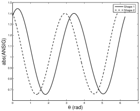
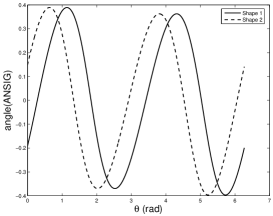
Figure 5: Magnitude and phase of the ANSIGs of the two shapes of Fig. 4. Note that, although these shapes differ by position, rotation, scale, and point labeling, their ANSIGs only differ by a (circular) translation that can be easily computed.

Different sampling density. The experiment above used shapes described by sets of points of the same cardinality. We now illustrate that the ANSIG also copes with shapes described by point sets of (very) different cardinality, as also discussed in this section. This characteristic is very important in practice, e.g., to deal with shapes obtained from images of different resolutions (due do the pixelization, the same shape usually leads to point sets of different cardinality).

We use the shapes represented in Fig. 6. Both represent the same object but the shape in the right is described by just $30\%$ of the points of the one in the left. In Fig. 7, we represent the ANSIGs of both shapes. As easily seen, the ANSIGs of the differently sampled shapes almost coincide, as desired, and anticipated in this section, see the insight provided by expressions (25-29). All our tests confirmed that the ANSIG representation deals well with different sampling densities, at leat as far as the corresponding shapes are recognizable by an human.

         

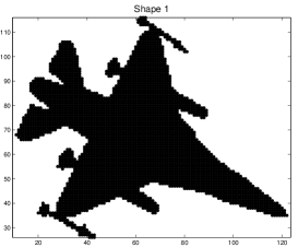
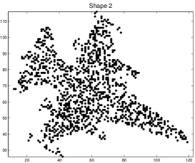
Figure 6: Similar shapes with different sampling density. The right image has 30% of the points of the left one.

         

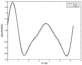
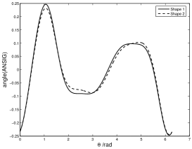
Figure 7: Magnitude and phase of the ANSIGs of the shapes in Fig. 6. Although the number of points describing these shapes differ significantly, their ANSIGs result similar, as desired.

We finally comment on the fact that the ANSIG plots in Fig. 3 of the previous section are periodic (they exhibit not only the $2\pi$ periodicity of any ANSIG but also a smaller fundamental period of $\pi$). This periodicity is due the fact that the shape corresponding to those plots is invariant under rotations of multiples of $\pi$ (see Fig. 2). Since shape rotation leads to a translation of the ANSIG plots, the plots for the shape in Fig. 2 result invariant to translations of multiples of $\pi$, i.e., they are periodic with period $\pi$, therefore two periods appear in the interval $[0,2\pi]$. Naturally, this does not happen with shapes that do not exhibit rotational symmetry, e.g., the ones in Figs. 4 and 6, whose ANSIG plots in Figs. 5 and  7 exhibit only $2\pi$ periodicity.

IV Shape-based recognition

In this section we describe how the ANSIG representation can be used for rigid shape recognition. Since our representation is invariant to (or deals gracefully with) the relevant transformations (point labeling, translation, rotation, and scale), we are able to perform shape classification using a very simple scheme: the shape database is just composed by the ANSIGs of prototype shapes (a single prototype per shape class); classification boils down to comparing the ANSIG of a candidate shape with the ones in the database.

Our experiments show that the invariance of the ANSIG representation enables dealing with noise and distortions typical of shapes obtained from real images, with the simple strategy just outlined, avoiding this way computationally complex learning schemes. We emphasize, however, that the ANSIG representation can be incorporated in more sophisticated classification procedures if non-rigid shape classification is the goal. For example, storing the ANSIGs of several prototypes per class and using k-NN (nearest neighbors) classification is straightforward.

IV-A Efficient comparison of ANSIGs

As described in Section II, a practical way to implement the map $a:\,{\mathbb{C}}_{\ast}^{n}\rightarrow{\mathcal{A}}$ is through its unit-circle sampled version $a_{K}:\,{\mathbb{C}}^{n}_{\ast}\rightarrow{\mathbb{C}}^{K}$, introduced in (15). Thus, in practice, the unit-circle ANSIG restriction $\phi_{{\mathbb{S}}^{1}}$ is approximated by its sampled version $\phi_{K}:\,{\mathbb{C}}_{\ast}^{n}\rightarrow{\mathbb{C}}^{K}$, given by

$$\phi_{K}({\boldsymbol{z}})=a_{K}\left(\sqrt{n}\frac{\mbox{${\boldsymbol{z}}-\overline{\boldsymbol{z}}$}}{\mbox{$\left\|{\boldsymbol{z}}-\overline{\boldsymbol{z}}\right\|$}}\right)\,,$$ (53)

where, we recall, $K$ denotes the number of samples on the unit-circle. Naturally, with $K$ sufficiently large, any rotation $e^{j\theta}$ is well approximated by a point in the unit-circle sampling grid, i.e., $e^{j\theta}\simeq e^{j\frac{2\pi}{K}k}=W_{K}^{k}$, thus the equivariance of $\phi_{{\mathbb{S}}^{1}}$, expressed in (47), gracefully transfers to its discrete version $\phi_{K}$, as

$$\phi_{K}\left(\left({\boldsymbol{\Pi}},\lambda,v,e^{i\theta}\right)\cdot{\boldsymbol{z}}\right)\simeq\phi_{K}({\boldsymbol{z}})\,{\sf mod}\,k\,,$$ (54)

where ${\sf mod}\,k$ denotes a $k$-step cyclic shift.

Our test for deciding if two point vectors ${\boldsymbol{z}}$ and ${\boldsymbol{w}}$ correspond to the same shape, i.e., for the equality of the orbits of ${\boldsymbol{z}}$ and ${\boldsymbol{w}}$, expressed in (48), leads to checking if $\phi_{K}({\boldsymbol{w}})$ is a cyclic-shifted version of $\phi_{K}({\boldsymbol{z}})$, i.e., if

$$\phi_{K}({\boldsymbol{z}})\simeq\phi_{K}({\boldsymbol{w}})\,{\sf mod}\,k\,,\qquad\mbox{ for some }\;k=0,1,\ldots,K-1.$$ (55)

This test can be carried out by computing the cyclic-shift $k^{*}$ that best “aligns” the vectors,

$$k^{*}=\arg\min_{k=0,1,\ldots,K-1}\left\|\phi_{K}({\boldsymbol{z}})-\phi_{K}({\boldsymbol{w}})\,{\sf mod}\,k\right\|^{2}\,,$$ (56)

and then checking the similarity of the corresponding “aligned” versions.

Solving (56) by computing $\phi_{K}({\boldsymbol{w}})\,{\sf mod}\,k$ and comparing it with $\phi_{K}({\boldsymbol{z}})$, for each $k$, leads to an algorithm with computational complexity ${\mathcal{O}}(K^{2})$. We now present a computationally simpler scheme, based on the Fast Fourier Transform (FFT). We denote the Discrete Fourier Transform (DFT) of a vector ${\boldsymbol{v}}\in{\mathbb{C}}^{K}$ by the vector $\widehat{\boldsymbol{v}}\in{\mathbb{C}}^{K}$, given by

$$\widehat{\boldsymbol{v}}={\boldsymbol{D}}_{K}^{H}{\boldsymbol{v}}\,,\qquad\mbox{with}\qquad{\boldsymbol{d}}_{k}=\frac{1}{\sqrt{K}}\begin{bmatrix}1&W_{K}^{k}&W_{K}^{2k}&W_{K}^{3k}&\cdots&W_{K}^{(K-1)k}\end{bmatrix}^{T}\,.$$ (57)

In (57), ${\boldsymbol{D}}_{K}$ is the $K\times K$ DFT matrix [40], ${\boldsymbol{D}}_{K}^{H}$ denotes its conjugate transpose (also known as the Hermitian), and ${\boldsymbol{d}}_{k}$ is the $k^{\mbox{\small th}}$ column of ${\boldsymbol{D}}_{K}$.

Using Parseval’s relation [40], which is based on the fact that the DFT is an unitary operator (${\boldsymbol{D}}_{K}^{H}{\boldsymbol{D}}_{K}={\boldsymbol{I}}_{K})$, the minimization (56) is written in the frequency domain as

$$k^{*}=\arg\min_{k=0,1,\ldots,K-1}\left\|\widehat{\phi_{K}({\boldsymbol{z}})}-\widehat{\phi_{K}({\boldsymbol{w}})\,{\sf mod}\,k}\right\|^{2}\,.$$ (58)

Since the DFT of a $k$-cyclic-shifted version of a signal equals the DFT of the original signal multiplied by the exponential sequence $\sqrt{K}{\boldsymbol{d}}_{k}$ [40], expression (58) is equivalent to

$$k^{*}=\arg\min_{k=0,1,\ldots,K-1}\left\|\widehat{\phi_{K}({\boldsymbol{z}})}-\widehat{\phi_{K}({\boldsymbol{w}})}\odot\sqrt{K}\,{\boldsymbol{d}}_{k}\right\|^{2}\,,$$ (59)

where $\odot$ denotes the elementwise (also known as Schur or Hadammard) product. Removing from the norm in (59) the terms that do not depend on $k$, we finally get

$$k^{*}=\arg\max_{k=0,1,\ldots,K-1}{\sf Re}\left\{{\boldsymbol{d}}_{k}^{H}\left[{\widehat{\phi_{K}({\boldsymbol{z}})}}\odot\overline{\widehat{\phi_{K}({\boldsymbol{w}})}}\right]\right\}\,,$$ (60)

where $\overline{{\boldsymbol{v}}}$ denotes the conjugate of ${\boldsymbol{v}}$ and ${\sf Re}\left\{{\boldsymbol{v}}\right\}$ its real part.

Expression (60) provides a computational simple scheme to compute the shift $k^{*}$ that best “aligns” the ANSIGs $\phi_{K}({\boldsymbol{z}})$ and $\phi_{K}({\boldsymbol{w}})$ of two shape vectors ${\boldsymbol{z}}$ and ${\boldsymbol{w}}$: i) compute the DFTs $\widehat{\phi_{K}({\boldsymbol{z}})}$ and $\widehat{\phi_{K}({\boldsymbol{w}})}$; ii) compute the elementwise product $\widehat{\phi_{K}({\boldsymbol{z}})}\odot\overline{\widehat{\phi_{K}({\boldsymbol{w}})}}$; iii) compute the DFT of this product and locate the entry with largest real part. Since each DFT is computed by using the FFT algorithm, which has computational complexity ${\mathcal{O}}(K\log K)$, the overall complexity of our comparison scheme is ${\mathcal{O}}(K+3K\log K)$.

Finally, to measure the similarity between the shapes in ${\boldsymbol{z}}$ and ${\boldsymbol{w}}$, i.e., the similarity between their “aligned” ANSIGs $\phi_{K}({\boldsymbol{z}})$ and $\phi_{K}({\boldsymbol{w}})\,{\mbox{{\sf mod}}}\,k^{*}$, we use the (cosine of the) angle between the corresponding vectors:

$$\psi(\mbox{\boldmath{$z$}},\mbox{\boldmath{$w$}})=\frac{\left|{\phi_{K}({\boldsymbol{z}})}^{T}\phi_{K}({\boldsymbol{w}})\,{\mbox{{\sf mod}}}\,k^{*}\right|}{\left\|{\phi_{K}({\boldsymbol{z}})}\right\|\,\left\|\phi_{K}({\boldsymbol{w}})\right\|}\,.$$ (61)

Thus, the similarity $\psi(\mbox{\boldmath{$z$}},\mbox{\boldmath{$w$}})$ is such that $0\leq\psi(\mbox{\boldmath{$z$}},\mbox{\boldmath{$w$}})\leq 1$ and the larger is $\psi(\mbox{\boldmath{$z$}},\mbox{\boldmath{$w$}})$, the more similar are the shapes in ${\boldsymbol{z}}$ and ${\boldsymbol{w}}$.

IV-B Improving robustness when dealing with interior shape detail

Before presenting experiments with shape classification, we anticipate that when a single ANSIG is used to describe a shape characterized by having specific details occurring at very different distances from the geometric center, the representation may lack the desired robustness. This is illustrated by the example in Figs. 8 and 9. Fig. 8 shows two shapes characterized by a similar large outer hexagon and distinct small inner polygons. The ANSIGs of these two shapes are represented in Fig. 9. As easily perceived, these signatures result very similar. Although one could argue that the shapes in Fig. 8 are in fact similar, the argument would be misleading, since if the small polygons were not in the center but in the periphery of the image, the ANSIGs would be far more distinct. We now briefly discuss this issue and ways to deal with it.

         

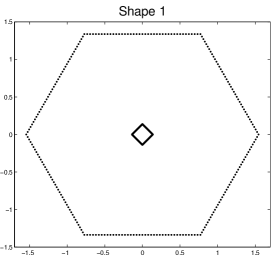
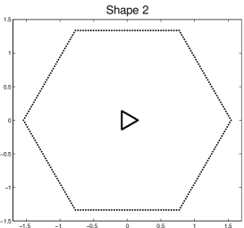
Figure 8: Two shapes that only differ in the points that are close to their center.

         

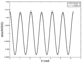
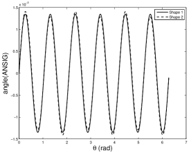
Figure 9: ANSIGs of the two shapes in Fig. 8. The similarity of the exterior hexagons makes the signatures very similar.

Weighted ANSIG. The similarity of the ANSIGs in Fig. 9 is explained by the exponential weighting of each landmark modulus (i.e., distance to the geometric center), when computing the map $a$ in (8), in which the ANSIG is based. In fact, representing the elements of a shape vector ${\boldsymbol{z}}$ by their polar coordinates, i.e., $z_{m}=\rho_{m}e^{j\theta_{m}}$, the map $a$ in (8) is written as

$$a({\boldsymbol{z}},\xi)=\frac{1}{n}\sum_{m=1}^{n}e^{\rho_{m}e^{j\theta_{m}}\xi}=\frac{1}{n}\sum_{m=1}^{n}e^{\rho_{m}}e^{e^{j\theta_{m}}\xi}\,,$$ (62)

which shows that landmarks at large distances from the origin (i.e., with large $\rho_{m}$), are taken into much larger account (exponential weighting) than those closer to the center (small $\rho_{m}$).

One approach to tackle this problem is precisely to weight the landmarks in a different way, with the care of maintaining the maximal invariance property. For example, if the shapes are preprocessed by an elementwise map $g$, that maps each entry $\rho_{m}e^{j\theta_{m}}$ to $\log\left(1+\rho_{m}\right)e^{j\theta_{m}}$, the signature obtained corresponds to replacing the map $a$ in (62) by a map $a_{g}$, given by:

$$a_{g}\left({\boldsymbol{z}},\xi\right)=a(g({\boldsymbol{z}}),\xi)=\frac{1}{n}\sum_{m=1}^{n}(1+\rho_{m})^{e^{j\theta_{m}}\xi}\,,$$ (63)

which now takes into account the modulus of the landmarks, i.e., their distance to the origin, in a linear way. It is straightforward to show that the maximal invariance of the ANSIG is not affected, because $g$ is an injection, i.e., there is a one-to-one mapping between ${\boldsymbol{z}}$ and $g({\boldsymbol{z}})$.

In Fig. 10 we shown the ANSIGs obtained for the shapes of Fig. 8, now using the differently weighted map $a_{g}$ in (63). Comparing the plots of Figs. 9 and 10, we see that the shape signatures are in fact more dissimilar, as desired, when the weighted version of the ANSIG is used.

         

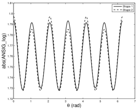
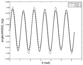
Figure 10: Magnitude and phase of the ANSIGs of the two shapes in Fig. 8, when the map $a$ in (8) is replaced by the weighted version $a_{g}$ in (63). As desired, the signatures result more distinct than the ones in Fig. 9.

Using more than one ANSIG. Rather than trying to describe shapes such as the ones in Fig. 8 with a single signature, an approach that must be considered is to use multiple descriptions. In fact, if we compute the ANSIGs of just the inner parts of these shapes, i.e., of the smaller inner polygons (the square and the triangle), we obtain the plots in Fig. 11, which are very distinct. This motivates the use of more than one ANSIG to distinguish between shapes like the ones in Fig. 8, i.e., shapes with similar outer content.

         

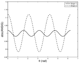
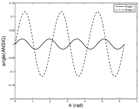
Figure 11: ANSIGs of the small square and triangle in the shapes of Fig. 8. Naturally, when this inner part is taken into account separately, the signatures result very distinct.

Although several hypothesis could be considered, we describe a simple way to implement a shape representation scheme based on two ANSIGs: the ANSIG of the entire set of landmarks, $\phi\left({\boldsymbol{z}}\right)$, and the ANSIG of some subset of inner landmarks, $\phi\left(\mbox{\boldmath{$z$}}_{{in}}\right)$. Naturally, $\mbox{\boldmath{$z$}}_{{in}}$ can be obtained from $z$ in several ways, e.g., by selecting the subset of points that have normalized absolute value smaller than one. Note that this joint signature keeps the invariance properties of the single ANSIG representation: the maximal invariance is obvious, since we maintain the ANSIG of the complete shape; the rotational equivariance comes from the fact that the partition is circular.

When comparing shapes ${\boldsymbol{z}}$ and ${\boldsymbol{w}}$ under this framework, the cyclic-shift $k^{*}$ that best “aligns” simultaneously both pairs of ANSIG vectors, $\phi_{K}\left(\mbox{\boldmath{$z$}}\right)$ with $\phi_{K}\left(\mbox{\boldmath{$w$}}\right)$ and $\phi_{K}\left(\mbox{\boldmath{$z$}}_{{in}}\right)$ with $\phi_{K}\left(\mbox{\boldmath{$w$}}_{{in}}\right)$ is obtained, by following steps similar to the ones in (56) to (60), as:

$$k^{*} = \arg\min_{k}\left\|\phi_{K}({\boldsymbol{z}})-\phi_{K}({\boldsymbol{w}})\,\mbox{{\sf mod}}\,k\right\|^{2}+\left\|\phi_{K}({\boldsymbol{z}}_{in})-\phi_{K}({\boldsymbol{w}}_{in})\,\mbox{{\sf mod}}\,k\right\|^{2}\,.$$ (64)

$$= \arg\max_{k}\,{\sf Re}\left\{{\boldsymbol{d}}_{k}^{H}\left[{\widehat{\phi_{K}({\boldsymbol{z}})}}\odot\overline{\widehat{\phi_{K}({\boldsymbol{w}})}}+{\widehat{\phi_{K}({\boldsymbol{z}_{in}})}}\odot\overline{\widehat{\phi_{K}({\boldsymbol{w}_{in}})}}\right]\right\}\,.$$ (65)

To measure the two-ANSIG similarity, we can use an weighted average of the similarities $\psi\left(\mbox{\boldmath{$z$}},\mbox{\boldmath{$w$}}\right)$ and $\psi\left(\mbox{\boldmath{$z$}}_{in},\mbox{\boldmath{$w$}}_{in}\right)$, defined in (61). A natural option is to weight each partial similarity by the corresponding number of shape points that are taken into account.

V Experiments

We now present experiments that demonstrate the usefulness of the ANSIG in shape-based classification. We start by evaluating the robustness to noise, using synthetic data. Then, we illustrate an application to automatic trademark retrieval, using real images. Finally, we discuss the behavior of the ANSIG representation when in presence of model violations.

V-A Robustness to noise

To evaluate the robustness of the ANSIG representation to the noise affecting the landmark positions, we build a particularly challenging scenario with a database of four geometric shapes — a circumference, an hexagon, a square, and a triangle — that are difficult to distinguish when in presence of noise. In Fig. 12, we show sample test shapes. They are noisy (and translated, rotated, scaled, and re-ordered) versions of the four geometric shapes. Note how the circle and the hexagon become similar for high levels of noise.

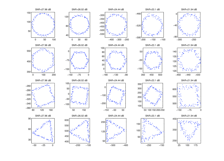
Figure 12: Sample test shapes. From top to bottom, the circle, the hexagon, the square, and the triangle, with varying noise level, translation, rotation, and scale factors, and point labeling. Noise increases from left to right. Note that, for high levels of noise, the shapes become difficult to distinguish, particularly the circumference and the hexagon become very similar.

We then used the classification strategy described in the previous section: our database was composed just by the ANSIGs of the four noiseless polygons and the ANSIG of each noisy test shape was classified by selecting the most similar entry in the database. We tested the classifier by performing 2000 tests for each of the four shapes, at each noisy level, obtaining 100% correct classifications for in all tests with SNR above around 28dB. Note that shapes with this level of noise are far from being visually “clean”, see the illustrations in the first column (the leftmost plots) of Fig. 12. The results are summarized in Tab. I, where we see that a few classifications errors happen for higher levels of noise, when dealing with circles or hexagons, which as noted before, for such levels of noise, are in fact difficult to distinguish, even for humans, see the rightmost plots of the first two lines of Fig. 12.

TABLE I: Percentages of correct classifications for the noisy shapes in Fig. 12.

	SNR [dB]
	$\geq$ 27.96	26.02	24.44	23.1	21.94
	100%	99.95%	99.9%	99.45%	97.3%
	100%	100%	99.9%	99.85%	99.25%
	100%	100%	100%	100%	100%
	100%	100%	100%	100%	100%

Although not the focus of this paper, we now illustrate that the ANSIG representation can also be used when dealing with non-rigid distortions, if more than one prototype per class is included in the database. We use the subset of the MPEG-7 shape database [41, 42] show in Fig. 13. It has 18 classes, each containing 12 shapes that, although perceptually similar, are not geometrically equal. We increase shape variability by creating test shapes that are noisy versions of the ones in Fig. 13 (the noise levels are illustrated with an example in Fig. 14).

Figure 13: The $216$-shape subset [42] of the MPEG-7 shape database [41], containing $12$ shape classes, each with $18$ shapes.

       

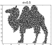
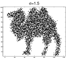
Figure 14: Illustration of the noise levels used in the MPEG-7 shape database illustrated in Fig. 13.

We stored the ANSIGs of the noiseless shapes and then classified a set of 43200 test shapes (200 for each sample shape in Fig. 13), for each of the two noise levels illustrated in Fig. 14, using a simple 1-NN classifier, i.e., selecting the class with most similar ANSIG. We got 100% correct classifications for both noise levels. See [36] for more details on this experiment and [37] for other experiment that demonstrates robustness to noise with a clip-art shape database.

V-B Real images

We now describe an experiment with real images of trademarks. We obtained from the internet a set of images of logos that are well described by its shape content. These images range from 80$\times$80 to 500$\times$500 pixels. To obtain shape vectors from intensity images, i.e., sets of points or landmarks that describe the shape content, there is a panoply of low- and mid-level processing methods that can be used, ranging from the simple image intensity threshold to sophisticated segmentation procedures. In this experiment, we just processed the images with the Canny edge detector [43] and then stored the ANSIGs of the corresponding edge maps in a database.

To test the performance of our shape recognition scheme with challenging test images, we printed the trademark images and photographed their paper version with a low quality digital camera, with different paper-camera positions, orientations, and distances. This way we obtained a set of 88 test images, where the candidate logos appear at different sizes and positions, see some examples in Fig. 15.

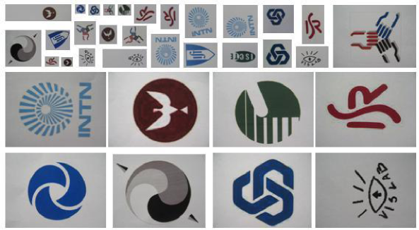
Figure 15: Examples of trademark images to be classified.

After running the Canny edge detector [43] on the test images, we performed the shape-based classification in the same way as above, i.e., by just selecting the database entry that was more similar to each test shape ANSIG. The results are summarized in Table II, in the form of a confusion matrix. We see that the generality of the test images were correctly classified. Exceptions are: one of the photographs of the fifth logo ($12.5\%$); and several photographs of the tenth one ($50\%$, $37.5\%$). In the sequel, we discuss these miss-classifications.

TABLE II: Automatic trademark retrieval experiment: confusion matrix.

	$Database$
$Photos$
	100%	0%	0%	0%	0%	0%	0%	0%	0%	0%	0%
	0%	100%	0%	0%	0%	0%	0%	0%	0%	0%	0%
	0%	0%	100%	0%	0%	0%	0%	0%	0%	0%	0%
	0%	0%	0%	100%	0%	0%	0%	0%	0%	0%	0%
	0%	0%	0%	0%	87.5%	0%	12.5%	0%	0%	0%	0%
	0%	0%	0%	0%	0%	100%	0%	0%	0%	0%	0%
	0%	0%	0%	0%	0%	0%	100%	0%	0%	0%	0%
	0%	0%	0%	0%	0%	0%	0%	100%	0%	0%	0%
	0%	0%	0%	0%	0%	0%	0%	0%	100%	0%	0%
	0%	0%	50%	37.5%	0%	0%	0%	0%	0%	12.5%	0%
	0%	0%	0%	0%	0%	0%	0%	0%	0%	0%	100%

V-C Sensitivity to model violations

We now discuss how the behavior of the ANSIG representation is affected by model violations that may arise when dealing with shapes obtained from real images. In particular, we address two kinds of model violation: failures in edge detection and perspective distortions.

Edge-detection failures. Many reasons may motivate gross failures in edge detection. For example, too many edges may be detected, due to image noise or, in opposition, too few edges may be detected, due to the absence of abrupt enough changes in the image intensity. The examples in Fig. 16 illustrate these situations. In the top left, there is one of the images in the trademark database. In the top middle and right, two test images that are photographs of the same logo. The photograph in the middle was obtained with a very large zoom (around $20\times$) and the right one was obtained in low light. Both lead to edge maps that are very distinct to the one in the database, see the plots in the bottom row of Fig. 16. The trademark images in Fig. 16 are precisely the ones that originated the miss-classifications in the tenth row of Table II. This is explained by the fact that our ANSIG representation, although invariant to permutation, translation, rotation, and scale, and robust to sampling density, can not cope, without further developments, with severe degradations such as the ones in the edge maps of Fig. 16.

           

     

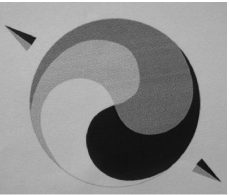
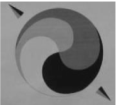
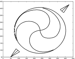
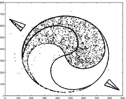
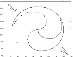
Figure 16: Failures in edge detection. Top: images; bottom: corresponding Canny edge maps [43]. Left: image in database; middle: photograph with large zoom, for which the perceived texture of the paper originates spurious edge points; bottom: photograph at low light, for which several edge points are not detected, due to less abrupt changes in image intensity.

.

Edge detection failures may also happen when processing out-of-focus photographic images. Figs. 17 and 19 present two extreme cases. For the out-of-focus test image of Fig. 17, some edge points are missed, but the corresponding ANSIG, represented in Fig. 18, results similar to the one in the database, leading to a correct classification. This is due to the robustness of the ANSIG representation in what respects to shape sampling density, recall the derivation in Section III and its illustration in Figs. 6 and 7. In opposition, the out-of-focus test image of Fig. 19 results very smooth, originating an highly incomplete edge map (compare the middle plots of Fig. 19). This is the reason for the classification error in the fifth row of Table II.

           

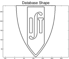
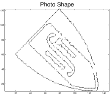
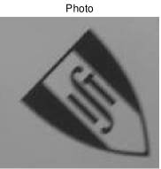
Figure 17: Recognition of an out-of-focus image. From left to right: database image, corresponding edge map, edge map of out-of-focus image, out-of-focus image. See the ANSIGs of the middle plots in Fig. 18.

         

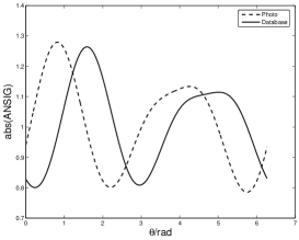
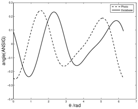
Figure 18: ANSIGs of the shapes in Fig. 17. In spite of the unfocused image that lead to the incomplete edge map, the ANSIGs are very similar (recall that the circular shift is due to different image orientation and it is easily taken care of).

           

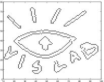
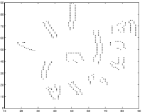
Figure 19: Failure in recognizing an out-of-focus image, due to the highly incomplete edge map.

We emphasize, however, that different pre-processing schemes may easily improve the results. In fact, one of the advantages of the shape representation scheme we propose in this paper is precisely the fact that it does not require edge segments, dealing equally well with shapes described by arbitrary sets of points. As an example, we extracted different shape vectors from the pair of images in Fig. 19, by using a simple intensity threshold, see the resulting shapes in the middle plots of Fig. 20. Since thresholding is much more insensitive to focusing effects, the shapes result more similar and the ANSIG successively captures this similarity, see Fig. 21.

           

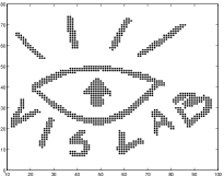
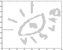
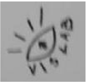
Figure 20: Comparing the same pair of images of Fig. 19, now using intensity thresholding as the pre-processing step, leads to better results. See also the ANSIGs of the middle plots in Fig. 21.

         

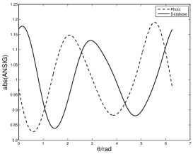
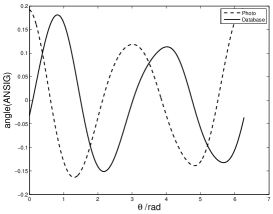
Figure 21: ANSIGs of the shapes in Fig. 20. In spite of the unfocused image, the ANSIGs are very similar (again, the circular shift is due to different image orientation and it is easily taken care of).

Perspective distortion. A different kind of model violation that may occur when dealing with 2D shapes extracted from photographic images is due to perspective distortion. In fact, while the ANSIG representation was developed assuming the shapes are 2D-rigid, this may not be the case, even when only flat objects are considered, if the camera is not adequately oriented. To illustrate the behavior of the ANSIG representation when in presence of perspective distortions, we photographed one of the trademark images, purposely from directions not perpendicular to the paper. Some of the corresponding edge maps are shown in Fig. 22, with perspective distortion increasing from left to right. The plots in Fig. 23 compare the ANSIG of the leftmost (undistorted) shape of Fig. 22 with the ANSIGs of the perspectively distorted ones. We can see that, although this effect was not taken into account in our modeling, the ANSIG representation can deal with small perspective distortions (see the similarity of the thick solid, dashed, and dot-dashed lines in the plots of Fig. 23). Naturally, when the distortions are severe, our representation fails to adequately capture the shape similarity (see the thin solid lines in the plots of Fig. 23).

                 

Figure 22: Edge maps obtained from photographs with increasing perspective distortion.

         

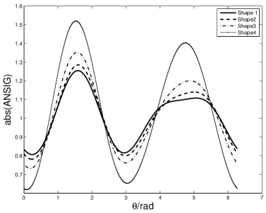
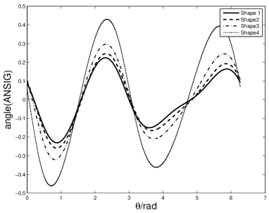
Figure 23: ANSIGs of the perspectively distorted shapes in Fig. 22.

VI Conclusion

We proposed a new method to represent 2D shapes, described by a set of unlabeled points, or landmarks, in the plane. Our method is based on what we call the analytic signature (ANSIG) of the shape, whose most distinctive characteristic is its invariance to the way the landmarks are labeled. This makes the ANSIG particularly suited to cope with shapes described by large sets of edge points in images. We illustrated its performance in shape-based classification tasks.

We envisage paths for future research and development based on the ANSIG representation. In this paper, we store ANSIGs by sampling them on the unit-circle. A topic that deserves further study is not only the choice of sampling rate but also the adoption of different sampling schemes, e.g., the use of two or more concentric circles for robustness. The derivations in this paper are targeted to the representation and comparison of complete shapes. However, in many practical scenarios, it is also necessary to recognize a set of points as being a part, i.e., a subset of a given shape. A good challenge is then to adapt the ANSIG representation to deal with incomplete shapes. Finally, in our experiments, shapes are obtained directly from the (noisy) output of the edge detection process. Naturally, intermediate processing steps, e.g., the popular morphological filtering operations, would lead to “cleaner” shapes, thus to more accurate classifications.

References

- [1] I. Biederman, “Recognition-by-components: a theory of human image understanding,” Psychological Review, vol. 94, no. 2, pp. 115–147, 1987.
- [2] D. Mumford, “Mathematical theories of shape: do they model perception ?” in Proc. of the SPIE Conf. on Geometric Methods in Computer Vision, San Diego CA, USA, 1991.
- [3] L. Schomaker, E. Leau, and L. Vuurpijl, “Using pen-based outlines for object-based annotation and image-based queries,” in Proc. of the Int. Conf. on Visual Information and Information Systems, Amsterdam, The Netherlands, 1999.
- [4] C. Small, The Statistical Theory of Shape, ser. Springer Series in Statistics. Springer-Verlag, 1997.
- [5] D. Kendall, D. Barden, T. Carne, and H. Le, Shape and Shape Theory. John Wiley and Sons, 1999.
- [6] M. Hu, “Visual pattern recognition by moment invariants,” IRE Trans. on Information Theory, vol. 8, pp. 179–187, 1962.
- [7] M. Teague, “Visual pattern recognition by moment invariants,” Journal of the Optical Society of America, vol. 70, pp. 920–930, 1980.
- [8] A. Khotanzad and Y. Hong, “Invariant image recognition by Zernike moments,” IEEE Trans. on Pattern Analysis and Machine Intelligence, vol. 12, pp. 489–497, 1990.
- [9] R. Mukundan, S. Ong, and P. Lee, “Image analysis by Tchebichef moments,” IEEE Trans. on Image Processing, vol. 10, pp. 1357–1364, 2001.
- [10] F. Mokhtarian and A. Mackworth, “A theory of multiscale, curvature-based shape representation for planar curves,” IEEE Trans. on Pattern Analysis and Machine Intelligence, vol. 14, no. 8, pp. 789–805, 1992.
- [11] G. Chauang and C. Kuo, “Wavelet descriptor of planar curves: Theory and applications,” IEEE Trans. on Image Processing, vol. 5, pp. 56–70, 1996.
- [12] T. Adamek and N. O’Connor, “A multiscale representation method for nonrigid shapes with a single closed contour,” IEEE Trans. on Pattern Analysis and Machine Intelligence, vol. 14, pp. 742–753, 2004.
- [13] P. Dierckx, Curve and Surface Fitting with Splines. Oxford Science Publications, 1995.
- [14] H. Kauppinen, T. Seppanen, and M. Pietikainen, “An experimental comparison of autoregressive and Fourier-based descriptors in 2D shape classification,” IEEE Trans. Pattern Analysis and Machine Intelligence, vol. 17, no. 2, 1995.
- [15] D. Zhang and G. Lu, “Study and evaluation of different fourier methods for image retrieval,” SPRINGER Int. Journal of Computer Vision, vol. 1234, pp. 33–49, 2005.
- [16] I. Bartolini, P. Ciaccia, and M. Patella, “Warp: Accurate retrieval of shapes using phase of fourier descriptors and time warping distance,” IEEE Trans. on Pattern Analysis and Machine Intelligence, vol. 27, no. 1, pp. 142–147, 2005.
- [17] A. Ghosh and N. Petkov, “Robustness of shape descriptors to incomplete contour representations,” IEEE Trans. on Pattern Analysis and Machine Intelligence, vol. 27, no. 11, pp. 1793–1804, 2005.
- [18] S. Belongie, J. Malik, and J. Puzicha, “Shape matching and object recognition using shape contexts,” IEEE Trans. on Pattern Analysis and Machine Intelligence, vol. 24, no. 24, pp. 509–522, 2002.
- [19] C. G. N. Petkov, “Distance sets for shape filters and shape recognition,” IEEE Trans. on Image Processing, vol. 12, no. 10, pp. 1274–1286, 2003.
- [20] P. Besl and N. McKay, “A method for registration of 3-D shapes,” IEEE Trans. on Pattern Analysis and Machine Intelligence, vol. 14, no. 2, 1992.
- [21] H. Chui and A. Rangarajan, “A new algorithm for non-rigid point matching,” in Proc. of IEEE Int. Conf. on Computer Vision and Pattern Recognition, Hilton Head Island, South Carolina, USA, 2000.
- [22] B. Luo and E. Hancock, “Iterative procrustes alignment with the EM algorithm’,” ELSEVIER Image and Vision Computing, vol. 20, pp. 377–396, 2002.
- [23] J. Kent, K. Mardia, and C. Taylor, “Matching problems for unlabelled configurations,” in Proceedings of the Int. Conf. on Bioinformatics, Images, and Wavelets, R. Aykroyd, S. Barber, and U. o. L. K. Mardia, Eds., Leeds, UK, 2004.
- [24] G. McNeill and S. Vijayakumar, “Part-based probabilistic point matching using equivalence constraints,” in Proc. of the Annual Conf. on Neural Information Processing Systems, Vancouver BC, Canada, 2006.
- [25] ——, “A probabilistic approach to robust shape matching,” in Proc. of the IEEE Int. Conf. on Image Processing, Atlanta GA, USA, 2006.
- [26] ——, “Hierarchical procrustes matching for shape retrieval,” in Proc. of the IEEE Int. Conf. on Computer Vision and Pattern Recognition, New York NY, USA, 2006.
- [27] G. McLachlan and T. Krishnan, The EM Algorithm and Extensions. New York: John Wiley & Sons, 1997.
- [28] T. Jebara, “Images as bags of pixels,” in Proc. of the IEEE Int. Conf. on Computer Vision, Nice, France, 2003.
- [29] ——, “Convex invariance learning,” in Proc. of Int. Conf. on Artificial Intelligence and Statistics, Key West FLA, USA, 2003.
- [30] ——, “Kernelizing sorting, permutation and alignment for minimum volume PCA,” in Proc. of Annual Conf. on Learning Theory, Banff, Alberta, Canada, 2004.
- [31] P. Shivaswamy and T. Jebara, “Permutation invariant SVMs,” in Proc. of Int. Conf. on Machine Learning, Pittsburgh PA, USA, 2006.
- [32] R. Kondor, A. Howard, and T. Jebara, “Multi-object tracking with representations of the symmetric group,” in Proc. of Int. Conf. on Artificial Intelligence and Statistics, San Juan, Puerto Rico, 2007.
- [33] M. Boutin and G. Kemper, “On reconstructing -point configurations from the distribution of distances of areas,” ELSEVIER Advances in Applied Mathematics, vol. 32, pp. 709–735, 2004.
- [34] K. Lee, M. Boutin, and M. Comer, “Lossless shape representation using invariant statistics: the case of point sets,” in Proc. of Asilomar Conf. on Signals, Systems, and Computers, Pacific Grove CA, USA, 2006.
- [35] M. Boutin and M. Comer, “Faithful shape representation for 2D gaussian mixtures,” in Proc. of IEEE Int. Conf. on Image Processing, San Antonio TX, USA, 2007.
- [36] J. Rodrigues, P. Aguiar, and J. Xavier, “ANSIG – an analytical signature for permutation-invariant two-dimensional shape representation,” in Proc. of IEEE Int. Conf. on Computer Vision and Pattern Recognition, Anchorage, Alaska, USA, 2008.
- [37] J. Rodrigues, J. Xavier, and P. Aguiar, “Classification of unlabeled point sets using ANSIG,” in Proc. of IEEE Int. Conf. on Image Processing, San Diego, CA, USA, 2008.
- [38] R. Horn and C. Johnson, Matrix Analysis. Cambridge, UK: Cambridge University Press, 1985.
- [39] L. Ahlfors, Complex Analysis. New York, USA: McGraw-Hill, 1978.
- [40] A. Oppenheim, R. Schafer, and J. Buck, Discrete-Time Signal Processing. Prentice Hall, 1999.
- [41] L. J. Latecki, R. Lakamper, and U. Eckhardt, “Shape descriptors for nonrigid shapes with a single closed contour,” in Proc. of IEEE Int. Conf. on Computer Vision and Pattern Recognition, Hilton Head Island, SC, USA, 2000.
- [42] T. Sebastian, P. Klein, and B. Kimia, “Recognition of shapes by editing their shock graphs,” IEEE Trans. on Pattern Analysis and Machine Intelligence, vol. 26, no. 5, pp. 550–571, 2004.
- [43] J. Canny, “A computational approach to edge detection,” IEEE Trans. on Pattern Analysis and Machine Intelligence, vol. 8, pp. 679–714, 1986.