Quantum Tunneling and Scattering of a Composite Object:
Revisited and Reassessed

Abstract

This work presents an extensive exploration of scattering and tunneling involving composite objects with intrinsic degrees of freedom. We aim at exact solutions to such scattering problems. Along this path we demonstrate solution to model Hamiltonians, and develop different techniques for addressing these complex reaction-physics problems, discuss their applicability, and investigate the relevant convergence issues. As examples, we study the scattering of a two-constituent deuteron-like systems either with an infinite set of intrinsic bound states or with a continuum of states that allows for breakup. We show that the internal degrees of freedom of the projectile and its virtual excitation in the course of reactions play an important role in shaping the S-matrix and related observables, giving rise to enhanced or reduced tunneling in various situations.

I Introduction

Reaction physics involving composite objects is a major and critical subject while encountered in the context of processes like fusion, fission, particle decay, as well as specific branches of science including chemistry, atomic physics, condensed matter physics, etc. In all these phenomena, more often than not, the scattering or tunneling object has its own degrees of freedom. Various pertinent scenarios have been explored earlier, where the tunneling has been shown to be enhanced by the additional degree(s) of freedom, which may have arisen from the compositeness of the object Flambaum and Zelevinsky (2005); Bertulani et al. (2007); Balantekin and Takigawa (1998); Bonini et al. (1999); Goodvin and Shegelski (2005); Saito and Kayanuma (1994); Bacca and Feldmeier (2006), from its interaction with another particle Ivlev and Gudkov (2004), or directly from quantum field excitations Flambaum and Zelevinsky (1999).

This is a complicated and generally non-perturbative problem, involving vastly different scales. While there are many techniques and methods of dealing with this problem, most of them involve simplifications. For example, some studies of the models that are similar to ours involve restriction on the range of energy of the projectile Bertulani et al. (2007), the mass-ratio of the constituents Bertulani et al. (2007); Goodvin and Shegelski (2005); Saito and Kayanuma (1994); Bacca and Feldmeier (2006), the number of states available in the intrinsic system Goodvin and Shegelski (2005); Bacca and Feldmeier (2006), etc. In addition, most models exclude the possibility of virtual excitations of the object undergoing a reaction Flambaum and Zelevinsky (2005); Goodvin and Shegelski (2005); Bacca and Feldmeier (2006). While simplifications work well at times, it is also common that the “slightly simplified” problem turns out to be very different from the original one. Moreover, some formally exact techniques, as demonstrated in Ref. Ahsan and Volya (2010) and further discussed in this paper, do not necessarily provide a path to a convergent solution for an arbitrary subset of parameters. The paramount goal of this work is to find an exact solution to a given reaction problem, which is free from the above mentioned limitations and is reliably convergent.

In order to reach this goal we limit our studies specifically to a problem in one dimension and to a composite object with two constituents, only one of which interacts with an external potential. A deuteron hitting a Coulomb barrier could be a fair example of such a projectile. This picture has been modeled in several different ways in our work. However, the techniques that we develop and the study of how they work are general and are not limited, in their applicability, to our examples or models only. Moreover, we believe that many of our findings are generic and there are realistic situations that can be represented by even these simple models Lemasson et al. (2009).

Our discussion is organized as follows. In Sec. II we start by identifying our models and invoking some definitions of reaction physics. Then in Sec. III we examine a particularly simple example of a deuteron-like system reflecting from an infinite wall. This case provides an excellent illustration of the pivotal role of virtual excitations in the dynamics. It also shows how the formally exact method of projecting the reaction dynamics onto the intrinsic shell-model-like space could fail to yield reliable results. We put forward and demonstrate the Variable Phase Method (VPM) in Sec. IV, followed by solutions to various examples in Sec. V. While the VPM has been used by others in the past, we extend it so as to include virtual channels. This novel extension requires us to explore the role of virtual channels and to discuss the convergence of solutions with the number of virtual excitations included in consideration. This is done in Sec. VI. A study of scattering and breakup of a system with a continuum of states is presented in Sec. VII. The summary and conclusions are laid out in Sec. VIII.

II General Description of the Problem

II.1 The model

Throughout this text we examine a one-dimensional problem. We consider a projectile which is a composite object made up of two particles which have masses $m_{1}$ and $m_{2}$ and are bound by an intrinsic potential $v(x_{1}-x_{2})$, where the particle coordinates are $x_{1}$ and $x_{2}$, respectively. This composite system interacts with an external potential $V(x_{1},x_{2})$. The usual center-of-mass and relative coordinates are

$$X=\frac{m_{1}x_{1}+m_{2}x_{2}}{M}\,,\qquad x=x_{1}-x_{2},$$ (1)

and the corresponding total and reduced masses are

$$M=m_{1}+m_{2},\qquad m=\frac{m_{1}m_{2}}{m_{1}+m_{2}}.$$ (2)

The Hamiltonian for the system can be written as

$$H=-\frac{\hbar^{2}}{2M}\frac{\partial^{2}}{\partial X^{2}}+V(x_{1},x_{2})+h$$ (3)

where the intrinsic Hamiltonian

$$h=-\frac{\hbar^{2}}{2m}\frac{\partial^{2}}{\partial x^{2}}+v(x)$$ (4)

has eigenstates $\psi_{n}(x)$ with the corresponding energy eigenvalues $\varepsilon_{n}$:

$$h\psi_{n}(x)=\varepsilon_{n}\psi_{n}(x),\qquad n=0,1,2,...$$ (5)

The general scattering problem can be formulated in a traditional way, using the asymptotic form of the wave function. At $X\rightarrow\mp\infty$ it is given by

$$\Phi(X,x)\simeq\frac{e^{iK_{n^{\prime}}X}}{\sqrt{|K_{n^{\prime}}|}}\psi_{n^{\prime}}(x)+\underset{n\in\mathrm{open}}{\sum}\frac{R_{nn^{\prime}}}{\sqrt{|K_{n}|}}e^{-iK_{n}X}\psi_{n}(x)\,,$$ (6a)

$$\Phi(X,x)\simeq\underset{n\in\mathrm{open}}{\sum}\frac{T_{nn^{\prime}}}{\sqrt{|K_{n}|}}e^{iK_{n}X}\psi_{n}(x)$$ (6b)

respectively. The wave function above corresponds to an incident beam coming from the left with a particle in the intrinsic state (channel) $n^{\prime}.$ Here $K_{n}$ is the center-of-mass momentum of the system with total energy $E_{T}$ while in channel $n$,

$$K_{n}(E_{T})=\frac{1}{\hbar}\sqrt{2M(E_{T}-\varepsilon_{n})}.$$ (7)

Here, and later in this paper, the symbol ‘$\simeq$’ is used to indicate an asymptotic equality that involves only open channels $n$ with $E_{T}>\varepsilon_{n}$. Contributions from the closed channels, for which $E_{T}<\varepsilon_{n}$, decay exponentially with distance from the scattering potential and are not present in the asymptotic form. The coefficients $R$ and $T$ are referred to as reflection and transmission amplitudes due to their physical meanings. $|R_{nn^{\prime}}|^{2}$ and $|T_{nn^{\prime}}|^{2}$ represent the probabilities for the incoming beam in channel $n^{\prime}$ to reflect and transmit, respectively, in channel $n.$ The conservation of probability hence implies

$$\underset{n\in\mathrm{open}}{\sum}\left(|R_{nn^{\prime}}|^{2}+|T_{nn^{\prime}}|^{2}\right)=1.$$ (8)

It should be mentioned that for the scattering problem to be fully determined one should consider, in addition to (6b), an incident beam coming from the right, which gives rise to another set of reflection and transmission amplitudes. If and when it is necessary to distinguish between these two, the amplitudes in Eqs. (6b) for the incident beam coming from the left and traveling in the positive $x$ direction are denoted by $R_{+}$ and $T_{+}$ instead of just $R$ and $T$; $R_{-}$ and $T_{-}$ are used when they are associated with an incident beam traveling from the right to the left.

II.2 The $S$-matrix

While it is convenient to use the reflection and transmission amplitudes, the formal $S$-matrix is still essential for establishing a relation between this description and the traditional scattering theory. In addition, $S$-matrix allows one to utilize the symmetries of the problem, and determine relations among the amplitudes. Despite $S$-matrix being a textbook subject Merzbacher (1998); Lipkin (1973), there are a few non-trivial features that emerge in the case of coupled-channel problems and with non-symmetric potentials Nogami and Ross (1996); Kiers and van Dijk (1996); van Dijk et al. (2008). We review some of them in what follows.

Let us first consider the case of one open channel, which is of particular importance for many examples considered in this work. For a real potential barrier the transmission amplitude is symmetric between the incoming beam traveling from the left and that from the right, which follows directly from the complex-conjugated Schrödinger equation, showing time-reversal invariance. The $S$-matrix can be defined in several different ways Nogami and Ross (1996). It is quite common to select a basis with incoming and outgoing waves so that $S=\mathbf{1}$ at high energies or in the absence of a potential barrier. An alternative approach is to choose the $S$-matrix to be symmetric, which is possible because of the time-reversal invariance. Unfortunately, it is impossible to accommodate both properties simultaneously. We choose the second alternative and define the $S$-matrix using the following symmetric and asymmetric (in space) asymptotic forms of the incoming waves at $|X|\rightarrow\infty$,

$$\Phi^{+}(X)\simeq\frac{i}{\sqrt{2}}\exp\left(-iK|X|\right)\,\,{\rm and}$$

$$\Phi^{-}(x)\simeq\frac{i}{\sqrt{2}}\frac{X}{|X|}\exp\left(-iK|X|\right).$$

The outgoing-wave basis comprises the corresponding complex-conjugated wave functions. Then the $S$-matrix in terms of reflection and transmission amplitudes is

$$S=-\frac{1}{2}\left(\begin{array}[]{cc}(R_{+}+R_{-})+2T&(R_{-}-R_{+})\\ (R_{-}-R_{+})&(R_{+}+R_{-})-2T\end{array}\right).$$

Note that the S-matrix is symmetric, and $T_{+}=T_{-}=T$ due to time-reversal invariance. From unitarity of the $S$-matrix we find that $|R_{-}|=|R_{+}|,$ $|R_{\pm}^{2}|+|T_{\pm}^{2}|=1,$ and $\Re\left[T^{*}(R_{+}+R_{-})\right]=0$. The convenience with the above definition is that, for a symmetric potential, $R_{-}=R_{+}$. Also, parity is a good quantum number, and hence the $S$-matrix is diagonal with matrix elements

$$S^{\pm}=-(R\pm T)=\exp(2i\delta^{\pm}).$$ (9)

An extension of the above discussion to a more general multichannel case is straight-forward Kiers and van Dijk (1996); Baz et al. (1971). From unitarity it follows that

$$R_{\pm}^{\dagger}R_{\pm}+T_{\pm}^{\dagger}T_{\pm}={\bf 1},\quad R_{\pm}^{\dagger}T_{\mp}+T_{\pm}^{\dagger}R_{\mp}={\bf 0}.$$ (10)

Time-reversal invariance leads to

$$T_{\pm}=T_{\mp}^{T},\,R_{\pm}=R_{\pm}^{T}.$$

Finally, reflection symmetry of the scattering potential leads to $R_{+}={\cal P}R_{-}{\cal P}$ and $T_{+}={\cal P}T_{-}{\cal P}$. The equalities for one channel are modified due to the different parities of the intrinsic states of the composite object. ${\cal P}$ denotes the parity operator in the channel space, so that ${\cal P}^{2}={\bf 1}$ with ${\cal P}_{nn^{\prime}}=\delta_{nn^{\prime}}\pi_{n}$, where $\pi_{n}$ is the parity of the intrinsic state $\psi_{n}(x)$.

In the presence of reflection symmetry it is sufficient to consider only beams originating from the left and thus to deal only with $R_{+}$ and $T_{+}$. From this point onward we omit the subscript $+$ (hence returning to the notations used in Eqs. (6b). The symmetries discussed for the multichannel case are summarized as follows:

$$R=R^{T},\quad T={\cal P}T^{T}{\cal P},$$ (11)

$$R^{\dagger}R+T^{\dagger}T={\bf 1},\quad R^{\dagger}{\cal(P}T)+(PT)^{\dagger}R={\bf 0}.$$ (12)

We define

$$S^{\pm}=-(R\pm{\cal P}T)$$ (13)

in this case, so that the $S$-matrix is symmetric, and the phase shifts approach zero in the limit of zero energy, since $R=-1$ and $T=0$ in this limit. Conditions at other thresholds are related to Levinson’s theorem which, for one-dimensional scattering, is discussed in Ref. Kiers and van Dijk (1996).

III The Projection Method: Examples and limitations

Before we actually describe the Projection Method, let us emphasize one important issue. While the observed picture (the $S$-matrix for example) is seen through the asymptotic forms of the wave functions in the open channels, the crucial dynamics of a scattering process takes place in the vicinity of the scatterer, and involves virtual (or closed) channels just as much as the open channels. The virtual channels are populated in accordance with the time-energy uncertainty, and lead to an immensely complicated process. Excluding the virtual channels from consideration could therefore lead to erroneous results in the observed quantities. A “simple” model example discussed below elucidates both the complexity and the importance of virtual excitations. This model constitutes an infinite wall as a scatterer which interacts with only one of the two constituents of the composite object. We refer to this model as the "deuteron and Coulomb-wall" model, as defined in Sec. III.1.

It is noteworthy that numerous authors Moro et al. (2000); Sakharuk and Zelevinsky (1999); Ahsan and Volya (2007), have worked on this subject, but reports of the findings are scarce. Mathematical issues, difficulties with stability of the solutions, and lack of appreciation from the scientific audience are some of the possible reasons.

In the following method, referred to as the Projection Method, a solution is attempted by projecting the reaction dynamics onto the intrinsic basis set. In some way this approach is similar to various projection techniques used in nuclear many-body studies that involve reactions Okolowicz et al. (2003); Volya and Zelevinsky (2006); Volya (2009).

We start our presentation by returning to the "deuteron and Coulomb-wall” model and to the Projection Method. We draw some conclusions regarding the earlier discussions Moro et al. (2000); Horoi et al. (1999); Sakharuk and Zelevinsky (1999); Sakharuk ; Zelevinsky ; Zelevinsky and Sakharuk (2005); Ahsan and Volya (2007) by presenting an exact solution, showing limitations of the Projection Method, and highlighting the overall importance of this example for the understanding of reaction dynamics and development of techniques.

III.1 The deuteron and Coulomb-wall model

For all the models in this work we assume that in the composite projectile, loosely referred to as the deuteron, only the second particle interacts with the potential, $V(x_{1},x_{2})\rightarrow V(x_{2})$. In this section we concentrate on an example where the potential is represented by an infinite wall or, the “wall”:

$$V(x_{2})=\begin{cases}\infty&\mathrm{\mbox{when}\;}0<x_{2}\\ 0&\mathrm{\mbox{otherwise}}\end{cases}\,.$$

The traditional textbook methods prescribe looking for a full wave function in the form

$$\Phi(X,x)=\frac{e^{iK_{n^{\prime}}X}}{\sqrt{|K_{n^{\prime}}|}}\psi_{n^{\prime}}(x)+\sum_{n}\frac{R_{nn^{\prime}}}{\sqrt{|K_{n}|}}e^{-iK_{n}X}\psi_{n}(x),$$ (14)

with the boundary condition $\Phi(X,x)=0$ at $x_{2}=0$. In contrast to the asymptotic form in (6b), where the summation includes open channels only, the sum here is over all channels and the expression holds for all values of $x_{2}<0$. The meaning of the reflection amplitudes $R_{nn^{\prime}}$ is therefore extended to include the virtual channels as well as open. The asymptotic form (6b) is recovered at $|X|\rightarrow\infty$ because the term corresponding to each virtual channel, say $n$, decays with distance (from the wall) through the exponential factor $e^{-|K_{n}X|}$, and therefore does not appear in the asymptotic sum. This exponent can be expressed in a generic way as $e^{iK_{n}|X|}$ by assuming the principal branch of the square root in Eq. (7). The branch being specified allows one to consider momentum in a complex plane.

The location $x_{2}=0$ in the boundary condition translates into $x=x_{1}$ and $X=\mu_{1}x$, as follow from Eqs. (1). Here we define relative masses as

$$\mu_{1,2}=m_{1,2}/M,\quad\mathrm{and}\quad\mu=m/M.$$ (15)

Thus, the equation to be solved is

$$\Phi(\mu_{1}x,\,x)=0$$ (16)

for all $x$’s.

The length scale for this problem is determined by a quantity $\lambda$ that is associated with the characteristic width of the intrinsic potential $v(x)$. The intrinsic system also defines the energy scale, based on the usual coordinate-momentum uncertainty, as

$$\epsilon=\frac{\hbar^{2}}{2m\lambda^{2}}.$$ (17)

In what follows we use $\lambda$ and $\epsilon$ as our units of length and energy respectively. This is equivalent to using dimensionless energy units rescaled to $\epsilon$, namely, $\varepsilon_{n}\rightarrow\varepsilon_{n}/\epsilon$ for the intrinsic energies, and ${E}\rightarrow E/\epsilon$ for the center-of-mass kinetic energy ; and lengths rescaled to $\lambda$, namely, ${x}\rightarrow x/\lambda$, $X\to X/\lambda$ and ${K}_{n}\rightarrow K_{n}\lambda$ for coordinate and momentum variables. Thus, it is assumed that $\lambda=1$ and $\epsilon=1$ unless otherwise stated. The center-of-mass kinetic energy for an incident beam in channel $n$ is $E=E_{T}-\varepsilon_{n}$; in almost all our examples the incident beam is in the ground state channel, and therefore $n=0$.

Truncating the number of channels at some large $N$ and looking for a solution in the space spanned by the functions $\psi_{n}$ for $n<N$ constitutes the projection approach. Thence emerge the equations

$$\sum_{n}\frac{D_{ln}\left[-i\mu_{1}({K}_{n^{\prime}}+{K}_{n})\right]}{\sqrt{|{K}_{n}|}}\,R_{nn^{\prime}}=-\frac{\delta_{ln^{\prime}}}{\sqrt{|{K}_{n^{\prime}}|}}\,,$$ (18)

where matrix $D$ is defined as

$$D_{ln}(\varkappa)=\int\psi_{l}^{*}(x)\>e^{\varkappa{x}}\>\psi_{n}(x)\,dx.$$ (19)

This is the expectation value of the momentum shift operator in the intrinsic basis. Eq. (18) is obtained by projecting the boundary condition onto the intrinsic basis set. Note that for a virtual channel, the argument of the $D$-matrix becomes real and positive.

At beam energies below the first threshold, when only the ground state channel ($n=0$) is open, Eq. (16) is particularly simple, since scattering is characterized by only a single phase of the reflection amplitude. Due to unitarity $|R_{00}|=1$; and the single $S$-matrix phase $\delta$ is defined through $e^{2i\delta}=-R_{00}$. Equation (16) then reads

$$\psi_{0}({x})\,\sin\left[\mu_{1}{K}_{0}{x}-\delta\right]+\frac{1}{2}\>\sum_{n\in\mathrm{closed}}\,R^{\prime}_{n0}\sqrt{\frac{|{K}_{0}|}{|{K}_{n}|}}e^{\mu_{1}|{K}_{n}|\,{x}}\psi_{n}({x})=0,$$ (20)

where $R^{\prime}_{n0}=R{}_{n0}e^{-i(\delta+\pi/2)}$ is real for any $n$.

To further illustrate the situation let us review two specific examples of intrinsic potential $v(x)$ where the eigenstates (5) and the shift matrices (19) can be found analytically.

III.1.1 Infinite square well ("well”) confinement

In the first example, which is that of an infinitely-deep square well intrinsic confinement, the length scale $\lambda$ is defined so as to set the width of the well to $\pi\lambda$, thus

$$v(x)=\begin{cases}0&\mathrm{\mbox{when}\;}|x|<\pi\lambda/2\\ \infty&\mathrm{\mbox{otherwise}}\end{cases}\,.$$ (21)

The eigenstates and the corresponding energies for this square well are

$$\psi_{n-1}({x})=\sqrt{\frac{2}{\pi}}\,\sin\left[\left({x}+\frac{\pi}{2}\right)n\right],\quad\varepsilon_{n-1}=n^{2}\,,$$ (22)

where $n=1,\>2,\dots$, so that the indices for both $\psi$ and $\varepsilon$ start from $0$, and the energy scale (17) is $\epsilon=\varepsilon_{0}$. The corresponding shift matrix is

$$D_{nn^{\prime}}(\varkappa)=\frac{4nn^{\prime}\varkappa\left[(-1)^{n+n^{\prime}}\exp\left(\frac{\pi\varkappa}{2}\right)-\exp\left(-\frac{\pi\varkappa}{2}\right)\right]}{\pi\left[(n+n^{\prime})^{2}+\varkappa^{2}\right]\left[(n-n^{\prime})^{2}+\varkappa^{2}\right]}.$$ (23)

III.1.2 Harmonic oscillator ("HO") confinement

One could criticize the infinite square well potential as being too sharp and therefore leading to nonphysically high intrinsic excitations. Therefore, the harmonic oscillator intrinsic confinement $v(x)=m\omega^{2}x{}^{2}/2$ is presented as a second example, which does not have this controversial feature.

The unit of length here is defined by the standard oscillator length, $\lambda=\sqrt{\hbar/m\omega}$. The eigenstates and the eigenvalues are defined in terms of the usual Hermite polynomials $H_{n}$,

$$\psi_{n}({x})=\frac{1}{\sqrt{2^{n}n!\sqrt{\pi}}}H_{n}\left({x}\right)\exp\left(-\frac{{x}^{2}}{2}\right)\,,\quad\varepsilon_{n}=(2n+1),$$ (24)

where $n=0,1,\dots$, and the energy unit is $\epsilon=\varepsilon_{0}=\frac{1}{2}\hbar\omega$. The corresponding shift matrix is

$$D_{nn^{\prime}}(\varkappa)=\sqrt{\frac{n_{<}!}{n_{>}!}}\,\left(\frac{\varkappa}{\sqrt{2}}\right)^{|n-n^{\prime}|}\,\,L_{n_{<}}^{|n-n^{\prime}|}\left(-\frac{\varkappa^{2}}{2}\right)\,\exp\left(\frac{\varkappa^{2}}{4}\right)\,,$$ (25)

where the Associated Laguerre Polynomials $L_{n}^{l}$ appear, with $n_{<}$ and $n_{>}$ denoting the smaller and larger, respectively, of the two indices $n$ and $n^{\prime}$.

III.2 Solutions, difficulties, and limitations

From the explicit forms of the shift matrices in the two cases described in Eqs. (23) and (25), it is clear that the shift matrix in Eq. (18), when inverted, has highly singular elements for $N\rightarrow\infty$. To be precise, $\varkappa_{n}\sim n\sqrt{m_{1}/m_{2}}$ for a square well (and $\varkappa_{n}\sim\sqrt{2nm_{1}/m_{2}}$ for oscillator) which implies that the elements in Eq. (19) of the shift-matrix have exponentially different scales.

This difficulty of matrix inversion can be handled by performing a linear transformation from the set of basis states $\psi_{n}(x)$ to a different set. Transformation to configuration localized state is discussed in Ref. Moro et al. (2000). In our studies we used the singular value decomposition which is also effective. As was observed in Refs. Horoi ; Sakharuk and Zelevinsky (1999); Sakharuk ; Zelevinsky ; Zelevinsky and Sakharuk (2005), there are complications in numerical convergence with an increased number $N$ of included channels. The core of the problem is that the amplitudes for real and virtual channels involve very different scales. We find that for the square well, for example, remote virtual channels scale approximately as $R_{n}=R_{n0}\sim\exp\left[\frac{\pi n}{2}\sqrt{\frac{m_{1}}{m_{2}}}\right]$ (similar scaling follows for the oscillator). The behavior of the virtual coefficients is illustrated in Fig. 1. Here and in what follows, the second index in $R_{nn^{\prime}}$ and $T_{nn^{\prime}}$, which corresponds to the incident channel, is dropped when it is the ground state channel, i.e., when $n^{\prime}=0$.

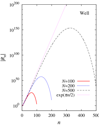
Figure 1: (Color online) Well and wall. Absolute values of reflection amplitudes for virtual channels are plotted against channel number $n$. The infinite square well potential (intrinsic) is used in this example, with $m_{1}=m_{2}$. The incident beam is in the ground state with kinetic energy $E=0.1$. Different curves correspond to different truncations $N$. The straight line shows the curve $\exp(\pi n/2)$. The actual results closely follow this line initially and then deviate due to truncation in the channel space.

As the physics of interest is comprised of small contributions from exponentially large excitations, the problem has mathematical issues. This is apparent also from Eqs. (16) and (20), where one is attempting to make a series with exponentially divergent coefficients vanish. This condition fails to fulfill especially for large mass-ratios $m_{1}/m_{2}$, when the coordinate-range $|x|\sim\lambda$ (where $\psi_{n}$ are not zero) implies large exponential factors $e^{|K_{n}|\lambda\mu_{1}}$. The physics behind this is that when the interacting particle is stopped by the wall, the non-interacting component continues its motion until its entire kinetic energy is converted into virtual intrinsic excitations of the confining potential which is necessary for the system to be reflected. The bigger the mass of the non-interacting particle $m_{1}$ relative to $m_{2}$, the more kinetic energy it has, and the more complicated do the virtual excitations become. Figure 2 shows how this issue effects calculated results.

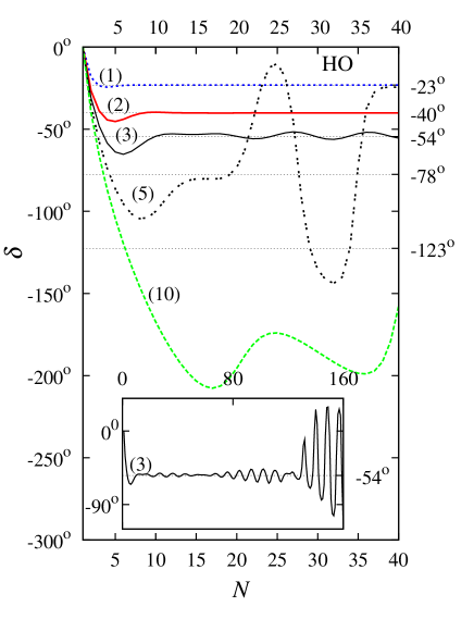
Figure 2: (Color online) HO and wall. This plot demonstrates the failure of the Projection Method, which uses Eq. (18), to solve the scattering problem where the system of two particles bound by a harmonic oscillator confinement collides with an infinite wall. The incident kinetic energy is $E=1=0.5\,\hbar\omega$, which means that the total energy is half way between those of the ground state and of the first excited state. Different curves are labeled on the graph with the corresponding mass-ratios, $m_{1}/m_{2}=$ 1, 2, 3, 5, and 10. Phase shift $\delta$ is shown to vary with $N$, the number of channels included in the calculation. The horizontal grid lines along with the tic-marks on the right indicate the values of the phase shifts, as obtained in a convergent way with a different method, the VPM (see Sec. IV). The curve for $m_{1}/m_{2}=3$ on a large scale up to $N=160$ is shown in the inset.

For “good” mass-ratios, which is roughly when $m_{1}/m_{2}\leq 2$, reliable solutions can be obtained Moro et al. (2000); Ahsan and Volya (2007) that agree with exact and stable solutions gotten through a different method (the VPM, see Sec. IV), as shown in Sec. V.2. For these satisfactory results, the Projection Method had to involve arbitrary-precision numerics ensuring that both the small and the large contributions are properly taken care of. The reflection probabilities in different open channels calculated for the square well and harmonic oscillator models with $m_{1}/m_{2}=1$ are reliable. They are also identical to those obtained through the VPM, and are shown in Figs. 14 and 15, respectively, in Sec. V.2. These two figures display cusps at thresholds, which is a consequence of unitarity Landau and Lifshitz (1981); Baz et al. (1971). In addition to that, there are weak oscillations which, as discussed in the same section, become more pronounced in the case of a more massive non-interacting particle.

The solution, however, is still elusive. This is especially visible for “bad” mass-ratios with large values of $m_{1}/m_{2}$. The Projection Method results are shown in Fig. 2. As the mass of the non-interacting particle $m_{1}$ gets larger, the results become extremely unstable. While a satisfactory value may be obtained for some cases, the approach is still flawed since the inclusion of more channels (which must be accompanied by increased numerical precision) does not necessarily improve the results and may eventually lead to increasing oscillatory instabilities. This is demonstrated in the inset where the curve (3) for $m_{1}/m_{2}=3$, which seems to converge initially, is continued up to N=160 where its behavior becomes erratic.

In order to solve this problem, one should depart from projection onto the basis states. In what follows this is achieved by introducing a Variable Reflection Amplitude $U_{nn^{\prime}}(X)$ (see Ref. Razavy (2003)) through the following equation,

$$R_{nn^{\prime}}=e^{i(K_{n}+K_{n^{\prime}})X}\left[2i\sqrt{K_{n}K_{n^{\prime}}}\,U_{nn^{\prime}}(X)-\delta_{nn^{\prime}}\right].$$ (26)

Then Eq. (16) takes the form

$$\sum_{n}U_{nn^{\prime}}(\mu_{1}x)\psi_{n}(x)=0,$$

and can be efficiently solved by selecting a discrete set of $N$ coordinate locations. This is the essence of a different approach discussed next.

IV The Variable Phase Method (VPM)

It follows from the discussion in the previous section that the approach based on projection onto the intrinsic basis is unpredictable in its ability to handle the problem. As an alternative, the time-dependent methods have previously been used to treat similar problems van Dijk et al. (2008). Here we discuss the Variable Phase Method (VPM), which is a well established technique for treating multi-channel tunneling and scattering. It dates back to works presented in Refs. Morse and Allis (1933); Drukarev (1949); Kynch (1952); Calogero (1963); Calogero and Ravenhall (1964); Babikov (1967); Tikochinsky (1970). Exhaustive treatises on the subject are found in books by Razavy Razavy (2003), Babikov Babikov (1968), and Calogero Calogero (1967). Solving differential equations for the phases of the stationary-state wave functions, as functions of coordinate, is central to the VPM approach. These phases at asymptotic distances (from the scattering potential) make up the $S$-matrix of the problem. Equations for such quantities can be found by considering the phase shifts corresponding to the scattering potential being truncated at some coordinate locations. Alternatively, Green’s function approach can be used. Techniques of this sort are widely used in reaction physics with atoms, molecules, and nuclei, and in relativistic scattering. Recently, there have been interests centered around multi-channel tunneling and scattering problems Goodvin and Shegelski (2005); Balantekin and Takigawa (1998); Saito and Kayanuma (1994); Razavy (2003); Hnybida and Shegelski (2008); Shegelski et al. (2008a, b). Our problem is unlike those ordinarily encountered because its solution depends on proper treatment of the multi-channel virtual dynamics. Thus, here we enhance the VPM by applying it to virtual channels, which is mentioned in Ref. Babikov (1968) as a possibility. Some later steps in this direction have been taken in Ref. Talukdar et al. (1981) with off-shell amplitudes in the context of a three-body problem.

IV.1 Formulation of the VPM

Let us first introduce the VPM briefly. We would like to emphasize that though we limit our discussion to one-dimensional scattering for simplicity, the approach is a general one. This method is also known as the Variable Reflection Amplitude Method Kiers and van Dijk (1996); Razavy (2003); Tikochinsky (1977). By using factorization of the form

$$\Phi(X,x)=\sum_{n}\Psi_{n}(X)\psi_{n}(x)$$

for the wave function, Schrödinger’s equation $H\Phi(X,x)=E_{T}\Phi(X,x)$ with the Hamiltonian from (3)-(4) can be transformed into a coupled-channel equation for the center-of-mass wave-functions $\Psi_{n}(X)$ for channels $n$ (subject to appropriate boundary conditions)

$$\left[\frac{\partial^{2}}{\partial X^{2}}+K_{n}^{2}\right]\Psi_{n}(X)-\sum_{n^{\prime}}V_{nn^{\prime}}(X)\Psi_{n^{\prime}}(X)=0,$$ (27)

where the folded potentials are

$$V_{nn^{\prime}}(X)=\frac{2M}{\hbar^{2}}\int_{-\infty}^{\infty}\psi_{n}^{*}(x)\,V(X,x)\,\psi_{n}(x)dx\,,$$ (28)

and $K_{n}$ is defined in Eq. (7).

The reflection and transmission amplitudes are specified in reference to the potential-free solutions of Schrödinger’s equation. These solutions are defined in terms of diagonal matrices as

$$\Xi_{nn^{\prime}}^{\pm}(X)=\frac{e^{\pm iK_{n}X}}{\sqrt{-2iK_{n}}}\,\delta_{nn^{\prime}},$$ (29)

where the $\pm$ sign corresponds to a wave moving in the right/left direction. These solutions are normalized to unit current with the Wronskian set to unity,

$$\Xi^{+}(X)\frac{d\Xi^{-}(X)}{dX}-\Xi^{-}(X)\frac{d\Xi^{+}(X)}{dX}=1.$$

The functions defined in (29) can be used for both open and closed channels provided that, as mentioned earlier, the principal branch of the square-root is selected for an imaginary $K_{n}$.

While there are variations of the VPM technique Razavy (2003), we demonstrate here the approach that explicitly emphasizes the decoupling of the reflection and transmission coefficients and the different roles thereof Babikov (1968).

It is convenient to apply the VPM by considering an auxiliary set of free-space wave functions

$$\Psi(X,X^{\prime})=\left[\Xi^{+}(X)+\Xi^{-}(X)\,R(X^{\prime})\right]\overline{T}(X^{\prime})$$ (30)

with coefficients $R(X^{\prime})$ and $\overline{T}(X^{\prime})$ defined from the solution $\Psi(X)$ of Schrödinger’s Eq. (27), using the Cauchy boundary condition at some point $X^{\prime},$ so that at $X=X^{\prime}$

$$\Psi(X,X^{\prime})=\Psi(X)\quad\mathrm{and}\quad\frac{d}{dX}\Psi(X,X^{\prime})=\frac{d}{dX}\Psi(X).$$ (31)

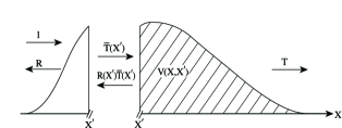
Figure 3: An incoming wave of amplitude $1$ is traveling from the left toward the potential barrier. It is reflected with amplitude $R$ and transmitted with amplitude $T$. For any arbitrary point $X^{\prime}$ the barrier is thought of as a combination of two parts: the unshaded part to the left of $X^{\prime}$, and the shaded part $V(X,X^{\prime})$ to the right. At $X^{\prime}$, in accordance with Eqs. (30) and (31), the incoming and outgoing components are identified as having amplitudes $\overline{T}(X^{\prime})$ and $R(X^{\prime})\overline{T}(X^{\prime})$ respectively. Here $\overline{T}(X^{\prime})$ represents the overall amplitude of the wave function at $X^{\prime}$ which has been modified, relative to the incoming beam, due to the passage through the unshaded part of the barrier. In the context of the shaded part only, $\overline{T}(X^{\prime})$ represents an incident beam normalization; thus $R(X^{\prime})$ is interpreted as the amplitude of reflection from the shaded part. Due to this normalization, the transmission amplitude $T(X^{\prime})$ through the shaded part is given by the final amplitude $T$ (transmission through the full potential) normalized relative to the incident amplitude $\overline{T}(X^{\prime}).$ Thus, $T(X^{\prime})\,\overline{T}(X^{\prime})=T.$ The incoming beam has a unit amplitude, and $\overline{T}(-\infty)=1,\quad T(-\infty)=T.$ It is obvious that $R(-\infty)=R$ which is the amplitude of reflection from the full potential. On the right of the potential $R(\infty)=0,\quad\overline{T}(\infty)=T,$ and $T(\infty)=1.$

It is convenient to interpret $\Psi(X,X^{\prime})$ for $X\leq X^{\prime}$ as the wave function corresponding to a potential truncated from the left, $V_{nn^{\prime}}(X,X^{\prime})=V_{nn^{\prime}}(X)\,\theta(X-X^{\prime})$, where $\theta(X)$ is the Heaviside step function. So, $V_{nn^{\prime}}(X,X^{\prime})=0$ at $X\leq X^{\prime}$, and the wave function is given by (30) with the boundary condition (31). This interpretation is illustrated in Fig. 3. Now, $R(X^{\prime})$ in (30) is a matrix in the channel space. With the help of Fig. 3, it can be identified as the reflection amplitude for a wave scattering from the potential truncated from left (the shaded part in the figure). The vector $\overline{T}(X^{\prime})$ in the channel space is the amplitude of the wave function $\Psi(X,X^{\prime})$ at $X=X^{\prime}$. It can be normalized in different ways. In the literature the wave function $\Psi$ and its amplitude $\overline{T}$ are commonly viewed as collections of independent column vectors corresponding to different independent initial conditions (initial channels). It is clear from Fig. 3 that transmission through the potential $V(X,X^{\prime})$ is inversely proportional to the amplitude $\overline{T}(X^{\prime})$. With relatively straight-forward derivations that involve substitution of the wave function in Schrödinger’s Eq. (27) by (30) (see also Ref. Babikov (1968)), one can show that the matrix $R(X)$ is subject to the differential equation

$$\frac{dR(X)}{dX}=\left[\left(\Xi^{+}+R(X)\,\Xi^{-}\right)\right]V\left[\Xi^{+}+\Xi^{-}\,R(X)\right].$$ (32)

The $X$-dependency of the $\Xi$’s and the folded potential $V$ is suppressed in this differential equation and all others to follow unless there is an ambiguity.

The equation for the vector $\overline{T}(X)$ is linear,

$$\frac{d\overline{T}(X)}{dX}=-\Xi^{-}\,V\,\left[\Xi^{+}+\Xi^{-}\,R(X)\right]\overline{T}(X),$$ (33)

which reflects linearity of quantum mechanics. To be more specific, the linearity shows that the column-vectors corresponding to different initial channels are independent of each other, and the amplitudes allow for arbitrary normalizations.

The reaction physics of interest, in agreement with the discussion in Sec. II.2, is given by $R$ alone; and, the physical properties are independent of normalization, resulting in the decoupled equation (32) for $R(X)$.

As follows from the boundary condition on the wave function $\Psi(X)$ or from the interpretation of $R(X^{\prime})$ as a reflection amplitude, $R(X^{\prime})$ is subject to the boundary condition

$$R_{nn^{\prime}}(\infty)=0,\quad\mathrm{\mathrm{that\,}leads\,to}\quad R_{nn^{\prime}}(-\infty)=R_{nn^{\prime}}.$$ (34)

The transmission amplitude is determined by $\overline{T}(X^{\prime})$. One can treat $\overline{T}(X^{\prime})$ as a matrix of the column-vectors described previously. Assuming the incident beam to be in channel $n^{\prime}$ and normalizing it to unity (which is the most common and natural way), one would have

$$\overline{T}{}_{nn^{\prime}}(-\infty)=\delta_{nn^{\prime}},\quad\mathrm{and}\,\mathrm{thus,\quad}\overline{T}_{nn^{\prime}}(\infty)=T_{nn^{\prime}}\,.$$ (35)

The elements of the reflection matrix $R(X)$ are sufficient to determine all observable probabilities. One, however, may still want to obtain the transmission amplitudes, which can be done by integrating Eq. (33) separately using previously determined values of $R(X)$. Due to the different boundary conditions for $R$ and $T$ (see Eqs. (34) and (35)), this approach is computationally inconvenient. However, given that $\overline{T}{}_{nn^{\prime}}(\infty)=T_{nn^{\prime}}$, it can be interpreted as a final state normalization to a yet-unknown value $T_{nn^{\prime}}$, and this inconvenience can be avoided. If one defines a matrix $T(X)$ so that $T(X)\overline{T}(X)=T$. Then $T(X)$ coincides exactly with the matrix of transmission amplitudes through the truncated potential $V(X,X^{\prime})$ (see Fig. 3). Since $\frac{d}{dX}(T(X)\overline{T}(X))=0$, Eq. (33) in terms of $T(X)$ is

$$\frac{dT(X)}{dX}=T(X)\,\Xi^{-}\,V\,\left[\Xi^{+}+\Xi^{-}\,R(X)\right].$$ (36)

It is to be used with the boundary condition

$$T_{nn^{\prime}}(\infty)=\delta_{nn^{\prime}},\quad\mathrm{and\>then}\quad T_{nn^{\prime}}(-\infty)=T_{nn^{\prime}}\,.$$ (37)

This approach is equivalent to the one discussed in Ref. Razavy (2003).

In summary, the most celebrated advantages of the VPM are its physical transparency, generality, and the simplicity in its application. Phase equations can indeed be constructed for most quantum mechanical problems. In particular, with appropriate substitutions for the $\Xi^{\pm}$ functions, the approach can be immediately used in three dimensional problems with radial variables. The VPM is technically simple; the entire multi-channel problem is reduced to a relatively straight-forward integration of Riccati equation (32) from right to left with a zero starting-value (for $R(X)$) as a boundary condition.

IV.2 Virtual channels in the VPM

In this work we find yet another value of the VPM in its effectiveness in treating virtual channels and in general complex-momentum (i.e., off-shell) applications. Some suggestions, in this direction, have been made in Refs. Babikov (1968); Talukdar et al. (1981). However, there are a few important things to note:

First, the formalism remains valid in the complex momentum plane assuming that for virtual channels the principal branch of the square root is selected in Eq. (7).

Secondly, separation of the amplitude (given by $\overline{T}(X)$) from the physically relevant phase difference between incoming and outgoing components (given by $R(X)$) is important. Due to this separation, the principal equation (32) is solved with a zero-value boundary condition (34), and without any concern about exponentially falling or rising components of the wave function outside the potential. Normalization is provided by a set of decoupled equations for each selected initial condition. Therefore, while solving scattering problems, one could consider only those columns $\overline{T}(X)$ that correspond to open channels of interest.

Closed channels can be studied, if desired, with an initial wave function exponentially rising toward the potential. Bound states can also be explored in this way Calogero (1967), but we do not study these questions.

Normalizing in a way to have the closed channels set to zero still deserves some attention. As further demonstrated in Sec. V.1.1, $T(X)$ and $\overline{T}(X)$ for closed channels are set to zero differently. For $\overline{T}(X)$ one assumes the initial beam normalization of zero for any closed channel, i.e.,

$$\overline{T}_{nn^{\prime}}(-\infty)=0\qquad\mathrm{if\>}n^{\prime}\>\mathrm{is\>closed}.$$ (38)

Thus after scattering one has waves in closed channels with amplitudes exponentially decaying to zero away from the potential.

Contrary to that, eq. (37) is best thought of as a final state normalization, thus

$$T_{nn^{\prime}}(\infty)=0\qquad\mathrm{\textrm{if\>\ n\>\ is\>\ closed}}.$$

Finally, the original Eqs. (32) and (33) used for open channels, are valid also for closed channels, but have issues with numerical stability for virtual excitations. The exponential divergence of the functions $\Xi_{nn}^{\pm}(X)$ with $n$ (or, $|K_{n}|$), especially at large $|X|$, makes it difficult to handle long-ranged potentials. We define

$$U(X)=-\Xi^{+}\Xi^{-}-\Xi^{-}\,R(X)\,\Xi^{-},$$

which agrees with Eq. (26), so that Eq. (32), written in terms of the variables $U(X)$ instead of $R(X)$, reads

$$\frac{dU_{nn^{\prime}}}{dX}=\delta_{nn^{\prime}}-i(K_{n}+K_{n^{\prime}})U_{nn^{\prime}}-\sum_{ll^{\prime}}U_{nl}V_{ll^{\prime}}U_{l^{\prime}n^{\prime}},$$ (39)

where $U$ and $V$ depend on $X$. It is noteworthy that in this form the equations no longer contain any exponential factors. A similar substitution can be done for $T(X)$ or $\overline{T}(X)$.

The amplitudes $U$ for open channels oscillate outside the potential where $V=0$, which is not the most desirable boundary condition one would want to deal with. However, this is a minor inconvenience compared to the benefit of the exponential drop of $U(X)$ for virtual channels with distance from the potential barrier. This is particularly important because in the problems that we discuss, the reaction processes contain only a few open channels but are determined by numerous closed channels.

V Applications of the VPM

V.1 A $\delta$-barrier

We proceed by considering a $\delta$-barrier as the scattering potential. Here, a bound system of two particles is incident on a potential

$$V(x_{1},\,x_{2})=\frac{\hbar^{2}}{AM}\delta(x_{2}),$$ (40)

where, again, only the second particle interacts with the potential; $A$ is a length parameter, characterizing the strength of the barrier.

Interactions of composite objects, such as diatomic molecules, with a $\delta$-barrier have been discussed before Razavy (2003); Shegelski et al. (2008a); Hnybida and Shegelski (2008), but usually without any involvement of the virtual channels and in situations where the potential-barrier acts on both the particles.

Any potential can be considered with the VPM approach in principle; however, the short-ranged $\delta$-potential provides a good way of exploring the generic features of scattering without putting efforts into computing folded-potentials. The folded potential (28) for a $\delta$-barrier (40) takes an analytic factorized form:

$$V_{nn^{\prime}}(X)=\frac{2}{\mu_{1}A}\;\psi_{n}^{*}\left(\frac{X}{\mu_{1}}\right)\;\psi_{n^{\prime}}\left(\frac{X}{\mu_{1}}\right),$$ (41)

where $\mu_{1}$ is the mass-ratio defined in (15).

In the limit of $A\rightarrow 0$ the $\delta$-barrier turns into an impenetrable wall, thus allowing us to complete the study in Sec. III, which is done in Sec. V.2.

Introduction of the short-ranged $\delta$-barrier adds just one additional length scale $A$ to the parameters used to describe the problem. There are thus three length scales in the problem, namely, the intrinsic scale $\lambda$, the incident beam wavelength $\sim 1/K$, and the potential scattering length $A.$ The corresponding energy scales are the intrinsic energy scale $\epsilon$, the incident beam kinetic energy $E$, and the energy scale associated with the $\delta$-potential, defined by

$$E_{\delta}=\frac{\hbar^{2}}{2MA^{2}}.$$ (42)

The mass-ratio $\mu$ defined in Eq. (15) connects the length scales $\lambda$ and $1/K$ at similar energies; the precise relation is $\lambda K=\sqrt{E/\mu}$.

The non-composite limit of the process is reached either if all the mass is concentrated in the interacting particle leaving $\mu_{1}=0$ and therefore $\lambda\rightarrow\infty$, or if the intrinsic states have infinitely high energy $\epsilon\rightarrow\infty$ and thus $\lambda=0$. This yields a textbook problem of scattering off a $\delta$-barrier, where the transmission and reflection amplitudes are, respectively,

$$T=\frac{iKA}{iKA-1},\quad\mathrm{and\quad}R=\frac{1}{iKA-1}.$$ (43)

For a non-composite projectile the $\delta$-potential allows for scattering only in the symmetric channel, since

$$S^{+}=\frac{1+iKA}{1-iKA},\quad\mathrm{and\quad}S^{-}=1.$$

Transmission and reflection probabilities from a $\delta$-barrier are determined solely by the energy ratio $(KA)^{2}=E/E_{\delta}$. Thus, the sign of the coupling $A$, i.e., whether it is a well or a barrier, does not matter,

$$|T^{2}|=\frac{E/E_{\delta}}{E/E_{\delta}+1}\,,\quad|R^{2}|=1-|T^{2}|.$$ (44)

V.1.1 Spatial dynamics of the reflection and transmission amplitudes

The spatial dynamics of the reflection and transmission amplitudes is shown in Figs. 4 and 5. As an example we take the "well" confinement (see Sec. III.1.1) with equal particle masses, $\mu_{1}=\mu_{2}=1/2,$ and a $\delta$-barrier with strength $E_{\delta}=1$ in units of intrinsic excitations (17). The kinetic energy of the beam is $E=4$ in the same units, which means that there are two open channels.

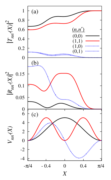
Figure 4: (Color online) Well and $\delta$-barrier. Barrier strength is $E_{\delta}=1$. With incident beam kinetic energy $E=4$, the only open channels are those labeled by $0$ or $1$. The transmission and reflection probabilities, $|T_{nn^{\prime}}(X)|^{2}$ and $|R{}_{nn^{\prime}}(X)|^{2}$, and the folded potentials $V_{nn^{\prime}}(X)$ are shown in panels (a), (b) and (c) for the open channels. $X$ is expressed in units of $\lambda$.

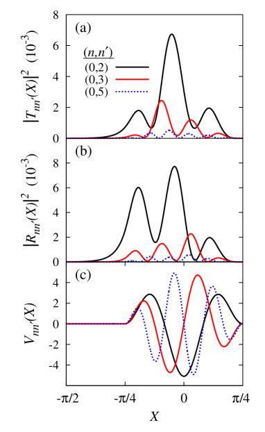
Figure 5: (Color online) Well and $\delta$-barrier. This graph refers to the same projectile as described in Fig. 4, with $E=4$. The reflection and transmission cross sections, $|R_{nn^{\prime}}(X)|^{2}$ and $|T_{nn^{\prime}}(X)|^{2}$, the folded potentials $V{}_{nn^{\prime}}(X)$ are shown for the out-going channel, $n=0$, for a projectile in three virtual incoming channels $n^{\prime}=2,\>3,\>5$. $X$ is expressed in units of $\lambda$.

In each of these figures, the lower panel (c) shows folded potentials, as follow from Eqs. (41) and (22). Thanks to the simplicity of $\delta$-barrier; the folded potentials have obvious forms showing the structures of the wave functions for the intrinsic square well confinement. Naturally, $V_{nn^{\prime}}(X)=0$ outside the well, or, in other words, if $|{x}|\geq\pi/2$ (that is, $|X|\geq\pi/4$) where $x$ (as well as $X$) is expressed in units of $\lambda$.

As explained through Fig. 3, the dynamic transmission and reflection amplitudes, $T(X)$ and $R(X)$, in the VPM correspond to the potential truncated from the left of $X$. Therefore, both transmission and reflection probabilities $|T_{nn^{\prime}}(X)|^{2}$ and $|R_{nn^{\prime}}(X)|^{2}$ shown in panels (a) and (b), respectively, are evolved from right to left following Eqs. (34) and (37). For both Figs. 4 and 5 we utilize the final state normalization (37) of $T(X)$ instead of $\overline{T}(X)$, due to the convenience in application and interpretation of $T$ as the transmission amplitude.

Figure 4 shows the dynamics in the open channels. Since the intrinsic potential is of a finite width, the final values of the reflection and transmission coefficients are reached at $X=-\pi/4$ which means inclusion of the full potential. And therefore, the values of $|R_{nn^{\prime}}(X)|^{2}$ and $|T_{nn^{\prime}}(X)|^{2}$ at $X=\pm\pi/4$ are the asymptotic values thereof, commensurate with (34) and (37). The probability is conserved at all values of $X$:

$$\sum_{n\in\mathrm{open}}|T_{nn^{\prime}}(X)|^{2}+|R_{nn^{\prime}}(X)|^{2}=1,$$

and $R_{nn^{\prime}}(X)=R_{n^{\prime}n}(X)$ due to time reversal symmetry. However, $T_{nn^{\prime}}(X)\neq T_{n^{\prime}n}(X)$ due to the asymmetry in the truncated potential. Symmetry is recovered in the final $T$ since the full symmetric potential is covered at $X=-\pi/4$, where $|T_{nn^{\prime}}|^{2}=|T_{n^{\prime}n}|^{2}$, as seen in Fig. 4(a).

A different picture emerges with the virtual channels. The linearity and independence of initial conditions, discussed earlier, is important since it makes the normalization of virtual channels irrelevant for the S-matrix and other asymptotic reaction observables. Having said that, one can assume that $\overline{T}_{nn^{\prime}}(-\infty)=0$ if the initial channel $n^{\prime}$ is closed (Eq. (38)), and thus $\overline{T}_{nn^{\prime}}(X)=0$ for any $X$ due to linearity (33). However, an incident beam in some open channel $n^{\prime}$ generates virtual excitations $n$ that exist outside the potential. Therefore, $\overline{T}{}_{nn^{\prime}}(X)$ is an exponentially decaying non-zero function beyond the range of the potential when initial channel $n^{\prime}$ is open but the final channel $n$ is closed.

A totally different situation arises with the final state normalization (37), i.e., with $T_{nn^{\prime}}(\infty)=0$ if $n$ corresponds to a closed channel. Thus assuming that all virtual channels are normalized to zero to the right of the barrier generates disturbances of virtual channels in front of the potential barrier, so that $T_{nn^{\prime}}(X)$ is not zero there when $n^{\prime}$ is closed. This is seen in Fig. 5 where such quantities $T_{nn^{\prime}}(X)$ (or, their norms) decay exponentially to the left of the barrier, but are not zero at $X=-\pi/4$.

The interpretation of $R_{nn^{\prime}}(X)$ is quite different. It sets relations between the different components (phase shifts) of the wave function, and is non-zero for all real and virtual initial and final channels. Nevertheless, the behavior is similar (see Fig. 5).

V.1.2 Results

Let us now discuss some final results for the scattering and tunneling of the deuteron-like system. Here we continue to consider the infinite square well (“well”) and the harmonic oscillator (“HO”) models (see Sec. III.1.1 and III.1.2), that do not allow for breakup. A model with a continuum of intrinsic states, which allows for breakup, is described in Sec. VII.

Figures 6 and 7 for the “well,” and Figs. 8 and 9 for the “HO,” depict the probabilities $|T_{n}|^{2}$ of transmission and $|R{}_{n}|^{2}$of reflection, respectively, in the first few lowest channels as functions of incident beam kinetic energy $E$. Each figure contains vertical grid lines indicating the locations of channel thresholds. In the case of the "well," new channels open up at kinetic energies $E=n^{2}-1$ where $n$ is a positive integer; for the "HO," these occur at integral multiples of $\hbar\omega$. In each case the incident beam is in the ground state channel, thus the corresponding subscript is suppressed, and $n$ refers to the final channel. The strength of the $\delta$-barrier is set, via Eq. (42), to $E_{\delta}=1$. The redistribution of probabilities at the threshold energies, required by unitarity, leads to cusps in the cross sections Landau and Lifshitz (1981); Baz et al. (1971). These discontinuities are common in all the figures for both the models.

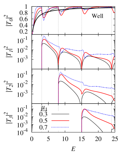
Figure 6: (Color online) Well and $\delta$-barrier. Barrier strength $E_{\delta}=1$. Probabilities of transmission to different final channels $n=0,\,1,\,2\>\textrm{and}\>3$ are shown as functions of incident beam kinetic energy $E$. The incident beam is in the ground state channel. The different curves on each panel correspond to different values of the mass-ratio $\mu_{1}$, as labeled. The non-composite limit is shown in the top panel with the thick solid line.

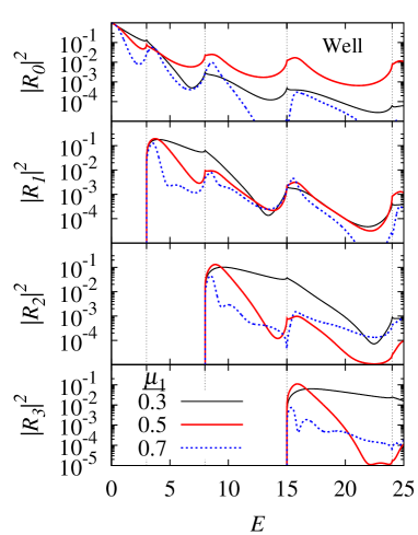
Figure 7: (Color online) Well and $\delta$-barrier. Same as Fig. 6, showing reflection probabilities.

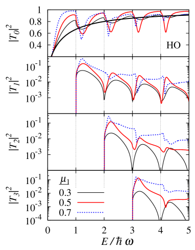
Figure 8: (Color online) HO and $\delta$-barrier. Barrier strength $E_{\delta}=1=0.5\>\hbar\omega$. Probabilities of transmission to different final channels $n=0,\,1,\,2\>\textrm{and}\>3$ are shown as functions of incident beam kinetic energy $E$. The incident beam is in the ground state channel. The different curves on each panel correspond to different values of the mass-ratio $\mu_{1}$, as labeled. The non-composite limit is shown in the top panel with the thick solid line.

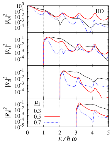
Figure 9: (Color online) HO and $\delta$-barrier. Same as Fig. 8, showing reflection probabilities.

All figures contain three curves with $\mu_{1}=0.3,\>0.5\>\mathrm{and}\>0.7$, and thus illustrates the mass-ratio dependence. In addition to that are shown the ground state to ground state transmission probabilities in the top panels of Figs. 6 and 8 in the non-composite limit $\mu_{1}\to 0$ where an analytic answer follows from Eq. (43). Indeed, when the non-interacting particle-1 is very light compared to the interacting particle-$2$, i.e., when $\mu_{1}\rightarrow 0$, then particle-$2$ carries almost all the momentum, and the presence of particle-$1$ hardly matters. In this limit the behavior of the projectile approaches that of a single non-composite particle.

The development of the resonant behavior, as $\mu_{1}$ increases, is easy to follow in these plots. For larger values of $\mu_{1}$ the curves exhibit prominent peaks and dips that are not associated with cusps at thresholds. Classically this can be viewed as a process in which the light interacting particle is stopped by the potential, while the larger mass $\mu_{1}$ keeps moving forward without any impediment, until most of its kinetic energy is transferred into potential energy of the intrinsic interaction, and then it either turns back or pulls the smaller interacting mass through the barrier. Hence, the larger the non-interacting particle’s mass, the more complex and chaotic the process.

It is intuitive to suggest that the highly virtual channels have little or no effect on observables at low-energies. It is proved otherwise in our studies. In Figs. 10 and 11 we focus on the low energy region, below the first threshold, for the "well" and the "HO" models, respectively. Here we use the same parameters as in Figs. 6-9, and present our results for the non-composite limit $\mu_{1}=0$ as well as for projectiles with $\mu_{1}=0.3,$ 0.5, and 0.7. Along with the transmission probability, we show results for the two phase shifts (9) that are defined up to the first threshold (shown by the vertical grid line). We conclude that the compositeness, and the composition of the projectile given by the mass-ratio of the components, are consequential factors that determine the observables. In these models, as well as in the ones with breakup (discussed in Sec. VII), we find a systematic enhancement of tunneling probability, with increasing mass of the non-interacting component, in a broad region of energy near the first threshold. This enhancement was earlier discussed in Ref. Ahsan and Volya (2007). This is supported by a recent experimental at GANIL by Lemasson and others Lemasson et al. (2009) that shows enhancement in tunneling of heavy He isotopes, where additional spectator-neutrons contribute to the mass of the non-interacting component, while the alpha core interacts with the Coulomb barrier.

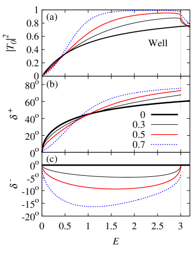
Figure 10: (Color online) Well and $\delta$-barrier. The system is same as that in Fig. 6, showing transmission probability $|T_{0}|^{2}$ for energies below the first threshold in panel panel (a), and phase shifts $\delta^{\pm}$ for the same energy region in panels (b) and (c).

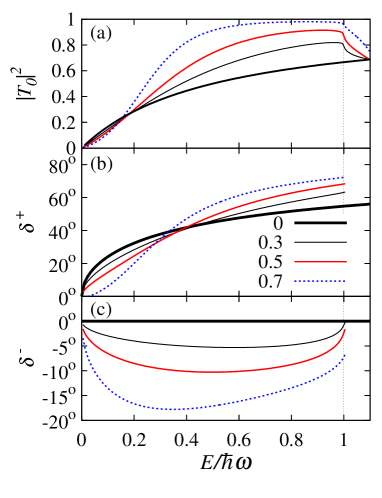
Figure 11: (Color online) HO and $\delta$-barrier. The system is same as that in Fig. 8, showing transmission probability $|T_{0}|^{2}$ for energies below the first threshold in panel panel (a), and phase shifts $\delta^{\pm}$ for the same energy region in panels (b) and (c).

V.1.3 An attractive $\delta$-well

In addition to the $\delta$-barrier discussed so far, we explored scattering that involves an attractive $\delta$-well. We stress again that for a non-composite projectile the sign of the interaction does not effect the observed reflection and transmission probabilities (see Eq. (44)). This is not true for a composite projectile. This topic has been extensively explored in the literature and is often referred to as the Barkas Effect. In Ref. Volya and Esbensen (2002), one can find more references that are relevant, and a model that is similar in spirit and discusses the Coulomb excitation of a harmonic oscillator.

Our results for the transmission probability in a scattering that involves a $\delta$-well are shown in Fig. 12. We present results for the case of a harmonic-oscillator confinement only; the results for the square well are similar. In all cases, even at relatively small masses of the non-interacting component, the scattering process is highly resonant. The interacting particle-2 and the barrier form a bound state at an energy $-\mu_{2}E_{\delta}$, which is only a virtual binding in the three-body problem. However, the system in an excited state $n$ with intrinsic energy $\varepsilon_{n}$ can be temporarily bound as a whole, thus leading to a resonance at $E_{T}=\varepsilon_{n}-\mu_{2}E_{\delta}$. We find that this crude interpretation unravels some of the complex resonant patterns seen in Fig. 12. The resonances indeed periodically follow the channel thresholds, and they are close to the thresholds for small $E_{\delta}=1$ (upper panel) and are further away for the larger $E_{\delta}=5$ (lower panel).

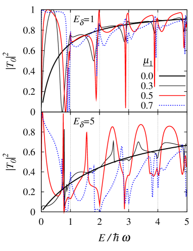
Figure 12: (Color online) Well and attractive $\delta$-well. The probability of transmission from ground state to ground state is shown as a function of incident kinetic energy. The upper and lower panels correspond to the barrier-strengths $E_{\delta}=1$ and 5 (i.e., 0.5$\,\hbar\omega$ and 2.5$\,\hbar\omega$), respectively. In both cases three different mass-ratios $\mu_{1}=0.3,$ 0.5, and 0.7 are considered, along with the analytic limit of a non-composite projectile (labeled by $\mu_{1}=0$).

V.2 An infinite wall

In this section we would like to return to the wall problem which, as already shown in Sec. III, is an extraordinarily illustrative example. This model emerges in the limit of a very strong $\delta$-potential (Sec. V.1), i.e., with $A\rightarrow 0$.

We study the convergence of the VPM method separately in Sec. VI; nevertheless, here we present Fig. 13 which, in contrast to Fig. 2, shows that the VPM method is not prone to the convergence issues. Even for the large mass-ratio $m_{1}/m_{2}=5$ the VPM produces a perfectly smooth curve that converges to a final $\delta=-77{}^{o}$, which is not the case with the Projection Method.

Figure 13: (Color online) HO and wall. This figure refers to the scattering problem described in Fig. 2, where the system of two particles bound by "HO" confinement collides with an infinite wall. The incident kinetic energy is $E=1=0.5\,\hbar\omega$, and the mass-ratio is $m_{1}/m_{2}=5$. The phase $\delta$, as calculated using the VPM, is plotted in the solid line against the number of included channels $N$. The horizontal grid line indicates the final value of the phase shift to which it is found to converge smoothly with increasing $N$. The dashed curve shows results obtained through the Projection Method, which is unstable.

Figures 14 and 15 show the reflection probabilities of a composite projectile in the ground state channel scattered from a wall. They are similar to the previous results for scattering that involves a $\delta$-barrier (see Sec. V.1.2); cusps at thresholds and some resonant behavior are among the typical features.

Figure 14: Well and wall. This is the same as Fig. 7, but for a “wall,” not for a $\delta$-barrier, and only for the case of equal masses, $m_{1}=m_{2}$ (i.e., $\mu_{1}=0.5$).

Figure 15: HO and wall. This is the same as Fig. 9, but for a “wall,” not for a $\delta$-barrier, and only for the case of equal masses, $m_{1}=m_{2}$ (i.e., $\mu_{1}=0.5$).

Scattering below the first threshold is characterized by a single phase shift $\delta$, which is plotted in Fig. 16 as a function of incident beam kinetic energy, in the case of the harmonic oscillator. The different curves correspond to different mass-ratios.

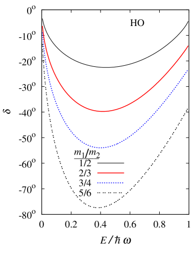
Figure 16: (Color online) HO and wall. Phase shift as a function of incident beam kinetic energy. The curves are labeled with different values of the mass-ratio $m_{1}/m_{2}$.

The limit of very low energies is particularly interesting. The formal effective range expansion Levy and Keller (1963); Dashen (1963); Calogero (1967); Babikov (1968), in the context of the VPM, has been applied extensively to problems of nucleon, molecular, and atomic scattering. As $K\rightarrow 0$, the $S$-matrix, $S=e^{2i\delta}$, is characterized by a phase $\delta=-Ka$ where $a$ is the scattering length. This length $a$ depends only on the mass-ratio $m_{1}/m_{2}$ and represents the distance of the turning point from the reflecting wall. A scattering length $a>0$ implies that the system is reflected at a distance $a$ prior to reaching the wall. Figure 17 shows $a$ in units of $\lambda$, as a function of $\mu_{1}$. The limit $\mu_{1}\to 0$ corresponds to a non-composite case where the scattering length is zero. It is interesting to note that, while the intrinsic wave function of an infinite square well confinement has a finite width $\sim\pi\lambda$, the scattering length can easily exceed this range. Thus, a classically impossible situation occurs in which a finite-size system reflects from a wall before it actually approaches it within the contact distance. In the limit of $\mu_{1}\rightarrow$1 the scattering length ${a}$ diverges. This is a strong divergence since it is relative to a divergent scale, $\lambda\rightarrow\infty$ for any given energy because of the vanishing reduced mass. It is worth pointing out that the divergence of the scattering length due to intrinsic degrees of freedom coupling to the reaction dynamics is known as Feshbach Resonance.

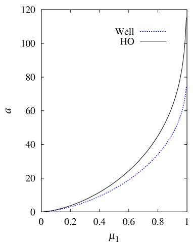
Figure 17: (Color online) Well/HO and wall. For the “deuteron and Coulomb wall” model, the scattering length $a$ (in units of intrinsic length $\lambda$) is shown as a function of the mass-ratio $\mu_{1}=m_{1}/M$ for two different systems: those bound by the “well” and by the “HO” confinements.

For both square well and oscillator models one can examine the analytic results for ${a}$ by considering a few virtual channels within the Projection Method. It becomes immediately clear that such an expansion is convergent only in the limit of $\mu_{1}\rightarrow 0$. In this limit we obtain ${a/\lambda}\approx 0.56\,\mu_{1}^{3/2}$ for the square well bound system, and ${a/\lambda}=\mu_{1}^{3/2}$ for the oscillator-bound system.

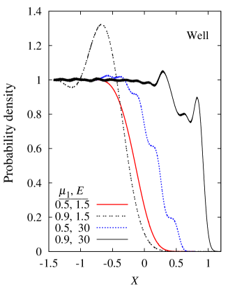
Figure 18: (Color online) Well and wall. Probability densities as functions of location, for scattering of a square-well-bound system off an infinite wall at $X=0$.

Figure 18 shows the square of the amplitude of the wave function, $\underset{n}{\Sigma}|\overline{T}_{nn^{\prime}}(X)|^{2}$, for a projectile in the incoming channel $n^{\prime}=0$. This is interpreted as the density of probability for the center of mass of the projectile to be at a location $X$ when it is reflected from an infinite wall. The four curves show a few of the most representative situations; incident beam kinetic energies as low as $E=1.5$ and as high as 30, and two different mass-ratios $\mu_{1}=0.5$ and 0.9. All probabilities eventually die to zero beyond the wall located at $X=0$. The first two curves represent cases where the energy of the projectile, $E=1.5$, is halfway between the energies of the ground state and the first excited state. Hence only one open channel is present. For mass-ratio $\mu_{1}=0.5$ the behavior is plain. However, when the non-interacting particle contains 90% of the total mass there is a peak of probability density in front of the wall. This is consistent with the enhanced scattering length (see Fig. 17) and with its interpretation that this probability peak corresponds to a turning point where the system is stopped prior to reaching the wall. At higher beam energies the center of mass penetrates considerably through the wall (region $X>0).$ As expected, this penetration is deeper for a more massive non-interacting component; the peaks in the density inside the wall can also be attributed to the non-interacting particle being stopped via energy transfer to intrinsic excitations.

VI Role of virtual channels and convergence

While problems similar to those presented here have been extensively discussed in recent literature, for example Refs. Shegelski et al. (2008b, a); Razavy (2003); Saito and Kayanuma (1994); Hnybida and Shegelski (2008); Goodvin and Shegelski (2005); Bacca and Feldmeier (2006), little attention has been paid to virtual channels. In fact, most of these works discuss tunneling of a diatomic molecule where both the atoms interact with the potential. In that case, virtual excitations are relatively less likely to take place, and hence the folded potential within open channels already provides a relatively good description of the process. Our selection of models on the other hand, where only one particle interacts with the scatterer, is dynamically different. It is the virtual channels that shape the non-interacting particle’s movement. Therefore, compared to the models discussed by other authors cited above, our models are in general more sensitive to virtual channels. In the most extreme case of reflection from an infinite wall, no meaningful description is possible at all without reference to the virtual channels. The folded potential for the ground state, depicted in Fig. 4(c) with the solid black line, has a single hump, and therefore does not lead to any resonant behavior in reactions at low energies, when only one channel is open. Hence it can be concluded that, the resonance-like increases or decreases in the transmission and reflection probabilities shown, for example, in Figs. 8 and 9, at low energies and especially when the non-interaction particle is heavy, are exclusively due to virtual channels.

A successful extension of the VPM so as to include virtual channels in the formalism, and the study of their role that we discuss in this section, are among the main achievements of this work.

The importance both of compositeness and of virtual channels is illustrated in Fig. 19, where we consider an oscillator scattering from a $\delta$-barrier. The curves in three different styles and colors correspond to results from three different calculations: the solid red line represents the exact solution, i.e., the solution of scattering of a composite projectile obtained through a calculation that includes the virtual channels as well as the open channels; the dotted blue line represents scattering of a composite projectile solved through a folded potential but ignoring any virtual channel whatsoever; the solid black line represents scattering of a non-composite projectile of the same mass as that of the composite projectile. For the region of energies shown in these graphs, there is only one open channel; thus the asymptotic behavior of the wave function is fully determined by the two phase shifts $\delta^{\pm}$ which are shown in panels (b) and (c) as functions of incident beam kinetic energy. All three curves are different, indicating that neither non-compositeness nor treatment of open channels only can substitute for a full solution. To emphasize this, we show in panel (a) transmission probability, an observable quantity, as a function of energy; for most of the energy region shown, the actual transmission probability appears to be higher than that of an equally massive non-composite particle.

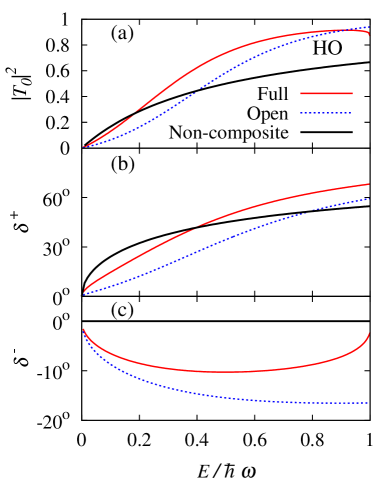
Figure 19: (Color online) HO and $\delta$-barrier. A two-body system with $m_{1}=m_{2}$, bound by an oscillator confinement, is scattered by an external delta potential with $E_{\delta}=1$. Panels (a), (b), and (c) correspond to transmission probability, and two symmetric and antisymmetric phase shifts, respectively. Three curves shown compare full solution (labeled “full”) with the approximate treatment that includes only the open channels (“open”), and with results for non-composite projectile (“non-composite”). We conclude that ignoring the composite nature of the system or neglecting the virtual channels results in neither the phase shifts nor the transmission probability correctly.

While the virtual channels cannot in general be ignored, the contribution of the highly excited states is expected to diminish. Practical applications require some truncation in the channel space, too. In Fig. 20(a) we demonstrate the rate of convergence of the transmission probability $P_{T}=|T_{0}|^{2}$ by plotting it as a function of the number of included channels $N$. The curve is visually indistinguishable from the hyperbola

$$P_{T}(N)=P_{T}-\frac{N_{s}}{N},$$ (45)

showing that the deviation of the probability $P_{T}(N)$ from its limiting value $P_{T}$ is inversely proportional to $N$. That is, $N_{s}$ is the rate of convergence. The lower plot, Fig. 20(b), shows agreement with Eq. (45) by comparing $\left[P_{T}-P_{T}(N)\right]N$ with a constant $N_{s}$. These results are for the square well bound system with $|K_{N}|\sim N$. With more precise consideration it is found that in general, the amplitudes converge as $\sim 1/|K_{N}|.$ Figure 21 demonstrates an excellent agreement with this rule using two different systems reflecting from an infinite wall.

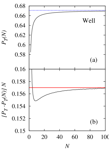
Figure 20: (Color online) Well and $\delta$-barrier. Convergence of the transmission probability $P_{T}=|T_{0}|^{2}$ to its limiting value, as a function of $N$. The masses are equal, $m_{1}=m{}_{2}$, and the kinetic energy is $E=4$, so that only the first two channels are open. The strength of the $\delta$-barrier is $E_{\delta}=1$. Plot (a) shows the actual behavior of the transmission probability $P_{T}(N)$ with $N$, and its asymptotic value $P_{T}=0.6708$ shown by the grid-line. In order to show agreement with Eq. (45), the value $N\left[P_{T}-P_{T}(N)\right]$ is shown in plot (b). This quantity is well described by a constant $N_{s}=0.157,$ shown with the red horizontal line.

Figure 21: Well/HO and wall. Convergence of the phase shift. The log-log scale acts to accentuate a good agreement with the $\sim 1/|K_{N}|$ convergence rule. The dashed straight lines represent these rules. For the square well intrinsic potential, $K_{N}\sim N$ and $\delta(N)\simeq\delta-N_{s}/N$ with $\delta=-23.05^{\circ}$ and $N_{s}=11.3.$ For the harmonic oscillator $K_{N}\sim\sqrt{N}$, so $\delta(N)\simeq\delta-\sqrt{N_{s}/N}$ with $\delta=-22.98^{\circ}$ and $N_{s}=53.4$. For both cases the incident beam energy is halfway between those of the ground state and the first excited state.

This power-law convergence is slow in contrast to an exponential convergence usually encountered for eigenvalues and other structural observables as functions of truncation Horoi et al. (1999). Here we repeat our recent conjecture Ahsan and Volya (2010) that this is an inherent property of reaction physics, where the kinetic energy operator plays a major role in the Hamiltonian. The mentioned operator discretized in coordinate space corresponds to a tri-diagonal matrix that meets a set of criteria for the power-law convergence Horoi et al. (1999).

In the course of our work we have vigorously tested the $\sim 1/|K_{N}|$ convergence rule. While the rate of convergence, $N_{s}$, depends strongly on the type of the system, we found no exception from the power-law convergence.

VII Intrinsic potential with a continuum; breakup

We would like to conclude our exploration with a somewhat more realistic situation where the intrinsic potential allows for a breakup. We therefore consider a confining potential $v(x)$ that has both bound state(s) and a continuum. In our discussion below we study a particular confinement, namely, a finite square well ("finite well"):

$$v(x)=\left\{\begin{array}[]{cc}0&\text{when}\,\,|x|>\lambda\\ -v&\text{otherwise}\end{array}\right.\,.$$ (46)

This allows one to capture the generic features of the problem, while still having a small number of parameters and retaining the ability to have analytic solutions (5) for the intrinsic Hamiltonian. Realistic applications to three-dimensional problems with other potentials are outside the scope of this work.

In what follows we again select the units of length $\lambda$ to represent the width of the intrinsic potential as defined in Eq. (46). The bound state energies for the finite square well potential are given by the transcendental equation

$$\tan\sqrt{\varepsilon+v}=\pm\left(\frac{-\varepsilon}{v+\varepsilon}\right)^{\pm 1/2},$$ (47)

where we remind the reader that $v$ and $\varepsilon$ are expressed in units of $\epsilon$ [see (17)]. The $\pm$ sign corresponds to the intrinsic parity ${\cal P}=\pm 1$ of the state of interest. In addition to these bound states there is a continuum of states with positive energies above the well.

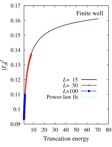
Figure 22: (Color online) Finite well and $\delta$-barrier. Convergence of the transmission probability to its final value with truncation energy (in units of $\epsilon$) of virtual excitations. The well-depth is $v=1$ and the incident kinetic energy is $E=0.2$. Therefore, only the elastic channel is open. The figure contains four different curves, three of which are labeled with the widths of the quantization box, $L=15,\,50,\>{\rm\text{{and}}}\>100$ that were used. These curves agree well with the power-law convergence discussed in the previous section, the fit for which is shown with the last curve (green, dashed). The final value for transmission probability is 0.174.

To model such a situation mathematically we discretize the spectrum using a quantization-box of width $2L$, and hence the intrinsic wave functions $\psi_{n}(x)$ are subject to a boundary condition $\psi_{n}(\pm L)=0$. The choice of a large enough $L$ can yield a spectrum that represents the continuum obtained without the box. The large box allows for any finite potentials $v(x)$ to be considered.

In order to examine the appropriateness of the approach and to address the potential concerns arising from the presence of the continuum and its truncation, we show in Fig. 22 the calculated transmission probability for such a system incident on a $\delta$-barrier. A depth of $v=1$ has been chosen for this example, thus there being a single bound state at energy $\varepsilon_{0}=-0.454$, as follows from Eq. (47), with the RMS size $1.17$ of the wave function. The incident kinetic energy of the center-of-mass motion is assumed to be $E=0.2$, which means that only the elastic channel is open. Though there is not enough beam energy for a breakup, the virtual channels are still important. In Fig. 22 we explore different box-widths, $L=15,\,50,$ and $100$ (in units of $\lambda$), which shows that the results are independent of $L$, if it is large enough. (Note that with a large box-width the density of states in the continuum is high and therefore it is difficult to include high-energy channels.) Even for the smallest box $L=15$ the energy of the ground state differs from the exact answer only by less than 0.05%. The breakup threshold is at $0.495$, which is slightly different from $-\varepsilon_{0}$ mainly because the first excited state (continuum threshold) in the box does not exactly coincide with zero energy. These differences are minor and orders of magnitude smaller for $L=100.$

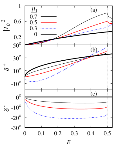
Figure 23: (Color online) Finite well and $\delta$-barrier. Transmission probability and phase shifts for the scattering of a two-particle system with intrinsic potential that is finite and allows for breakup. The potential is modeled by a square well of unit width and depth $v=1.$ We concentrate on the region below the breakup threshold of kinetic energy at $0.495$ shown with the vertical grid-line. Four curves correspond to four different mass-ratios $\mu_{1}=0.3,\;0.5,\;\mathrm{and}\;0.7$ and the non composite limit of $0$ for which Eq. (43) is plotted. The $\delta$-barrier strength is assumed to be $E_{\delta}=1$. The upper panel shows transmission probability; the curve is continued above the breakup threshold to show the cusp at the threshold. The two lower panels, similar to those in Figs. 11 and 10, show the phase shifts $\delta^{+}$ and $\delta^{-}$ as defined in Eq. 9. Note that their meanings as phase shifts of the S-matrix is true only below the breakup threshold; above the breakup these are arguments of the corresponding reflection and transmission amplitudes.

Now that the appropriateness and validity of the approach is established, we present the transmission probability and both symmetric and antisymmetric phase shifts $\delta^{\pm}$ as functions of incident kinetic energy in Fig. 23. This figure concentrates on the energy region below the breakup threshold. This situation is important, since it is commonly encountered in practice. As it is clear from the graphs, the composite nature of the system and the virtual continuum are playing a crucial role in shaping the reaction process. We find that at very low energies transmission is inhibited for a composite particle. At higher energies close to the breakup threshold, transmission rate is always enhanced. Moreover, this rate increases for an increasingly heavy non-interacting particle. The role of the virtual channels appears to be universal for all models that we investigated [see also Figs. 6 and 8], where $|T_{0}|^{2}$ increases sharply near the first threshold. The experiment in GANIL, as cited at the end of Sec. V.1.2, proves tunneling enhancement for systems with breakup also.

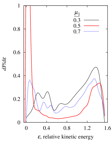
Figure 24: (Color online) Finite well and $\delta$-barrier. Probability to break up into a level $\varepsilon$ in the continuum is plotted as a function of $\varepsilon$. The intrinsic potential is modeled by a square well of unit width and depth $v=1$, as described in the text. The kinetic energy of the incident wave is $E=2$. The system interacts with a $\delta$-barrier of strength $E_{\delta}=1$, and then either scatters elastically, or breaks up into its constituents with relative energy $\varepsilon$. The three curves correspond to three different mass-ratios $\mu_{1}=0.3,\;0.5,\;\mathrm{and}\;0.7$. The corresponding probabilities for elastic scattering are $0.64$, $0.60$, and $0.69$ respectively, which complement the breakup probabilities shown here.

It is interesting to review the distribution of probability of breakup into the continuum, when energetically possible. In the continuum we can still separate the center-of-mass and the relative kinetic energies. The relative kinetic energy is now given by the discretized states in the box. Fig. 24 shows the normalized probability distribution for breakup with different relative energies. The initial beam in this case corresponds to a projectile in the ground state with kinetic energy of $E=2$. Thus, the total kinetic energy of fragments after the breakup is ${E}+\varepsilon_{0}-\varepsilon_{1}\approx{E}+\varepsilon_{0}=1.55$ which is viewed as a sum of two parts: the center-of-mass kinetic energy $\hbar^{2}K^{2}/(2M)$ and the relative kinetic energy $\varepsilon$. As seen from the plot, it is most likely to have the two fragments moving together with very little relative energy (corresponding to the peaks on the left side of the plot), or, inversely, moving apart in opposite directions with most of the energy concentrated in the relative motion (corresponding to the peaks on the right side).

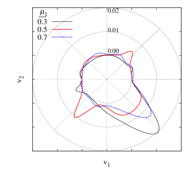
Figure 25: (Color online) Finite well and $\delta$-barrier. The system and scattering conditions are the same as in Fig. 24. The system interacts with the $\delta$-barrier, and then either scatters elastically, or breaks up into its constituents with momenta $\mathrm{v}{}_{1}$ and $\mathrm{v}_{2}$. Break-up probability, as a function of velocities $\mathrm{v}_{1}$ and $\mathrm{v}{}_{2}$, is plotted as a contour graph. Due to Eq. (48) the points representing the possible velocity values lie on an ellipse in the $\mathrm{(v}{}_{1},\,\mathrm{v}{}_{2})$ plane and are parametrized by a single angle. The contour plot shows the probability of breakup (radial coordinate) as a function of this angle.

The choice of quantities plotted in Fig. 24 reflect our method, but is not very closely related to a potential experiment, where the momenta or velocities of both particles could be measured. Therefore in Fig. 25 we show the distribution of probability to observe a certain combination of the particle-velocities $\mathrm{v}_{1}$ and $\mathrm{v}_{2}$. Since the total kinetic energy after breakup is fixed,

$$\frac{1}{2}\left(m_{1}\mathrm{v}_{1}^{2}+m_{2}\mathrm{v}_{2}^{2}\right)=E+\varepsilon_{0},$$ (48)

it is sufficient to use a single angle to parametrize the position on the ellipse formed in the velocity $(\mathrm{v}_{1},\,\mathrm{v}_{2})$ plane. In Fig. 25 we show the probability as a function of angle using a contour plot. Both Figures 24 and 25 have been smoothed, but preserve the general shapes which we believe to be good representations of the physics. Some of the features seen in Fig. 24 become more transparent in Fig. 25. For all mass-ratios we see that the probability peaks at about $-45^{\circ}$ which corresponds to non-interacting particle-1 moving forward and interacting particle-2 being reflected back with velocities nearly equal in magnitude and opposite in direction. For equal masses the peak at low relative kinetic energies in Fig. 24 appears as two peaks in Fig. 25 at about $45^{\circ}$ and $-135^{\circ}$. In both cases the particles move with similar velocities, forward for $45^{\circ}$ and backward for $-135^{\circ}.$ The observed picture appears to be quite intuitive.

VIII Summary and conclusions

In this work we revisit some of the most intricate questions of reaction physics involving composite objects. The research presented here was inspired by highly unpredictable behavior of reaction observables including resonances and cusp-discontinuities, a very broad spectrum of scales involved, and, at the same time, the utmost importance of these processes in nuclear physics and other fields.

The topic of reactions involving composite objects is widely investigated, and benefits from many advanced methods and techniques. Our work got its thrust from a simple and well-defined problem of a deuteron-like system interacting in one dimension with an infinite Coulomb wall. A number of methods tried, in the past, for this problem have failed under certain circumstances, namely, where approximations or simplifications commonly used were not appropriate for this particular problem, or where the method did not produce convergent results, or where there were difficulties with numerical errors. Due to this delicate nature of the problem, we find exact solutions to all the examples considered in this work. This allows us to obtain comprehensive answers, and to be able to carry out comparisons with other methods and solutions.

This goal requires us to have a precisely-defined Hamiltonian with as few parameters as possible, and conditions that perhaps are more critical to reaction-structure interplay than those typically encountered in nature. In this presentation we restrict our discussion to models. Nevertheless, our methods have broad applicability; most examples can be modified easily to represent realistic situations, and we continuously suggest cases in nature that are similar to what we discuss. We study, through this work, a two-particle system interacting in a one-dimensional scattering with a target that poses a $\delta$-potential or an infinite wall potential. It is always assumed that only one of the two components interacts with the target. The study includes models that do allow the projectile to breakup, and models that do not. The dominant and non-perturbative role of the virtual channels that extend far in excitation energy is the main common theme of all the examples discussed here.

We start by revisiting the "deuteron and Coulomb-wall" model which has been discussed for almost a decade with little outcome Moro et al. (2000); Sakharuk ; Ahsan and Volya (2007). Unfortunately, this problem is commonly dismissed either at the first glance when it seems uninteresting, or after some investigation when it seems unphysical, ill-defined, or unsolvable. We, on the other hand, find this model remarkable in its ability to demonstrate, in an extremely transparent manner, the dynamics driven by the virtual excitations.

We review, and carefully apply, the technique of projecting the reaction dynamics onto an intrinsic space and show that while satisfactory results are obtained in some limits, this formally exact approach does not yield convergent solutions in general. This is an important finding because this “Projection Method” is a prototype of several commonly used approaches in many-body problems that involve both structure and reactions Okolowicz et al. (2003); Volya and Zelevinsky (2006).

As our main workhorse we utilize the Variable Phase Method (VPM) to address the coupled-channel problems of interest. While the method has been used by others before, we modify and extend it to treat highly remote virtual channels. We demonstrate that the VPM produces reliable and convergent results. We investigate the contributions from remote virtual excitations, study convergence with the truncation size, and find the power-law convergence, which is in contrast to the exponential convergence seen in many-body structure problems Horoi et al. (1999).

Within a given set of models, this work contains numerous examples, investigations and demonstrations. Cusps and discontinuities appear in observables as manifestations of conservation of probability and redistribution of flux at the thresholds. Intrinsic structure gives rise to resonance-like behavior in tunneling probabilities; our models and recent experimental evidences indicate a generic enhancement in transmission probabilities due to virtual channels or a virtual continuum, whichever is the case. We explore and discuss the role of virtual excitations at very low energies, showing that even in those cases the scattering length is sensitive to the projectile’s structure. Due to the intrinsic structure and its coupling to reaction dynamics, scattering length can become infinite, the phenomenon being known as Feshbach resonance. We demonstrate how the intrinsic structure violates charge symmetry, which is called the Barkas effect. The scattering of a non-composite projectile off a $\delta$-barrier is the same for attractive and repulsive interactions. But, in case of a composite projectile, the corresponding three-body problem for an attractive potential is quite different from that for a repulsive barrier, and reveals numerous resonances, some of which can be understood as bound states built upon individual intrinsic excitations involving two-body subsystems.

Scattering and breakup dynamics influenced by a virtual continuum are also investigated in this work. It is seen that the most probable breakups take place where either almost all the kinetic energy is relative, or almost all of it is in the center of mass.